A synthetic map of the north-west European Shelf sedimentary environment for applications in marine science - ESSD
←
→
Page content transcription
If your browser does not render page correctly, please read the page content below
Earth Syst. Sci. Data, 10, 109–130, 2018
https://doi.org/10.5194/essd-10-109-2018
© Author(s) 2018. This work is distributed under
the Creative Commons Attribution 4.0 License.

                    A synthetic map of the north-west European
                        Shelf sedimentary environment for
                          applications in marine science
                    Robert J. Wilson, Douglas C. Speirs, Alessandro Sabatino, and Michael R. Heath
                             812 Livingstone Tower, Department of Mathematics and Statistics,
                            University of Strathclyde, 26 Richmond Street, Glasgow G1 1XH, UK
                              Correspondence: Robert J. Wilson (robert.wilson@strath.ac.uk)

                                   Received: 7 August 2017 – Discussion started: 18 August 2017
                      Revised: 20 November 2017 – Accepted: 29 November 2017 – Published: 23 January 2018

       Abstract. Seabed sediment mapping is important for a wide range of marine policy, planning and scientific
       issues, and there has been considerable national and international investment around the world in the collation
       and synthesis of sediment datasets. However, in Europe at least, much of this effort has been directed towards
       seabed classification and mapping of discrete habitats. Scientific users often have to resort to reverse engineering
       these classifications to recover continuous variables, such as mud content and median grain size, that are required
       for many ecological and biophysical studies. Here we present a new set of 0.125◦ by 0.125◦ resolution synthetic
       maps of continuous properties of the north-west European sedimentary environment, extending from the Bay of
       Biscay to the northern limits of the North Sea and the Faroe Islands. The maps are a blend of gridded survey
       data, statistically modelled values based on distributions of bed shear stress due to tidal currents and waves,
       and bathymetric properties. Recent work has shown that statistical models can predict sediment composition
       in British waters and the North Sea with high accuracy, and here we extend this to the entire shelf and to the
       mapping of other key seabed parameters. The maps include percentage compositions of mud, sand and gravel;
       porosity and permeability; median grain size of the whole sediment and of the sand and the gravel fractions;
       carbon and nitrogen content of sediments; percentage of seabed area covered by rock; mean and maximum
       depth-averaged tidal velocity and wave orbital velocity at the seabed; and mean monthly natural disturbance
       rates. A number of applications for these maps exist, including species distribution modelling and the more
       accurate representation of sea-floor biogeochemistry in ecosystem models. The data products are available from
       https://doi.org/10.15129/1e27b806-1eae-494d-83b5-a5f4792c46fc.

1   Introduction                                                   particularly those due to trawling (Diesing et al., 2013). The
                                                                   evolution of deltas is strongly influenced by sediment com-
Knowledge of the geographic variation in the sedimentary           position (Edmonds and Slingerland, 2009; Falcini and Jerol-
environment of the seabed is required for a wide variety of        mack, 2010). Mapping the sediment composition and physi-
marine planning and science tasks. Benthic species have dif-       cal environment of the seabed is therefore an integral part of
fering sediment requirements and seabed mapping can there-         understanding and managing benthic environments.
fore help identify ecologically distinct habitats (Robinson           The north-west European Shelf is one of the world’s sea
et al., 2011). Sediment type and wave and tidal regime are         regions most impacted by human activities (Halpern et al.,
important determinants of the rate of natural disturbance of       2014). These impacts are dominated by fishing, and it has
the seabed (Aldridge et al., 2015; Bricheno et al., 2015). The     been estimated that over 99 % of human impact on the seabed
composition of sediments also has a large influence on the         is from trawling (Foden et al., 2011). Existing maps of seabed
consequences of anthropogenic disturbance on the seabed,           sediments for this region have almost exclusively focused on

Published by Copernicus Publications.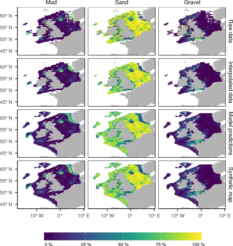
110                       R. J. Wilson et al.: Maps of the north-west European Continental Shelf sedimentary environment

the territorial waters of individual states (e.g. the British Ge-
ological Survey’s DigSBS250 product) or subregions (e.g.
the North Sea; Basford et al., 1993). Currently the EU Mesh
project is mapping benthic habitat classes across the north-
west European Shelf (Vasquez et al., 2015). However, no
existing research has mapped the continuous properties of
sediments across this region. Here we map key parameters
related to the sediment composition and the physical envi-
ronment of the seabed in an area extending from the Bay of
Biscay to the northern limits of the North Sea.
   This study was motivated by the need for openly available
datasets of the sedimentary environment for parameterizing
shelf sea ecosystem models (e.g. Baretta et al., 1995; Black-
ford, 1997; Heath, 2012; Ruardij and Van Raaphorst, 1995)
and for habitat mapping. Hence, we set out to map mud, sand
                                                                    Figure 1. Region where the sedimentary environment was mapped.
and gravel percentage compositions and a set of parameters          We defined the north-west European Shelf as the region between
which are of particular relevance for ecosystem modelling           17◦ W and 9◦ E and 44 and 63◦ N, where bathymetry was less than
and habitat mapping.                                                500 m. The solid black line demarcates the region where tidal ve-
   A key challenge to mapping seabed sediments across the           locities were taken from the Scottish Shelf Model, as described in
north-west European Shelf is that sediment data are unavail-        Sect. 2.2.4.
able across the entire region. In areas with high-quality spa-
tial sediment data, it is relatively easy to provide credible
maps of sediment composition using statistical interpolation        influence the median grain size of sediments, which plays a
techniques. However, an alternative method is needed where          key role in determining the natural disturbance of the seabed
there is poor or no data coverage. Recently, Stephens and           (Aldridge et al., 2015). Similarly, the median grain size of
Diesing (2015) demonstrated that the mud, sand and gravel           the sand and gravel fraction play key roles in the properties
percentages of the seabed in British territorial waters and a       of sandy and gravelly sediments. The median grain size of
large part of the North Sea can be predicted using random           the mud fraction is critical for cohesion in muddy regions,
forest models (Liaw and Wiener, 2002) which have environ-           but there are insufficient data for this to be mapped credibly.
mental conditions at the seabed as predictors. Further, other       A complete representation of seabed biochemistry in ecosys-
work has shown clear relationships between the sediment             tem models requires knowledge of porosity and permeability,
composition of the sea floor and the energetic regime at the        which are related to whole-sediment median grain size (Ru-
sea floor (Porter-Smith et al., 2004; Ward et al., 2015; Heath      ardij and Van Raaphorst, 1995; Lohse et al., 1993). The car-
et al., 2016).                                                      bon and nitrogen content of seabed sediments were mapped
   We extend this method by predicting the sediment com-            because of their importance to benthic communities, sedi-
position of the seabed across the entire north-west European        ment resuspension and the potential importance of sediment
Shelf. However, our approach to mapping differs from that           carbon stores in national carbon inventories (Avelar et al.,
taken by Stephens and Diesing (2015), who only mapped               2017). Quantitative information about the physical environ-
predictions of sediment composition. Since these predictions        ment on the seabed is necessary for the production of benthic
will be less reliable than interpolated values in regions with      habitat maps (Vasquez et al., 2015) and as a means to com-
good data coverage, we interpolate sediment composition             pare rates of natural and physical disturbance (Diesing et al.,
where data are available and predict it where it is not, thus       2013).
creating a synthetic picture of the seabed over the north-
west European Shelf. Further, we expand the approach of
                                                                    2     Methods
Stephens and Diesing (2015) and map a number of other key
parameters including seabed rock, median grain sizes of the         2.1    Overview
whole sediment, sand and gravel fractions, and porosity and
permeability; the outputs of these models are combined with         Our goal was to produce synthesized maps of the sedimen-
time series of tidal and wave orbital velocities and a model of     tary environment of the north-west European Shelf, which
natural disturbance to provide a map of natural disturbance         we define to be areas shallower than 500 m within the lon-
rate on the shelf.                                                  gitude and latitude range 17◦ W to 9◦ E and 44 to 63◦ N
   The motivation for the choice of seabed parameters is as         (Fig. 1). There are minimal sediment data for deeper areas
follows. Mud, sand and gravel percentages and rock cover            within this region and almost all of the observations are dom-
are key determinants of the suitability of a habitat for benthic    inated by mud (George and Hill, 2008), so it is reasonable to
species (Gray, 2002; Thrush et al., 2003), and they strongly        assume that these regions are comprised largely of mud and

Earth Syst. Sci. Data, 10, 109–130, 2018                                              www.earth-syst-sci-data.net/10/109/2018/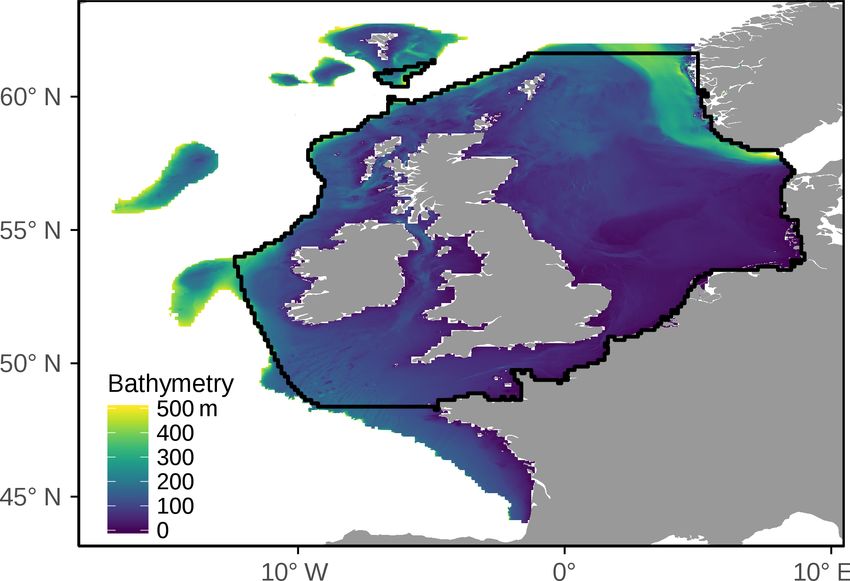
R. J. Wilson et al.: Maps of the north-west European Continental Shelf sedimentary environment                                           111

Table 1. Data products created at a spatial resolution of 0.125◦ by 0.125◦ .

             Variable                    Description                                                                      Unit
             Mud, sand and gravel %      Percentage of surface sediment on seabed composed of mud, sand and gravel        %
             Whole-sediment D50          Median grain size of the whole sediment                                          mm
             Sand D50                    Median grain size of the sand fraction of sediment                               mm
             Gravel D50                  Median grain size of the gravel fraction of sediment                             mm
             Porosity                    Porosity of sediment
             Permeability                Permeability of sediment                                                         m2
             Rock %                      Percentage of area made of up of surface rock or rock in top 50 cm               %
             POC                         Carbon content of organic sediment                                               %
             TN                          Nitrogen content of organic sediments                                            %
             Orbital velocity            Maximum and mean seabed wave orbital velocity                                    m s−1
             Tidal velocity              Maximum and mean depth-averaged tidal velocity                                   m s−1
             Natural disturbance %       Monthly natural disturbance rate of seabed sediments

Table 2. Summary of data sources used in sediment analysis. Datasets 1 (http://www.bgs.ac.uk/geoindex/wms.htm) and 8 (http://www.vliz.
be/vmdcdata/nsbs/) were open access. Datasets 3, 4, 5, 9, 10 and 12 were available from the transnational database of North Sea sediment
data (Valerius et al., 2015), which is a collation of data compiled by the EMODnet-Geology (http://www.emodnet.eu/geology), TOLES
(http://www.belspo.be/belspo/brain-be/projects/TILES_en.PDF) and AufMod (http://www.kfki.de/de/projekte/aufmod) projects. Datasets 2,
6 and 7 were available from institutional contacts. Dataset 11 was downloaded from https://jetstream.gsi.ie/iwdds/index.html.

   No.    Source                                                            Sediment       Whole sediment      Sand    Gravel        Rock
                                                                          percentages                D50        D50      D50      presence
   1      British Geological Survey                                               20 857                 –   13 289        –       20 560
   2      Cefas                                                                    3813               1879        –     1865            –
   3      Federal Maritime and Hydrographic Agency (Germany)                      20 629                 –        –        –            –
   4      Geological Survey of Denmark and Greenland                                 475                 –        –        –        1594
   5      Geological Survey of the Netherlands                                     6346                  -        -        -        5774
   6      Geopotenzial Deutsche Nordsee                                                –                 –        –        –          862
   7      INFOMAR                                                                  1392                  –        –        –            –
   8      Marine Scotland                                                          1214               1214        –        –            –
   9      Marine Scotland(2)                                                           –               898        –        –            –
   10     North Sea Benthos Survey                                                     –               219        –        –            –
   11     Rikswaterstaat (Ministerie van Infrastructuur en Milieu; the             6114                  –        –        –            –
          Netherlands)
   12     Royal Belgian Institute of Natural Sciences                              3433                  –        –         –           –
          All data                                                                64 273              4210   13 289     1865       28 974

will have negligible natural disturbance rates. Data products                  2. In areas where we have data, we spatially interpolate the
were created with a spatial resolution of 0.125◦ longitude by                     relevant statistic onto the study grid.
0.125◦ latitude and are listed in Table 1.
   Seabed sample coverage of this shelf region is highly het-                  3. Using observations, we developed random forest (RF)
erogeneous with large expanses of the domain lacking ac-                          models to predict sediment composition using wave and
cessible data. Hence, our strategy was to fill these voids in                     tidal velocities, bathymetric properties of the seabed and
the sample coverage with statistically modelled values. The                       distance from the coast.
steps involved in mapping the sedimentary environment were
                                                                               4. We then used RF-predicted values to infill regions of
therefore as follows.
                                                                                  the mapping domain where the observed data density
                                                                                  was insufficient for direct gridding.
  1. Sediment data from a number of sources (Table 2) were
     compiled to create a composite dataset of mud, sand                       5. Sediment porosity and permeability at each map grid
     and gravel percentages, rock cover, carbon and nitrogen                      point were derived from the whole-sediment median
     content of sediments, and median grain sizes.                                grain size using empirically based relationships assem-
                                                                                  bled from literature data.

www.earth-syst-sci-data.net/10/109/2018/                                                       Earth Syst. Sci. Data, 10, 109–130, 2018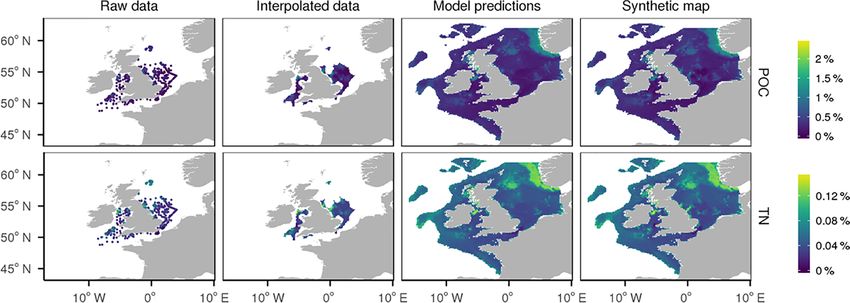
112                        R. J. Wilson et al.: Maps of the north-west European Continental Shelf sedimentary environment

Figure 2. Locations with field estimates of each seabed sediment parameter. Data sources are listed in Table 2.

  6. The natural disturbance rates of sediments at each grid-           were downloaded from the http://www.vliz.be/vmdcdata/
     ded location were then calculated from wave and cur-               nsbs/ website. In total there were 219 records of the whole-
     rent bed shear stress and grain size estimates using sed-          sediment median grain size. These data are available as sep-
     iment dislocation theory.                                          arate webpages for each location and we used the rvest pack-
                                                                        age in R to convert the html code into columned csv format.
                                                                           The Centre for Environment, Fisheries and Aquaculture
2.2     Data sources                                                    Science (Cefas) provided sediment data which included the
2.2.1    Raw sediment data and processing                               mud, sand and gravel percentages and the distribution of sed-
                                                                        iments by grain size. Data provided by Cefas covered a large
We compiled data on the sediment composition of the seabed              part of English and Welsh waters. In total, Cefas provided
from a large number of sources. Our analysis uses the follow-           3814 records of mud, sand and gravel percentages and sedi-
ing data: mud, sand and gravel percentages, rock cover and              ment distribution. However, to provide a consistent estimate
the median grain size of the whole sediment, sand fraction              of sediment type we restricted our analysis to sediments anal-
and gravel fraction. The data sources are summarized in Ta-             ysed using laser methodology and from the top 10 cm of the
ble 2 and the geographic locations where sediment data were             seabed. This resulted in a total of 1879 sediment records be-
available are shown in Fig. 2.                                          ing used. Cefas did not provide estimates of median grain
   The British Geological Survey (BGS, 2013) provides mud,              size. We therefore calculated the median grain size as fol-
sand and gravel percentages and the median grain size of the            lows. For the sediment record at each location, a cumulative
sand fraction for locations in most of the United Kingdom’s             curve of sediment weight percentage was calculated. We then
territorial waters. Data were downloaded from the BGS web-              calculated the median point of this curve and classified this
site using the offshore GeoIndex tool (http://www.bgs.ac.uk/            as the median grain size. This was carried out for the entire
geoindex/wms.htm). The raw BGS dataset included 26 259                  sediment and also for the gravel fraction.
records of sediment composition. However, to provide a con-                Two datasets were provided by Marine Scotland. The
sistent measure of mud, sand and gravel content we only used            first included mud, sand and gravel percentages and whole-
grab samples. This reduced the total number of records of               sediment median grain sizes for a large part of the North Sea.
sediment percentages and sand D50 records to 20 857 and                 In total, this dataset had 1214 sediment records. The second
13 289 respectively.                                                    dataset included estimates of the median grain size of the
   An extensive dataset of surface mud, sand and gravel                 combined mud and sand fraction. These grain size data were
percentages was compiled for the transnational database of              not directly usable, so we filed out samples in which the per-
North Sea sediments (Valerius et al., 2015). This provides              centage of gravel was small enough that the median grain
36 997 records of sediment composition, with data coming                size of the mud–sand fraction was close to that of the whole
from historical records of the Federal Maritime and Hydro-              sediment. To do this we analysed Cefas data and established
graphic Agency (Germany), the Geological Survey of Den-                 that when the whole-sediment D50 is calculated with and
mark and Greenland, the Geological Survey of the Nether-                without the gravel fraction for sediments with less than 10 %
lands, Rikswaterstatt (the Netherlands), and the Royal Bel-             gravel, there is negligible difference between the estimates of
gian Institute of Natural Sciences.                                     D50 . We therefore used the BGS dataset to identify regions
   Records of whole-sediment median grain size were avail-              where the gravel fraction was below 10 %. This was carried
able from the North Sea Benthos Survey (NSBS) (Basford                  out by first calculating the number of BGS observations in
and Eleftheriou, 1988; Basford et al., 1993). NSBS data

Earth Syst. Sci. Data, 10, 109–130, 2018                                                   www.earth-syst-sci-data.net/10/109/2018/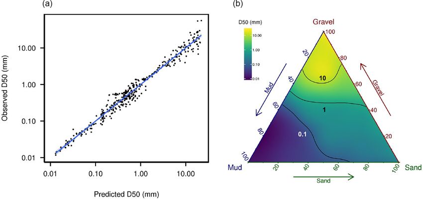
R. J. Wilson et al.: Maps of the north-west European Continental Shelf sedimentary environment                               113

each 0.5◦ N by 1◦ W cell. We excluded cells with fewer than           Borehole records provide reliable records of the rock com-
10 observations. We then further excluded all cells in which       position of the seabed and the layers below it. German
more than 10 % the observations had 10 % of higher gravel          borehole data are available from the Geopotenzial Deutsche
content. In these regions we accepted the Marine Scotland          Nordsee project. The http://www.gpdn.de/ website provides
data as a reasonable estimate of the whole-sediment D50 .          visual records of borehole logs at a large number of loca-
   The Infomar project (http://www.infomar.ie) is mapping          tions in German territorial waters in the North Sea. A total
the seabed in Ireland’s territorial waters. It has compiled a      of 862 records were visually inspected and we found no evi-
historical dataset of grab samples which show the surface          dence of rock at or near the surface in any record. The Geo-
mud, sand and gravel percentages in many locations in Irish        logical Survey of the Netherlands provides extensive bore-
waters. Data were downloaded in shape file format from the         hole data. These were downloaded as individual text files
https://jetstream.gsi.ie/iwdds/map.jsp website. In total, there    from the https://www.dinoloket.nl/en/subsurface-data web-
were 1392 records of surface sediment composition.                 site. Each text file provided a record of the sediment type
                                                                   in each layer of the borehole in a consistent format. We first
2.2.2   Rock data
                                                                   identified whether there was rock in the top 50 cm of any of
                                                                   the core records and found none. We therefore found no ev-
Our aim was to classify locations as non-rock, rock at sur-        idence of surface rock in Dutch waters. The Geological Sur-
face (i.e. approximately the top 10 cm of sediment) and rock       vey of Denmark and Greenland provides borehole data for
in the approximately top 50 cm of sediment and to map the          Danish waters in the North Sea. Data were available from the
percentage of surface area in each rock classification. His-       http://www.geus.dk website. Each borehole record is avail-
torically, areas have only been mapped in a discrete fashion       able as a separate webpage, and we therefore used the R
(e.g. the British Geological Survey’s Digirock map; Gafeira        package rvest to save the relevant html code and convert the
et al., 2010), with relatively broad areas placed in one rock      depth profile of sediment type to csv format. We were then
category or another. Further, there are no published large-        able to identify the sediment type in the top 10 and 50 cm at
scale datasets explicitly identifying whether locations have       each location.
rock at or near the sea floor. We therefore created a compos-
ite dataset using historical survey logs for British territorial   2.2.3   Carbon and nitrogen content
waters and borehole records for the territorial waters of Den-
mark, Germany and the Netherlands.                                 Diesing et al. (2017) showed that the carbon content of sed-
   The British Geological Survey provides a database of            iment could be credibly predicted based on a series of en-
downloadable historical logs of sediment sampling sur-             vironmental predictors. Here we take a similar approach to
veys (available from http://www.bgs.ac.uk/geoindex/wms.            the predictive mapping of the carbon and nitrogen content
htm) with good spatial coverage for British territorial waters.    of sediments. Particulate organic carbon (POC) and total ni-
These logs come in the form of scanned PDFs, and they pro-         trogen (TN) content were downloaded from the Cefas Data
vide written summaries of each sampling event. The analysis        Hub (https://doi.org/10.14466/CefasDataHub.32) and taken
was restricted to corer records, which typically provided suf-     from Serpetti et al. (2012). It is clear that carbon and ni-
ficient information to determine if there was strong evidence      trogen levels in sediment are strongly determined by mud
of rock at or near the seabed. Grab sample survey data were        content (Serpetti et al., 2012), and each record of carbon
initially analysed; however, the use of grab sample records        and nitrogen content is associated with a field estimate of
will underestimate rock levels as the grab can return sedi-        mud content. We therefore used mud as a predictor. How-
ment despite there being rock at or close to the surface. We       ever, the mud measurements in the Cefas dataset alternate
therefore ignored grab samples.                                    between using laser and sieve methodology and therefore do
   Before analysing the PDFs we created the following cate-        not provide consistent and comparable estimates of mud con-
gories for the records: (1) evidence shows there is no rock at     tent. The Cefas dataset contained 182 sediment samples for
the location; (2) written logs are consistent with rock at the     which the mud content was estimated using laser and sieve
surface or rock covered by a thin skin of sediment (approxi-       methodology, which showed a strong statistical relationship
mately 10 cm); (3) written logs show that there is probably a      between each measure. We therefore converted each sieve
significant layer of sediment covering rock; (4) ambiguous or      estimate of mud content to a laser equivalent using a statisti-
an unreadable record. A Python script was written that will        cal relationship modelled using the lm function in R (laser
move through each PDF and allow an analyst to classify it.         mud = 3.157 × (sieve mud)0.7225 , p value: < 2.2 × 10⁻¹⁶ ,
This process was randomized to ensure there was no spatial         r 2 = 0.93) (Fig. 3).
bias in classification error. In total there were 20 709 initial
PDFs. Of these 149 could not be classified as rock or non-
rock and were discarded. There were 18 871 records with no
evidence of rock, 747 with evidence of rock at or near the
surface and 942 records showing rock in the top 50 cm.

www.earth-syst-sci-data.net/10/109/2018/                                             Earth Syst. Sci. Data, 10, 109–130, 2018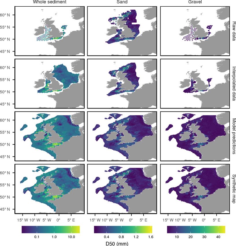
114                      R. J. Wilson et al.: Maps of the north-west European Continental Shelf sedimentary environment

2.2.4   The physical environment                                 mean square shear stresses for waves plus currents were used.
                                                                 The calculation of bed shear stress requires the bathymetry,
Depth-averaged tidal velocities were calculated as follows.
                                                                 depth-averaged current speed, current direction, significant
For most of the study region tidal velocities were taken from
                                                                 wave height, wave period and wave direction.
the output of the Scottish Shelf Model, which is an imple-
                                                                    For the statistical modelling of sediment composition
mentation of the unstructured, finite-volume 3-D hydrody-
                                                                 we used EMODnet bathymetry data. These have a spa-
namic model FVCOM. The spatial domain of this model
                                                                 tial resolution of 1/8 arcmin by 1/8 arcmin and were down-
covers approximately 80 % of our study domain (Fig. 1). A
                                                                 loaded from the EMODnet website (http://www.emodnet.eu/
full description of the model is provided by De Dominicis
                                                                 bathymetry/). Data processing and calculations were carried
et al. (2017), and here we use the same model run described
                                                                 out in R using the packages dplyr (Wickham et al., 2017) and
therein. A 1-year climatology (for the years 1990–2014) of
                                                                 Rcpp (Eddelbuettel et al., 2011).
atmospheric forcings was used to run the model.
   For the rest of the model domain we derived tidal veloci-
ties as follows. The Oregon State University Tidal Prediction    2.3   Spatial gridding and predictive modelling
Software (OTPS) is a well-known open-source barotropic
                                                                 The synthetic maps of mud, sand and gravel percentages, and
tidal model based on the Oregon State University tidal in-
                                                                 rock cover were created as follows. First we identified re-
version of TOPEX/POSEIDON altimeter data and tide gauge
                                                                 gions where a statistical interpolation of the relevant param-
data (Egbert et al., 2010). This model was used to derive the
                                                                 eter would give a reasonable estimate across that region. In
relevant tidal components. The model can be obtained from
                                                                 other regions we used statistical models to predict the param-
http://volkov.oce.orst.edu/tides/otps.html. We obtained a re-
                                                                 eter. We assume that the environmental drivers of sediment
gional tidal solution using the Oregon State University Tidal
                                                                 composition are consistent across space.
Inversion Software (OTIS) with a spatial resolution of 1/30◦ .
                                                                    Sampling coverage of sediment composition covered al-
The model satisfies the depth-integrated two-dimensional
                                                                 most all of the North Sea, the United Kingdom’s territorial
shallow water equations describing momentum balance as
                                                                 waters and parts of Ireland’s territorial waters (Fig. 2). Obser-
follows:
                                                                 vations almost universally come from sampling programmes
∂u                                                               that aimed to provide consistent spatial coverage of a specific
   + f × u + u · ∇u + F + AH ∇ 2 u = −g∇(η − ηEQ ), (1)          region (e.g. the North Sea Benthos Survey; Basford et al.,
∂t
                                                                 1993), and parameters can be interpolated in those regions.
and volume conservation                                          These regions were selected by creating an alphahull around
    ∂η                                                           each unique set of coordinates using the R package alphahull
−      = ∇ · (H + η)u,                                     (2)   (Pateiro-l and Rodr, 2010). An alphahull is a convex envelope
    ∂t
                                                                 around the data points which will exclude areas outside the
where η is sea surface elevation, u is the horizontal veloc-     sampled regions and exclude large holes in the data coverage.
ity vector, f is the Coriolis parameter, F is the fractional     Data were first interpolated onto a 1/16◦ by 1/16◦ grid and
damping, AH is an eddy coefficient, which is assumed to be       then means were calculated for each 0.125◦ by 0.125◦ cell.
constant, H is bathymetry and ηEQ is the equilibrium tide        Parameters were spatially interpolated using bilinear spline
allowing for the body tide, tidal self-attraction and loading.   interpolation using the interpp function from the R package
   Wave conditions were acquired from the ERA-Interim re-        akima (Akima and Gebhardt, 2016).
analysis (Dee et al., 2011). Significant wave height, mean          For areas outside the alphahulls we used random forest
wave period and mean wave direction were downloaded from         (Liaw and Wiener, 2002) models to predict each parameter.
the ECMWF website at http://www.ecmwf.int/en/research/           This class of model has been used to predict seabed sedi-
climate-reanalysis/. The ERA-Interim reanalysis has a spa-       ments (Diesing et al., 2014; Huang et al., 2012; Li et al.,
tial resolution of approximately 79 km and a temporal res-       2011) and carbon and nitrogen content (Diesing et al., 2017).
olution of 6 h. Orbital velocities at the seabed were calcu-     Random forest was developed by Breiman (Breiman, 2001).
lated using the equations of Soulsby (2006), and the relevant    It is an ensemble-based modelling approach that makes no
equations are given in this paper’s Appendix. Bathymetry         assumptions about the form of the relationships between
for the wave and tidal model runs was attained from the          predictor and response variables, does not require exten-
high-resolution (30 arcsec) General Bathymetric Chart of the     sive parameterization, performs internal cross-validation and
Oceans (GEBCO). With the exception of the Scottish Shelf         avoids over-fitting. Random forest takes an ensemble-based
Model output we used 2012 as the year for analysis of wave       approach to regression. This is carried out by first growing
and tidal conditions.                                            a number of regression trees (Loh, 2011). Each tree is com-
   To calculate the bed shear stress we used the equations       posed of a bootstrapped sample from, and of the same size
of Soulsby and Clarke (2005) under combined wave and             as, the fitting data. Bootstrapped samples are drawn with re-
currents conditions on smooth and rough beds. This set of        placement. Each split in the tree-building process only uses
equations is reproduced in the Appendix to this paper. Root      a subset of the predictor variables. Splitting the trees in this

Earth Syst. Sci. Data, 10, 109–130, 2018                                          www.earth-syst-sci-data.net/10/109/2018/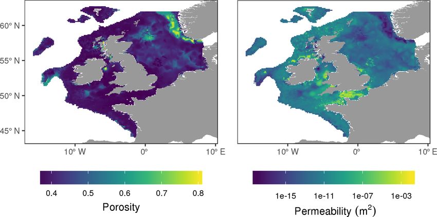
R. J. Wilson et al.: Maps of the north-west European Continental Shelf sedimentary environment                               115

way reduces the dominance of individual variables and thus        erarchical, High-resolution Geography (GSHHG) Database
decorrelates the trees, making the trees less variable and        (Wessel and Smith, 1996). Distance of each data point from
more reliable (James et al., 2013). The average across all        the coast was then calculated using the R package geosphere
trees is then used for predictions. This ensemble averaging       (Hijmans et al., 2012).
makes random forest robust to over-fitting (Breiman, 2001).          Smoothness of the seabed will influence seabed distur-
   The observed mud, sand and gravel percentages summed           bance and sediment accumulation and is likely an indica-
to 100. However, there is no guarantee that separately pre-       tor of the existence of rocky outcrops. We therefore included
dicted mud, sand and gravel percentages will sum to 100.          measures of seabed roughness as predictors in each random
We therefore predicted the mud, sand and gravel percent-          forest. A number of methods exist to quantify the roughness
ages separately and then a multiplier was applied to each         of the seabed (Wilson et al., 2007). However, many of them
prediction so that the predictions were adjusted to total 100.    are not independent of the slope of the sea floor and are ar-
Random forests were created in R using the ranger package         guably not purely measures of roughness. For example, the
(Wright and Ziegler, 2017), which is a computationally effi-      standard deviation of bathymetry would classify a steeply
cient implementation of random forest for high-dimensional        sloping but smooth part of a continental shelf as being very
data. The number of trees was set to 2000, with mtry set to 3.    rough. We therefore used the standard deviation of slope and
   A similar process was carried out for median grain sizes       the standard deviation of the residual topography as predic-
and carbon and nitrogen content. Grain size data were avail-      tors in the random forests. Residual topography is the differ-
able for large parts of the United Kingdom’s territorial wa-      ence between the bathymetry at a specific point and the mean
ters and some parts of the North Sea, while carbon and nitro-     bathymetry within a specified spatial window. The residual
gen content were exclusively available in parts of the United     topography was calculated using a 25-cell moving window.
Kingdom’s territorial waters (Fig. 2). First we used the al-      First the mean bathymetry was calculated within each win-
phahull approach to identify regions where we can inter-          dow. The standard deviation of residual topography (σ ) was
polate the parameter. We then used statistical models (dis-       then calculated
                                                                             qP using the formula of Cavalli et al. (2008):
cussed in Sect. 2.3.1) to predict each parameter. In each case    σ = 1/25        25            2
                                                                                  i=1 (xi − xm ) , where xi is the bathymetry in a
the sediment percentage maps discussed above were used as         specific cell in the moving window and the respective mov-
predictors in the mapping exercise. Maps and figures were         ing window mean bathymetry. Slope was calculated using
produced using the R package ggplot2 (Wickham, 2016) and          the slope function from the R package SDMTools (VanDer-
ternary diagrams were produced using the R package ggtern         Wal et al., 2014). We then calculated the standard deviation
(Hamilton, 2017).                                                 of slope in a similar 25-cell moving window.
                                                                     The above predictors were used for the mud, sand and
2.3.1   Environmental predictors for random forest                gravel percentage and rock cover models. For the models
        models and model validation                               of carbon and nitrogen content we also included chloro-
                                                                  phyll, salinity and seabed temperature. Carbon and nitro-
The environmental predictors used for the random forest           gen content are influenced by biological activity and should
models that predicted mud, sand and gravel percentage, rock       thus be influenced by primary production levels and tem-
cover, and carbon and nitrogen content are listed in Table 3.     perature at the seabed. The MetO-NWS-REAN-PHYS-bed-
Predictors were chosen based on a review of evidence on the       daily reanalysis was used for seabed temperature. These data
environmental influences on the seabed and the requirement        were downloaded from the Copernicus Marine Environmen-
that data were available at the necessary spatial resolution.     tal Monitoring Service website (http://marine.copernicus.eu/
   Tidal and wave energy levels at the seabed should strongly     services-portfolio/access-to-products/). Daily seabed tem-
influence mud, sand and gravel percentages. Large grain           peratures from 1995–2014 were interpolated onto each lo-
sizes require more energy to dislodge from the seabed, and        cation and an annual climatology was calculated for each
therefore high bed shear stress is associated with increases in   model grid point. Climatological (1997–2015) annual mean
average grain size and reductions in mud content (Ward et al.,    chlorophyll (mg m−3 ) data were derived from the level 4
2015; Heath et al., 2016). There is scarce evidence to de-        North Atlantic chlorophyll concentration from satellite ob-
termined if seabed composition is influenced by year-round        servations reprocessed data product, which is available from
bed shear stress or individual high-energy events. We there-      the Copernicus website. Proximity to river outflows likely in-
fore used mean and maximum annual tidal and wave orbital          fluences levels of carbon and nitrogen, and salinity levels act
velocities as predictors in the models of sediment composi-       as a proxy for this. We therefore calculated an annual cli-
tion and carbon and nitrogen content. The supply of sediment      matological mean (1985–2014) of salinity from the MetO-
from river discharges and coastal erosion influences seabed       NWS-REAN-PHYS-monthly-SAL reanalysis product avail-
sediment composition and carbon and nitrogen. We therefore        able from the Copernicus website.
included distance from the coast as a model predictor. The           Our methodology involves predicting the sedimentary en-
distance from the coast was calculated as follows. Shape files    vironment in geographically distinct regions. We therefore
of coasts were attained from the Global Self-consistent, Hi-

www.earth-syst-sci-data.net/10/109/2018/                                            Earth Syst. Sci. Data, 10, 109–130, 2018
116 R. J. Wilson et al.: Maps of the north-west European Continental Shelf sedimentary environment
Table 3. Predictors used for statistical models for predicting sediment parameters. When mud, sand and gravel percentages and whole-
sediment median grain sizes were used as predictors, raw field data were used in the creation of the statistical models, whereas the synthetic
maps created in this study were used for model predictions.
Predictor used?
Predictor Unit Mud, sand, gravel, rock POC, TN D50 s Porosity, permeability
Maximum and mean wave orbital velocity m s−1 Y Y – –
Max. and mean depth-averaged tidal velocity m s−1 Y Y – –
Bathymetry m Y Y – –
Standard deviation of residual topography m Y Y – –
Standard deviation of slope ◦ Y Y – –
Distance from coast km Y Y – –
Mean annual salinity - Y Y – –
Mean annual chlorophyll mg m−3 Y Y – –
Mud percentage % – Y Y –
Sand percentage % – – Y –
Gravel percentage % – – Y –
Total D50 % – – – Y
tested the ability of random forest models to do this credi-
bly by using a cross-validation technique involving spatially
disaggregated training and test datasets. Spatial disaggrega-
tion has been shown to be a reasonable method to avoid the
excessive overconfidence that can possibly result from other
training and testing methodologies of spatial models (Bahn
and McGill, 2013; Roberts et al., 2017). The cross-validation
method was as follows. We chose to use the spatial block-
ing method from Roberts et al. (2017). This places data into
consistently sized and spatially separate blocks or bins. We
chose to bin data at a resolution of 1◦ longitude by 1◦ lat-
itude. We then used 100 iterations in which each bin was
randomly assigned to training and test datasets. In each iter-
ation the random forest was trained using the training dataset
and this model was then used to predict the relevant parame-
ter using the test data. We therefore evaluated the predictive
ability of the model by calculating the mean value of each
statistic in the test data for each 0.125◦ by 0.125◦ cell. The
number of observations, and thus the observation reliability,
in each cell varies significantly. We therefore calculate the
weighted r 2 between predicted and observed values in each
cell, with the number of observations used as the weighting Figure 3. The relationship between mud estimated from laser and
sieve methodology for the same samples. For estimates of car-
value. Weighted correlation coefficients were calculated us-
bon and nitrogen content with only sieve-based estimates of mud
ing the function corr from the R package boot (Canty, 2002).
content, we estimated what the mud percentage would be when
For the full predictive models over the entire European shelf calculated using laser methodology. The dashed red line shows
we retrained the random forests using all available data. this relationship (laser mud = 3.157 × (sieve mud)0.7225 , p value:
< 2.2 × 10⁻¹⁶ , r 2 = 0.93).
2.3.2 Median grain sizes
Sufficient median grain size data were available to provide
a spatial interpolation of whole-sediment D50 in most of the
North Sea and large parts of the English Channel and Irish polation and interpolating solely within the alphahull which
Sea. We therefore interpolated whole-sediment D50 in these surrounds the relevant data points. Outside the alphahulls we
regions. This was carried out in the same way as for the dis- predict the relevant D50 using the mud, sand and gravel per-
tribution of sediment percentages using bilinear spline inter- centages in the synthetic maps created in this study.
Earth Syst. Sci. Data, 10, 109–130, 2018 www.earth-syst-sci-data.net/10/109/2018/R. J. Wilson et al.: Maps of the north-west European Continental Shelf sedimentary environment 117
Table 4. Published literature with porosity estimates. These data
were used to statistically model porosity in terms of whole-sediment
median grain size.
Reference Region
Wiesner et al. (1990) North Sea
Lohse et al. (1993) North Sea
Ruardij and Van Raaphorst (1995) North Sea
Serpetti et al. (2012) North Sea
sand and gravel percentages are accounted for using a ten-
sor product smooth (te). As with the sediment percentages,
data were split into training and testing data. We randomly
selected 70 % of the data and used it as the training data, and
then used the remaining 30 % as the test data. Likewise, the
final predictive model was created using all of the data.
For the sand and gravel fractions we used a GAM of the
form D50 ∼ te(mud, sand, gravel), with a log-link function to
ensure predictions were never negative. Finally, a small num-
ber of predictions for the sand and gravel D50 were outside
the grain size boundaries for gravel or sand respectively. In
these cases we forced the modelled D50 to be the largest or
smallest possible grain size where appropriate. General addi-
tive models were created using the R package mgcv (Wood,
Figure 4. (a) Assembled data on sediment porosity and median
2001).
grain size (filled circles) and the fitted relationship (solid line).
(b) Annual average permeability m−2 of sediments from seven sites
off the north-east coast of Scotland; data from Serpetti et al. (2016). 2.3.3 Porosity and permeability
The porosity and permeability of sediments are quantita-
tively related to grain size distribution, with coarser-grained
In contrast to the mud, sand and gravel percentages, we sediments having lower porosity and higher permeability.
chose not to predict median grain sizes using environmen- We evaluated the relationship between porosity and whole-
tal variables. Predicting both the sediment percentages and sediment median grain size by compiling published data (Ta-
median grain sizes separately is likely to result in contradic- ble 4). Porosity is conventionally expressed as the percentage
tory predictions. For example, a model might predict a much volume of sediment occupied by void spaces of water. How-
higher median grain size than is possible given the predicted ever, some data (Wiesner et al., 1990) expressed water per-
sediment percentages. We therefore chose to create a statis- centage by weight. In this case we converted the water con-
tical model which predicts the median grain size using mud, tent data (by weight) to porosity assuming a solid material
sand and gravel percentages. density of 2.65 g cm−3 and a fluid density of 1.025 g cm−3 .
The median grain size of the gravel fraction has previ- There was a sigmoidal relationship between log-transformed
ously been shown to relate strongly to the mud to sand ra- porosity and log10 grain size (mm). We therefore fitted a lo-
tio (Aldridge et al., 2015). We therefore chose to model the gistic relationship between them using Nelder–Mead opti-
whole-sediment D50 , the sand D50 and the gravel D50 in re- mization in the optim package in R (Fig. 4). This equation
lation to mud, sand and gravel percentages. In all cases we is shown below and the parameters are given in Table 5.
used general additive models (GAMs) (Wood, 2006), which
marginally outperformed random forests in terms of predic- 1
log10 porosity = p1 + p2 −(log10 D50−p3 )
(3)
tive ability. p4
1+e
The median grain size of the whole sediment varied by
4 orders of magnitude. Consequently, a GAM which uses To our knowledge the best dataset available on the relation-
the D50 unaltered was incapable of credibly predicting the ship between whole-sediment permeability and median grain
D50 for the small-grained muddy sediments. We therefore size is that of Serpetti et al. (2016). This dataset covered
used the following log transformation for the general additive muddy sand, sand and mixed sediments sampled at approx-
model of the total sediment median grain size; log10 (D50 ) ∼ imately monthly intervals over 1 year at seven sites off the
te(mud, sand, gravel), where the interactions between mud, east coast of Scotland. Permeability and median grain size
www.earth-syst-sci-data.net/10/109/2018/ Earth Syst. Sci. Data, 10, 109–130, 2018118 R. J. Wilson et al.: Maps of the north-west European Continental Shelf sedimentary environment
Table 5. Fitted values and standard errors of the four parameters determined by the wave and tide conditions and the whole-
required for the function relating sediment porosity to median grain sediment D50 . However, for the mud, sand and gravel fraction
size. the critical threshold is determined by the D50 of the relevant
fraction.
Parameter Fitted value Standard error We therefore estimate natural disturbance using the fol-
p1 −0.436 0.023 lowing procedure for each day of the year.
p2 0.366 0.050
p3 −1.227 0.063 1. Calculate the bed shear stress at each 15 min time inter-
p4 −0.270 0.046 val using equations shown in this paper’s Appendix and
the whole-sediment D50 .
2. Determine the critical threshold at each time step for
were measured on cores from the upper 5 cm and upper
mud, sand and gravel using the respective D50 and
10 cm of the seabed at each site. Most sediments are sam-
Eq. (A50).
pled at a depth of 10 cm and we therefore chose to only map
permeability at this depth. The differences in annual average 3. Percentage of area disturbed = (Mud% × Muddist ) +
permeability (m−2 ) can be explained using a power function (Sand% × Sanddist ) + (Gravel% × Graveldist ), where
of median grain size (D50 , mm) (r 2 = 0.999 for 10 cm cores). Muddist , Sanddist , Graveldist denote whether the Shields
The equation was as follows: stress exceeded the critical threshold for mud, sand and
gravel respectively.
Permeability = 10−9.213 D4.615
50 (10 cm cores).
We follow Aldridge et al. (2015) and use a 1-day time win-
Porosity and permeability were mapped across the study re- dow to classify disturbance events. Monthly disturbance rates
gion using the above equations and the synthetic map median are then calculated by aggregating the areas disturbed in each
grain size. day of the month. It is important to note that the modelled
We then used the porosity estimates and the maps of POC disturbance rate ignores the existence of rock at the surface.
and TN to derive additional maps of the density of carbon We are therefore only modelling the disturbance rate in re-
(kg C m−2 ) and nitrogen (kg N m2 ) stored in the surface sedi- gions with sediment cover.
ment layer across the shelf. This was derived from the carbon
and nitrogen percentages of sediment and porosity values us-
ing the following equation. 3 Results
Carbon density (kg m−2 ) 3.1 Sediment percentages and median grain sizes
= POC × sediment depth (m) Figure 5 shows the derivation of the synthetic map of sedi-
× Dry sediment density (kg m −3
) × (1 − porosity) ment percentages. The interpolated map shows that mud (re-
gions with greater than 50 % mud) is largely concentrated
= TN × 0.1 × 2650 × (1 − porosity)
in the deep Norwegian Trench, an area in the north-western
Nitrogen density (kg m−2 ) North Sea, part of the western Irish Sea and in patches on
= TN × 0.1 × 2650 × (1 − porosity) the Scottish west coast. Sandy sediments (greater than 50 %
sand) dominate in the North Sea, except for those areas with
high mud and a small region on the south-eastern English
2.3.4 Natural disturbance
coast with high gravel levels. High gravel levels are seen ex-
We modelled the extent to which the surface layers of the clusively in shallow coastal regions, with most of the English
sediment were disturbed by waves and tides during the year. Channel having more than 50 % gravel.
Disturbance was defined as an event which results in physi- The predictions of the random forest models reproduce
cal movement of the surface sediments due to the effects of the large-scale geographic patterns of sediment composition.
bed shear stress. We then estimated the average percentage of The R 2 values of the predictions of mean sediment percent-
area disturbed per month in each 0.125◦ by 0.125◦ cell over age in each 0.125◦ by 0.125◦ grid cell on the test data were
our model region. We assumed that sediments are mobilized 0.444, 0.412 and 0.476 for mud, sand and gravel percentages
when the bed shear stress exceeds a critical Shields threshold respectively. The models pick up most of the key geographic
and that this threshold is given by the equation provided by features revealed by the spatially interpolated map. The high
Wilcock et al. (2009). levels of mud in the Norwegian Trench, west of the Isle of
Disturbance could be heterogeneous in space and time Man and the region of the northern North Sea are reproduced.
within each of our 0.125◦ by 0.125◦ cells due to variations Regions of the western North Sea with relatively high mud
in grain size and shear stress. We accounted for this het- levels are also well represented. Similarly, the model predicts
erogeneity as follows. The bed shear stress on the seabed is the existence of relatively high levels of mud south of Ireland.
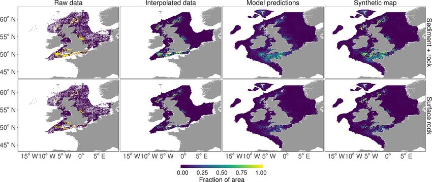
Earth Syst. Sci. Data, 10, 109–130, 2018 www.earth-syst-sci-data.net/10/109/2018/R. J. Wilson et al.: Maps of the north-west European Continental Shelf sedimentary environment 119 Figure 5. The derivation of the synthetic map of sediment percentages. The interpolated map uses bilinear spline interpolation using sediment data over the region. The random forest map predicts the sediment percentages using a random forest model which relates the percentage to the bed shear stress and the distance to the coast. The synthesized map merges the two by using spatial interpolations where we have data and the random forest predictions where we do not. The GAM of whole-sediment D50 created using the train- regions such as that in the north-western North Sea. The me- ing dataset performed well against the test data. R 2 was 0.85 dian grain size of the sand fraction can be interpolated for on the D50 values and 0.95 on the log10(D50 ) values. This most British territorial waters and is highest in regions which model had an R 2 of 0.98. Figure 6 shows the modelled re- are predominantly gravelly. The median grain size of the lationship between percentages of mud, sand and gravel and gravel fraction can only be interpolated for parts of south- the median grain size of the whole sediment. The GAM re- ern British territorial waters, and it is highest in regions of lating the sand D50 to the mud, sand and gravel percentages, high gravel content. which was trained on the training dataset, had an R 2 0.42 Figure 8 shows the derived maps of porosity and perme- when compared with the test data. The R 2 for the GAM re- ability. Porosity is similar across most regions, with the ex- lating the gravel D50 to the mud, sand and gravel percentages ception of the muddy areas in the Norwegian Trench, north- was 0.38. western North Sea and the Irish Sea. Permeability varies by Figure 7 shows the derivation of the synthetic maps of me- 18 orders of magnitude. It is highest in the gravelly regions dian grain sizes. Whole-sediment median grain size can be in the English Channel and some coastal regions, and it is interpolated for most of the North Sea, English Channel, and lowest in muddy regions. the Irish and Celtic seas. It varies by approximately 3 or- The synthetic maps of rock cover are shown in Fig. 9. Ob- ders of magnitude, with median grain sizes above 10 mm in served data indicate that the eastern North Sea is almost en- the gravelly regions in the English Channel and other coastal tirely free of surface rock. There are large concentrations of regions and median grain sizes close to 0.01 mm in muddy surface rock in the English Channel, south-west of England, www.earth-syst-sci-data.net/10/109/2018/ Earth Syst. Sci. Data, 10, 109–130, 2018
120                        R. J. Wilson et al.: Maps of the north-west European Continental Shelf sedimentary environment

Figure 6. (a) Predictions of a GAM that relates whole-sediment D50 to the mud, sand and gravel percentages. (b) Relationship between
total sediment median grain size and percentage of mud, sand and gravel. The relationship was derived using a general additive model which
relates the D50 to the mud, sand and gravel percentage.

Figure 7. Summary of the derivation of the synthetic median grain size maps. Where we have sufficient median grain size data we spatially
interpolated a map of D50 . In other locations we used the synthetic map of mud, sand and gravel percentages and a GAM which relates the
D50 to the mud, sand and gravel percentages to predict the D50 .

Earth Syst. Sci. Data, 10, 109–130, 2018                                                  www.earth-syst-sci-data.net/10/109/2018/
R. J. Wilson et al.: Maps of the north-west European Continental Shelf sedimentary environment                                           121

Figure 8. Maps of porosity and permeability. The relationship between porosity and permeability and median grain size was estimated using
published field data. We then predicted porosity and permeability using the synthetic map of median grain size.

Figure 9. Proportion of area in each rock classification. Areas were classified by whether there was rock at the surface or a surface sediment
layer plus rock in the top 50 cm. Historical survey logs and borehole records were first interpolated to provide a map of rock cover where
we have sufficient data. Random forests were used to predict rock cover elsewhere using wave and tidal velocities, bathymetry, measures of
bathymetry variation and distance from the coast as predictors.

the Bristol Channel and west of the Hebrides Islands on the              content. Therefore the regions of high carbon and nitrogen
west coast of Scotland. The predictions of the random forest             content reflect those of large mud content.
model of rock provide credible large-scale reproductions of
the geographic patterns of rock cover. Predictions of surface            3.2    Natural disturbance
rock and rock in the top 50 cm have r 2 of 0.104 and 0.1991
when compared with mean values in each 0.125◦ by 0.125◦                  Figure 11 shows modelled natural disturbance in each month.
grid cell. The random forest predictions in Fig. 9 reproduce             The deep Norwegian Trench is notable for lacking any dis-
the key rock areas shown by the spatially interpolated map.              turbance year round. Disturbance is highest in the southern
Regions where we rely on predictions are largely rock free,              North Sea where sandy regions on the French, Belgian and
with the notable exceptions of the high-energy English Chan-             Dutch coasts see disturbance events almost on a daily ba-
nel, north-west of France and west of the Faroe Islands.                 sis. There is a notable seasonal pattern in disturbance rates,
   The mapped carbon and nitrogen content of sediment are                with summer months seeing lower disturbance rates, which
shown in Fig. 10. The random forest predictions show close               reflects the lower wind and wave regime in this time period.
agreement with observations. Across 100 iterations in which
training and test data were spatially disaggregated, 70 % of             4     Data availability
data in the training data, there was a mean r 2 of 0.59 and 0.70
between predicted and observed POC and PON respectively.                 The data products listed in Table 1 can been be down-
Carbon and nitrogen content are largely determined by mud                loaded in csv, netcdf and ESRI grid format from

www.earth-syst-sci-data.net/10/109/2018/                                                     Earth Syst. Sci. Data, 10, 109–130, 2018
122                        R. J. Wilson et al.: Maps of the north-west European Continental Shelf sedimentary environment

Figure 10. Derivation of the synthetic maps of particulate organic carbon (POC) and nitrogen (TN). Data were interpolated based on field
observations in areas with good spatial coverage. In other regions, parameters were predicted using a random forest which had mud content
and physical environmental variables as predictors.

Figure 11. Modelled monthly disturbance rate. A disturbance event was defined as a time when the bed shear stress exceeded the threshold
required to move either the mud, sand or gravel portion of the sediment. The monthly disturbance rate was defined as the mean fraction of
the total mud, sand and gravel area disturbed per day.

https://doi.org/10.15129/1e27b806-1eae-494d-83b5-                      we were able to map with high confidence the sediment
a5f4792c46fc (Wilson et al., 2017).                                    composition of the North Sea and British territorial waters,
                                                                       and we were able to make credible statistical predictions
                                                                       of the sediment composition in other regions. The compiled
5   Discussion                                                         datasets of sediment composition and disturbance regime are,
                                                                       as far as we know, the most extensive that exist over such a
The underlying goal of this study was to synthesize large-             large spatial scale. A number of applications exist for these
scale information about the physical environment of the                datasets, including habitat mapping and quantification of an-
seabed, both in terms of the characteristics of sediment and           thropogenic disturbance on the seabed.
the wave and tidal regimes which cause disturbance. Using
field estimates of the sediment composition of the seabed,

Earth Syst. Sci. Data, 10, 109–130, 2018                                                 www.earth-syst-sci-data.net/10/109/2018/
R. J. Wilson et al.: Maps of the north-west European Continental Shelf sedimentary environment 123
Habitat mapping requires knowledge of the composition level of uncertainty. Furthermore, our raw data revealed that
of seabed sediments (Galparsoro et al., 2012), and the maps rock cover shows large levels of heterogeneity. The low num-
we produced can be seen as complementary to previous work bers of samples (1 or 2) available in most 0.125◦ by 0.125◦
(e.g. the EU Mesh project; Vasquez et al., 2015). Existing grid cells means that our available estimates of rock cover
habitat maps typically use discontinuous categories, and the are highly uncertain, which inevitably leads to a model with
continuous nature of the maps we have produced may be ad- lower levels of predictability. Predictive modelling is also
vantageous for some researchers. complex due to the array of conditions that appear to result
in a rocky seabed. The English Channel and Bristol Channel
Limitations and assumptions
are rocky due to the strong tidal energy regime, whereas the
region west of the Hebrides Islands on the Scottish west coast
A simplifying assumption of our study was that sedimentary is relatively rocky due to the existence of rocky outcrops. It
environments are in a state of equilibrium or near equilibrium is also possible that underlying geology plays a key role in
throughout the European Shelf. However, this is unlikely to determining rock levels. A previous study that took a similar
be true everywhere. Ward et al. (2015) have argued that the predictive modelling approach in British waters used infor-
coarser sediments found south-east of Ireland were inherited mation about rock formations as predictors (Diesing et al.,
from prior stress regimes. Furthermore, the Irish Sea has lin- 2015; Downie et al., 2016); however, we were unable to find
ear tidal sand ridges, which are likely relics from an earlier any comparable datasets that covered the entire north-west
more energetic stress regime (Uehara et al., 2006; Scourse European Shelf.
et al., 2009). Reconstructions of historical tidal conditions We excluded the influence of rivers from predictive mod-
on the European Shelf (e.g. Uehara et al., 2006; Neill et al., els because of a lack of large-scale data. However, it is likely
2010, 2009) could potentially be included as model predic- that this is a key influence near large estuaries. This can be
tors in future modelling studies. seen in the high-energy Bristol Channel, where there is both
Our maps of rock area are broadly comparable with the a high level of rock and a relatively high level of mud due
existing hard substrate map for British territorial waters pro- to the contradictory influences of strong tidal currents and
duced by the British Geological Survey (Gafeira et al., 2010). the sediment deposits from the river Severn (McLaren et al.,
Both maps largely draw on historical British Geological Sur- 1993). The influence of river outflows is implicitly captured
vey logs from sea-floor surveys; however, the philosophy and by the inclusion of distance from the coast as a predictor.
motivation of our study differed from that of the British Geo- For example, there is a large increase in the carbon content
logical Survey. The British Geological Survey was motivated of sediments close to coasts, which is likely influenced by
by mapping rocky reef areas for marine conservation plan- sediment deposits from rivers. We therefore cannot rule out
ning purposes. Regions were classified as rock or non-rock, the possibility that certain parameters were over- or under-
which inevitably leads to an overestimation of rock cover if predicted in coastal regions due to the influence of estuar-
analysts assume that all mapped rock regions are made up ex- ies. Similarly, we did not include the potential effects of the
clusively of rock. This is illustrated in the region west of the horizontal transport of sediment by currents (Tiessen et al.,
Hebrides Islands on the west coast of Scotland, where the 2017) or the cross-shore transport of wave-induced resus-
British Geological Survey historical records show that the pended sediment due to the effects of gravity (Wright and
seabed is a complex mixture of rock-free seabed and rocky Friedrichs, 2006; Falcini et al., 2012).
outcrops. However, the British Geological Survey substrate Previously, Aldridge et al. (2015) mapped the natural dis-
map classifies almost this entire area as rock. This classifica- turbance rates of the seabed in English territorial waters and
tion was justifiable given the aim of identifying broad regions a large part of the North Sea. Despite using different method-
that may have rocky reefs. However, in applications such as ology and assumptions, our modelled disturbance rates were
species distribution modelling this approach is problematic. broadly similar for sandy and muddy regions. However, they
The classification of mixed habitats as rock could result in a deviated drastically for gravelly sediments, in particular in
priori ruling out a large amount of biological activity, such as the English Channel. Our model typically predicted distur-
fish spawning (Ellis et al., 2012), that is known to take place bance events to occur at least 10 times more often in gravelly
in these areas. In this case the continuous mapping approach sediments compared with Aldridge et al. (2015). This dif-
taken by our study is likely more informative. ference likely results from the assumption for median grain
The confidence in our rock data products is significantly size. A key difference in assumptions between our work and
lower than that for mud, sand and gravel percentages. How- Aldridge et al. (2015) is that we used the whole-sediment D50
ever, this was an expected result and was consistent with as the basis for the bed roughness term in the shear stress
existing work (Diesing et al., 2015; Stephens and Diesing, and disturbance rate calculations, whereas Aldridge et al.
2015; Downie et al., 2016). The survey data we rely on were (2015) used the D50 of the gravel fraction only. Where the
explicitly designed to estimate mud, sand and gravel percent- seabed sediments are composed of mixtures of mud, sand and
ages. In contrast, the rock data were based on interpreta- gravel fractions this leads to large differences in estimated
tions of historical survey logs, which creates an additional disturbance rates. It is not clear which approach is more cor-
www.earth-syst-sci-data.net/10/109/2018/ Earth Syst. Sci. Data, 10, 109–130, 2018You can also read