Effects of hydrodynamics on mussel larvae settlement and mussel distribution

Master Thesis
 TVVR 20/5006

 Effects of hydrodynamics
 on mussel larvae
 settlement and mussel
 distribution
 With a focus on fine-scale velocities in
 Port Alfred Marina, South Africa
 ________________________________________________
 Magnus Janson

Division of Water Resources Engineering
Department of Building and Environmental Technology
Lund University

Effects of hydrodynamics on
 mussel larvae settlement and
 mussel distribution
With a focus on fine-scale velocities in Port
 Alfred Marina, South Africa

By:
Magnus Janson

Master Thesis
Division of Water Resources Engineering
Department of Building & Environmental Technology
Lund University
Box 118
221 00 Lund, Sweden

Water Resources Engineering
TVVR-20/5006
ISSN 1101-9824
Lund 2020
www.tvrl.lth.se

Master Thesis
Division of Water Resources Engineering
Department of Building & Environmental Technology
Lund University

 Swedish title: Hydrodynamikens påverkan på musselfördelningen i
 Port Alfreds hamn
 English title: Effects of hydrodynamics on mussel larvae
 settlement and mussel distribution
 Author(s): Magnus Janson
 Supervisor: Magnus Larson
 Francesca Porri
 Examiner: Rolf Larsson
 Language English
 Year: 2020
 Keywords: Larval settlement; hydrodynamics; water velocity;
 mussel distribution; Port Alfred; South Africa

Acknowledgements
 Thank you Dr Francesca Porri, my vibrant supervisor and friend at South
African Institute for Aquatic Biodiversity. You formerly introduced me to the
 marine biology research field and I am grateful for all the help and research
 equipment you provided, which ultimately made my thesis possible. Also, a
 massive thanks to Siphelele Dyantyi for always helping me with data
 collection in the field, no matter what hour or weather. Finally, I am in debt
to Silence Balele, who thoroughly helped me to translate my English abstract
 into the South African Xhosa language, as a tribute to the local people.

Abstract
Mussels, like other intertidal organisms, depend on the motion of water
throughout their entire life cycle. Hydrodynamic forces are essential for the
transportation and settlement of mussel larvae, as well as feeding and growth
for adult mussels. In this study physical factors, such as local water velocities
and wave characteristics, were measured over an eight-week period in Port
Alfred Marina, on the south coast of South Africa. These measurements were
paired with a biological assessment of mussel settlement and adult mussel
distribution, to determine potential correlations. Due to a lack of identified
settling larvae, the physical measurements were exclusively linked to the
adult mussel distributions. Although not significant, the results indicate that
higher flow velocities were recorded at sites where no mussels were residing,
suggesting that too high velocities may increase the detachment risk for both
mussel larvae and adult mussels. Decreased velocities could however lead to
silt depositing on the mussel populations and thereby impeding their growth.
An average water velocity of 0,15 m/s was, according to measurements, the
ideal velocity for mussel communities within Port Alfred Marina. The
direction of flow could also have a potential effect on mussels, as a less
parallel flow to the shoreline is proposed to be advantageous. Regarding
ambient wave forces, the study found that a greater wave height was linked
to more spatially dense mussel communities, increasing the nutrient input
and larval contact with settlement sites. The results are highly uncertain,
since only a limited number of sites are incorporated and other factors could
interfere with the data, such as chemical cues, roughness, salinity,
temperature, heavy metal concentration, parasites, predators and lack of
food.

Abstract (Xhosa)
Limbaza, njengazo zonke izinto ezihlangeneyo zixhomekeke ekuhambeni
kwamanzi kubo bonke ubomi bazo. Amandla e-hydrodynamic abalulekile
ekuhanjisweni nasekuhluthweni kweembaza kunye nokondla nokukhula
kweembaza zabantu abadala. Kuphando olwenziweyo izinto ezibonakalayo
ezinje ngeendawo zokuhanjiswa kwamanzi, kunye neempawu zamaza,
ezibalulwa kwisithuba seeveki ezisibhozo ePort Alfred Marina, kunxweme
olusezantsi loMzantsi Afrika. La manyathelo axhonywe ngovavanyo
lwezempilo lokuhlanjwa kwemisipha kunye nokululwa kwemisipha
yabantu abadala, ukumisela ulungelelwaniso olunokubakho. Ngenxa
yokunqongophala kokuhlawula izibungu, imilinganiselo yomzimba
yayihambelana kuphela nokusasazwa kwembaza yabantu abadala. Nangona
zingabalulekanga, iziphumo zibonisa ukuba ukuhamba okuphezulu
kwamanani kwiindawo apho kungekho mussels yayihlala khona. Iphakamisa
ukuba imithamo ephezulu kakhulu inokunyusa umngcipheko wokubakho
kwezi mbaza kunye nembaza yabantu abadala. Ukuncitshiswa kwezantya
zokuhamba kungakhokelela ekubekeni isilika kubuninzi beembaza kwaye
ngaloo ndlela kuthintele ukukhula kwazo. Isantya esiphakathi sokuhamba
kwamanzi oku-0,15 m / s, ngokweemilinganiselo, yeyona ndawo ifanelekileyo
yoluntu lwezimbaza ngaphakathi ePort Alfred Marina. Indlela yokuhamba-
hamba inokuba nefuthe elinokwenzeka kwimbaza, njengoko ukuhamba
ngokulingana okuhamba elunxwemeni kucetywayo ukuba kulunge.
Ngokuphathelele kumaza, amaza uphononongo lufumanise ukuba
ukuphakama kwamaza okuphezulu kunxulunyaniswa nemimandla
enobuninzi bendawo ethe tyaba kwaye konyusa igalelo lesondlo kunye
nokunxibelelana okuvusa imimandla kwiindawo zokuhlala. Iziphumo
aziqinisekanga kakhulu, kuba kuphela inani eliqingqiweyo leziza lifakiwe
kwaye ezinye izinto zinokuphazamisa uphando, enje ngeekhemikhali,
uburhabaxa, ityuwa, iqondo lokutshisa, ubunzima bentsimbi, izinampuzane
ezincinci, izilwanyana ezixhaphaza abanye kunye nokunqongophala kokutya.

Contents
1 Introduction .............................................................................................. 1
2 Mussels’ continuous dependency on ambient hydrodynamics ................ 3
 2.1 Mechanisms of larval settlement ....................................................... 3
 2.2 Hydrodynamics related to adult mussel populations ......................... 4
 2.3 Measuring relevant water velocities .................................................. 5
 2.4 The impact of waves .......................................................................... 7
3 Study Sites ................................................................................................ 9
 3.1 General site information .................................................................. 10
 3.2 Points of measurement..................................................................... 12
 3.3 Kenton-on-sea .................................................................................. 15
4 Experimental design of field measurements .......................................... 16
 4.1 Overall design .................................................................................. 16
 4.1.1 Physical data collection ............................................................ 17
 4.1.2 Wave measurements ................................................................. 21
 4.2 Biological data collection ................................................................ 23
 4.2.1 Collection of mussel larvae ...................................................... 23
 4.2.2 Processing of settler collectors ................................................. 24
 4.2.3 Identification of mussel larvae ................................................. 25
 4.2.4 Distribution of adult mussels .................................................... 25
5 Data Analysis ......................................................................................... 26
 5.1 Data included in the analysis ........................................................... 26
 5.2 Pretreatment of data ......................................................................... 29
 5.2.1 Normal distribition ................................................................... 29
 5.2.2 Homogeneity of variance ......................................................... 31
 5.3 Environmental data .......................................................................... 33
 5.3.1 Pretreatment: ............................................................................ 33
 5.3.2 Principal Component Analysis ................................................. 33
 5.4 Velocity data .................................................................................... 33

5.4.1 Multi-Dimensional Scaling ...................................................... 34
 5.4.2 Permanova analysis .................................................................. 34
 5.4.3 Distance based Linear Models ................................................. 34
6 Results .................................................................................................... 35
 6.1 Once-off measurements ................................................................... 35
 6.2 Comparative box diagrams and tables ............................................. 35
 6.2.1 General trends within the velocity data .................................... 36
 6.2.2 General trends in “angle from shore” data ............................... 37
 6.2.3 General trends within particle density ...................................... 38
 6.2.4 General trends in tidal phase .................................................... 39
 6.2.5 Key trends in data obtained from wave logger......................... 41
 6.3 Principal Component Analysis plots ............................................... 43
 6.4 Multi-Dimensional Scaling plots ..................................................... 46
 6.5 Permanova analysis ......................................................................... 48
 6.6 Distance based Linear Model .......................................................... 50
 6.7 Results from the settlement of mussel larvae .................................. 52
7 Discussion .............................................................................................. 53
 7.1 The biological component ............................................................... 53
 7.2 General water velocity trends .......................................................... 54
 7.3 Tidal influences ............................................................................... 55
 7.4 Analysis of the measurement locations in Port Alfred .................... 55
 7.5 Flow direction .................................................................................. 56
 7.6 The impact of waves ........................................................................ 57
 7.7 General considerations .................................................................... 58
8 Conclusion .............................................................................................. 59
9 References .............................................................................................. 61
10 Appendix ................................................................................................ 66
 10.1 Appendix A – Graphs showing trends regarding number of
 particles 66

1 Introduction
Environmental water motion influences the life of many benthic sedentary
organisms, such as mussels (Alexander & Roughgarden, 1996). In order to
determine propagation and distribution patterns of these organisms, it is
hence important to understand how physical processes affect biological ones.
Many marine dwelling organisms in the intertidal area are sessile broadcast
spawners (e.g. mussels). This implies that they start their life as broadcast
spawned larvae, travelling with the ocean currents, before returning and
attaching to adult habitats and thereby entering a sedentary adult stage
(Alexander & Roughgarden, 1996). Although larvae have the capacity to swim
somewhat vertically and respond to chemical cues, their minute size (0,1-0,3
mm) cause them to act as passive particles in relation to the ambient
hydrodynamics, moving with the motion of the surrounding water (Koehl &
Hadfield, 2010). By predicting the water flow, it can thereby be possible to
determine the trajectory of these planktonic organisms and which conditions
that are essential to their final adherence to a surface. After successful larval
colonisation, the adult mussels are continuously dependent on optimal
hydrodynamic conditions, to secure sufficient suspension feeding, adequate
growth and overall abundance (Hasler, Leathers, & Ducharme, 2019).

It can be of interest to study these processes at various temporal and spatial
scales. Within minute scales of less than one millimetre and less than one
second, the immediate surroundings on an organismal level is studied (Hata,
2015). Contrarily, within large scales, greater than one kilometre and ranging
over months, overall trends in dispersal can be investigated (Hata, 2015). The
spatial and temporal scale of this study is set at an intermediate level
(although of finer character), to determine the interaction between the two
mentioned scales. The thesis is broad and incorporates many different
aspects and general trends, but is not going into detail regarding actual
values. As the methodology is unique, complex and difficult to apply to many
field environments, the result of the pilot study was difficult to predict. The
characteristics of the novel method of measurements itself may therefore be
of greater use and interest than the results of the measurements. Humans
are to a large degree dependent on mussels for consumption and certain
 1

native mussel species may be threatened by invasive species (Lim, Fraser, &
Knights, 2020). Knowledge of how hydrodynamic forces affect mussels can
therefore be useful to various fields and the applications are many.

The main physical feature measured was near-shore velocity, although wave
characteristics were also part of the study. The method has not priorly been
used and the project can therefore be seen as a pilot study. Major biological
targets were the mussel species Perna Perna and Mytilus galloprovincialis,
but other species were also incorporated. The Royal Port Alfred Marina was
chosen as the site of study, which is situated on the southern coast of South
Africa, at the outlet of Kowie River. The results can thereby explain overall
patterns in manmade coastal environments and mainly relate to South
African mussel species and environmental conditions. Both final settlement
of mussel larva and distribution of adult mussels were investigated by relating
these to in situ local measurements of hydrodynamics in Royal Port Alfred
Marina.

Objectives
The general objective with the study was to understand how local
hydrodynamic forces were interacting with the delivery and distribution of
mussels within a semi-sheltered environment. More specifically, the goal was
to:

 • Determine how water velocities 10 cm from a surface are impacting
 larval settlement and adult mussel distribution.
 • Determine how wave characteristics (such as wave height and wave
 period) affect larval settlement and adult mussel distribution.
 • Look at trends within the tidal cycle and determine if these may
 influence mussel delivery and distribution.
 • Determine if other physical aspects, such as particles density, salinity
 and temperature are correlating with hydrodynamic patterns or
 mussel distribution and delivery.
 • Determine how well the novel method is fulfilling its purpose.

 2

2 Mussels’ continuous dependency on ambient
 hydrodynamics
2.1 Mechanisms of larval settlement
Successful colonisation of an intertidal surface by benthic propagules can be
divided into two key steps. Firstly, a mussel larva must travel to and initiate
contact with a surface on which it attaches on. This is referred to as the
“settlement” stage. Secondly, a larva metamorphoses and enters a more
permanent sessile phase, a process identified as recruitment (Koehl, 2007).

When flowing water passes a stationary substratum (such as the bottom of a
rocky shore), a velocity gradient develops between the substratum and the
free stream current (Koehl & Hadfield, 2010). The boundary layer near the
surface of the substratum thereby experiences significantly lower water
velocities than higher up in the water column. In macro-scale benthic marine
environments, the boundary layer is typically turbulent, i.e. the velocity
gradient is steepest closest to the solid surface (Koehl & Hadfield, 2010). The
thickness of the boundary layer is highly dependent on the mainstream water
velocity and the roughness of the surface (Kregting, Stevens, Cornelisen,
Pilditch, & Hurd, 2011). This length is difficult to measure in the field and may
change both temporally and spatially (Kregting, Stevens, Cornelisen, Pilditch,
& Hurd, 2011).

Local turbulence in the mainstream flow interacts with the boundary layer as
swirling eddies (Koehl, 2007). It transports fast moving water towards a
stationary boundary and removes slow moving water away from it. Higher
velocities in the mainstream flow lead to increased frequency of these
turbulent interactions within the boundary layer (Koehl, 2007). The resulting
instantaneous shear stresses increase the chance that planktonic particles,
such as mussel larvae, will encounter a surface (Koehl, 2007). Contrarily, it
may also raise the likelihood that not yet readily attached larvae would be
swept away from the surface (Koehl, 2007). Conclusively, higher mainstream
velocities may either be positive or negative for successful settlement. It is
also seen that an increased frequency of turbulence within the boundary
layer may be aiding some species in the settlement process but inhibit other
species (Koehl, 2007).
 3

Other physical and chemical cues also stand as important factors, as they
stimulate settlement of mussel larvae. These can for example be the presence
of biofilms, substrate orientation, amount of sunlight and the presence of
conspecifics (Porri, McQuaida, & Radloff, 2006). It is however plausible that
the effect of these physical and chemical cues is linked to hydrodynamics. In
this regard, it is proposed that a longer temporal gap between highly
turbulent eddies can increase the plausibility of a mussel larva to detect
chemical cues (Crimaldi, Thompson, Rosman, Lowe, & Koseff, 2002). The
ability to identify chemical cues properly, can in turn enhance the foraging
behaviour of adult mussels and the location hence results in a more successful
settlement site (Crimaldi, Thompson, Rosman, Lowe, & Koseff, 2002). The
theory therefore suggests that lower velocities could imply better conditions
for settlement.

Along with many other factors affecting settlement conditions, the small-
scale topography of a surface can explain larval behaviour. If the roughness is
higher for a substratum, the local turbulence is predicted to be higher, which
in turn raises the plausibility of larval contact (Koehl, 2007). Roughness may
also increase the adhesive effect of a larva, especially if the roughness
matches the diameter of the larvae (Koehl, 2007).

The tidal cycle could also have a significant effect on settlement, as the
delivery of many marine larvae generally coincide with spring tide (Pfaff, o.a.,
2015). The lunar variation, which the tidal phase is dependent on, may lead
to a separate pattern within spring tides by distinguishing between full moon
and new moon. It is however disputed what effect the lunar cycle would have
on mussel settlement (Porri, McQuaida, & Radloff, 2006). The seasonal
variation in number of settling mussels is species dependent and difficult to
predict (Halla, o.a., 2018).

2.2 Hydrodynamics related to adult mussel populations
Once mussels are firmly attached to a substrate, they are dependent on
ambient water flows to deliver sufficient nutrients in the form of both
suspended and dissolved particles (Hasler, Leathers, & Ducharme, 2019). Too
high and turbulent flows can however have a negative effect on food particle
 4

delivery, as they can cause instability in mussels’ filtration ability and in their
general behaviour (Hasler, Leathers, & Ducharme, 2019). An excessive
abundance of suspended particles can e.g. clog the gills of mussels, which
limits both feeding behaviour and respiration (Thorp & Rogers, 2011). The
salinity and concentration of heavy metals, as dissolved particles, along with
extreme temperatures can also inhibit growth of mussels, with separate
threshold levels for different species (Yuan, Walters, Brodsky, Schneider, &
Hoffman, 2016; Chan, 1988).

The spatial density of a mussel population is highly dependent on the
magnitude of hydrodynamic forces acting on the organisms. In an
environment with greater wave forces and water velocities, mussels tend to
clump together to build up a protective structure (Denny, 1988, pp. 248-260).
In this way they protect one another from the ambient forces and the stress
is diluted between the mussels (Zardi, Nicastro, McQuaid, Rius, & Porri, 2006).
Contrarily, at shorelines with lower energy, mussels can afford to be more
solitary. Consequently, in stormier seasons the bivalves will extend their
byssal threads to increase the adherence to their substrate (Zardi, Nicastro,
McQuaid, Rius, & Porri, 2006). Mussels do not only choose an appropriate site
due to its benign hydrodynamical conditions. It is shown that they, as
ecosystem engineers, alter the surrounding flows into more benign
conditions for their survival. Mussels can i.e. create hydrodynamic structures,
which may shelter the mussel community from ambient forces or improve the
feeding rate (O'Donnell, 2008; Koehl, Crimaldi, & Dombroski, 2013).

2.3 Measuring relevant water velocities
There are many possible methods to study the hydrodynamics related to
settlement and distribution of mussels. It is difficult to measure the behaviour
of a single organism, as larvae are of the microscale size of 0,01-1mm in
diameter (Koehl & Hadfield, 2010). The velocities experienced by organisms
are also fluctuating in less than seconds and varies over millimetre scales
(Koehl, 2007). The method needed to study these fine-scale movements are
therefore requiring a somewhat complex approach.

On wave swept rocky shores, where the intertidal mussels reside, it is difficult
to utilise an appropriate method to measure the flow. The strong
 5

hydrodynamic forces exerted on the measuring instrument, the continuously
changing flow directions and the hazardous field work environment are all
resulting in making the measurements exceedingly difficult (Hata, 2015). One
could recreate realistic environments in a laboratory, by using a flume, which
would ensure that instruments are safe and appropriate to use for measuring
flows (Koehl & Hadfield, 2010). This is however requiring a specific set of
resources and it is difficult to create an environment similar to a natural
mussel habitat. This field study therefore focuses on the semi-artificial
environment within a marina, which incorporates calmer and manageable
flows, as well as naturally hosting adult mussel communities.

Several approaches could be considered when measuring near-shore water
velocities and they all have strengths and limitations. Typically in this context,
the velocity of water has been estimated by calculating the drag force
affecting a spherical object. The sphere would be mounted to the bottom, in
a mussel populated area, and connected to a force transducer (Mach, Tepler,
Staaf, Bohnhoff, & Denny, 2011). This method is cost-effective, but generally
has a poor resolution when measuring lower velocities (Hata, 2015). Particle
image velocimetry (PIV) is another technique used when measuring flow,
which involves using an underwater video camera to identify the motion of
water-borne particles (Hata, 2015). The method can be beneficial as it
measures a field of moving fluid and not only one single point in space, but is
often logistically difficult to set up (Hata, 2015). For the purpose of this study,
an Acoustic Doppler Velocimeter (ADV) is a feasible instrument as it can
measure fine-scale velocities and is easy to handle (Koehl & Hadfield, 2010).

There are many different types of ADVs applicable for both measuring the
flows of larger ocean currents as well as finer local flows. For this study, a fine-
scale Flowtracker 1 (SonTek/YSI, 2007) was used. It can record local velocities
close to a surface and is thereby useful when studying flow properties at the
rock-surface interface, where mussels arrive to settle. The instrument has a
minute sampling volume of 250 mm3, a moderate ping of 10 Hz and a fast
response time (SonTek/YSI, 2007; Koehl & Hadfield, 2010). All these
properties, along with the fact that it can be placed close to a solid surface
and still limitedly interfere with the local flow, makes the ADV a qualified
measuring tool for the purpose. Additionally, the instrument can also
 6

measure the horizontal direction of a flow along a horizontal two-axes and
detect velocities as low as 0,001 m/s (SonTek/YSI, 2007). The specific ADV
model measures velocities at a distance of 10 cm from a solid surface
(SonTek/YSI, 2007). It should therefore be stressed that the instrument is
consequently not applicable to the millimetre scale needed to record
velocities within the boundary layer.

2.4 The impact of waves
The force delivered by waves is related to near-shore flow velocities and can
further explain patterns related to nutrient and larvae transportation, which
is critical to mussels (Mann, 2011). Like water velocity, a greater wave height
correlates with increased nutrient cycling as well as an increased force
exerted on a sedentary organism (Mann, 2011). An organism in a wave
intense area may also be exposed to less predation. This can be explained by
the fact that strong wave forces reduce the abundance and efficiency of
predators (McQuaid & Lindsay, 2005).

As waves pass over a spatial unit, they create an orbital flow near the surface.
In general, the bottom will only be impacted by these orbital flows if the
depth is less than half of the wave height (Bonifacio, 2010). It can therefore
be of interest to measure the specific wave height in the intertidal zone,
where the mussels are present, to determine how affected they are of local
wave forces. Specific wave height is commonly used as a standard unit when
looking at wave heights, which equals the average height of the highest one-
third of all waves (Bolton, 2014).

Offshore forces can correlate with forces exerted on a shore, and
consequently have substantial direct effects on mussel communities (Denny,
1988, pp. 296-298). It can therefore be of interest to estimate the power of
incoming waves further away from shore. For deeper water, the power from
wave energy can be retrieved from equation 1 (Bonifacio, 2010). It states that
wave power is proportional to the wave period and the wave height squared.
By measuring the wave period and wave height of deeper waters, one can
thus estimate the effects of incoming wave forces on a mussel community. In
equation 1, ρ stands for the density of the medium, g equals the gravitational
constant, H denotes the wave height and T the wave period.
 7

 2
 = 64 2 Eq. 1

In this study a hydrostatic pressure gauge was used to measure wave
characteristics, as it is an appropriate instrument in shallow waters. It
measures the pressure directly above the sensor for a certain period of time
and the wave height can be given from the subtraction of the higher-pressure
readings and the lower pressure readings (Denny, 1988). The closer the
pressure sensor is to a surface (i.e. shallower water), the less attenuation of
the pressure signal occurs, which in turn gives very accurate data (Denny,
1988, pp. 296-298).

 8

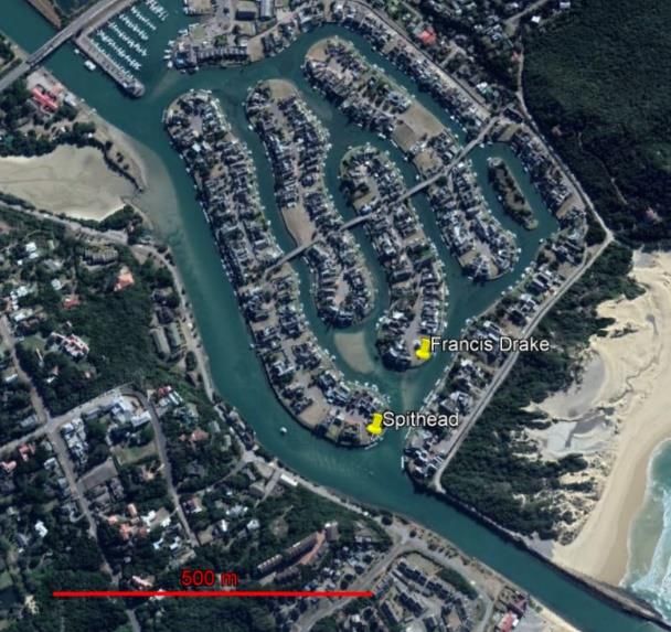
3 Study Sites
Royal Port Alfred Marina (from now on referred to as Port Alfred Marina) was
chosen as the main study site for three major reasons. Its environment
accommodates mussel populations, which was important to secure the
biological component. It is also considered to be a safe environment, since it
limits the hazards involved in the measurement procedures, as compared to
the wave-swept rocky shores. Being in a gated community, it also ensures that
the risk of theft of equipment is minimised. Thirdly, the site incorporates an
almost unidirectional flow along the shoreline walls and thereby eliminates
interfering factors during the measurements. This ensures that the data
would be acquired reliably. Another aspect is that knowledge about the
hydrodynamics in an artificial environment and its correlation with mussel
populations may be of interest for the community in Port Alfred Marina, along
with other similar manmade sites.

Figure 1. The location of Port Alfred on a map of South Africa (coordinates: 33°36'1.56"S,
26°53'47.85"O) (GoogleEarth, n.d.)

 9

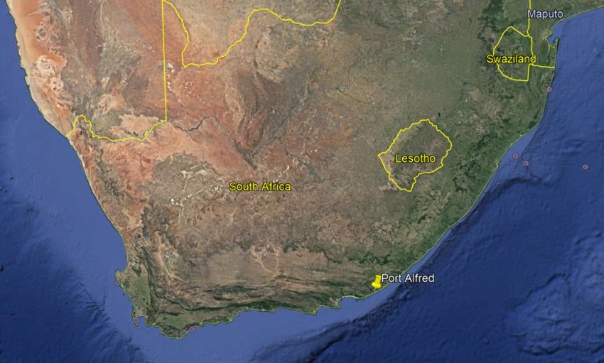
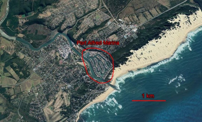
Figure 2. Map showing Port Alfred and its vicinity. Port Alfred Marina is circled in red (coordinates:
33°36'1.56"S, 26°53'47.85"O). (GoogleEarth, n.d.)

3.1 General site information
Port Alfred marina, which is part of the town Port Alfred, makes up part of
the estuary of Kowie river, just before the river outlet meets the ocean (Cock,
2018, pp. 118-119) (figure 1,2). The population of Port Alfred is estimated to
about 65 000 people, of which 25 000 are permanent residents (CMW, 2020;
Cock, 2018, p. 22). The small proportion of permanent residents leads to a
sporadic activity in the area and every year, during December, there is a great
influx of holiday makers in Port Alfred. The boat traffic is then likely to
increase, leading to more turbulent waters. This effect could in turn increase
sedimentation onto the detriment of mussels, as well as interfering with the
normal flow conditions (Thorp & Rogers, 2011). The runoff from the river may
also increase pollution of the waters, which could negatively affect the mussel
populations. The wastewater treatment plant which is dealing with most of
the domestic wastewater in Port Alfred is situated next to the Kowie River,
about 3,6 km northwest of the Kowie river mouth (CMW, 2020). The effluent
of the facility is flowing into the river and eventually reaches the marina. The

 10

treatment plan has in recent years not treated the water at full capacity and
coliform concentration in the water is therefore suggested to have risen
(Cock, 2018, pp. 130-135).

The tidal reach up the river is estimated to be 21 km, while the freshwater
inflow to the river can be considered less than 1 m3/s (Schumann, Gray, &
Shone, 2001). Consequently, the predominantly greatest physical feature
affecting the mixing processes in the marina is deriving from tidal flows. The
amplitude of the tides is ranging from 0,5 m during neap tide to 2 m during
spring tide (Schumann, Gray, & Shone, 2001). At certain instances, the rising
tide brings lines of foam into the marina, near the mouth (Cock, 2018, pp. 23-
24). This feature incorporates the trapping of plankton, such as mussel larvae,
which are caught in the circulation (Cock, 2018, pp. 23-24).

After the construction of the marina 1989, the estuary increased greatly in
circumference (Schumann, Gray, & Shone, 2001). Consequently, the water
motion naturally slows down in some sections of the marina, leading to
increased sedimentation, which could have an effect on the mussel
populations (Schumann, Gray, & Shone, 2001). In order to counter the
continuous build-up of silt deposits, the marina is regularly being dredged
(Cock, 2018, pp. 118-119). The dredging process could however be hazardous
to the marine environment and does also involve using floating pipes, which
are lined out along central areas of the channel sections. These may act as
barriers, blocking part of the natural flow in the marina and interrupting
propagation of matter transported near the surface.

The seasonal variation in the area has an impact on weather and sea condition
and the two-month study is not incorporating this change. The measurements
took place during the late summer months when the conditions generally are
milder. The wave height differs significantly, being greater in winter than
summer (figure 3a). The wind speed follows a similar pattern to that of the
wave height (Wisuki, 2020) and the wind direction is altering over the year,
with south-easterly winds during the study period (Windfinder, 2020). The
rainfall is sporadic over the year, with generally more rain during the time of
measurements (figure 3b). The increased rainfall would likely increase the

 11

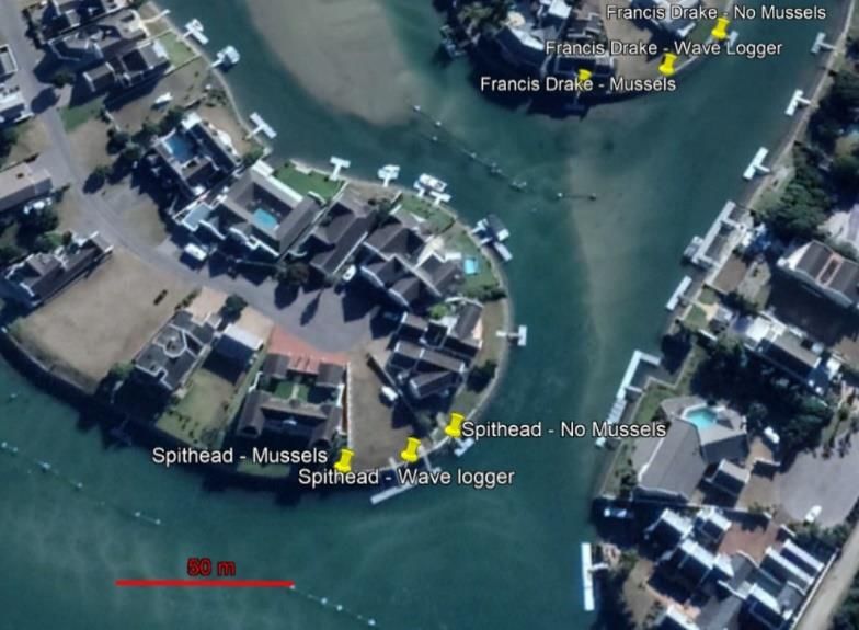
flow in the river, which could have a minor effect on the hydrodynamics and
water quality in the marina.

Figure 3a. Monthly wave size in Port Alfred over the year (Wisuki, Port Alfred, Eastern Cape, South Africa,
2020).

Figure 3b. Monthly Rainfall in Port Alfred over the year (Wisuki, Port Alfred, Eastern Cape, South Africa,
2020)

3.2 Points of measurement
Field measurements were carried out in Port Alfred Marina, although minor
comparable measurements were conducted in Kenton-on-sea. Ethical
clearance for the field surveys related to the project were in place through
SAIAB ethical committee prior to the measurements. Permission to perform
measurements in the gated community “Royal Port Alfred Marina” complex
was also confirmed before each entry.

Within Port Alfred marina, two sites were selected where field measurements
took place, from now on referred to as “Spithead” and “Francis Drake”
(named after the street names adjacent to the sites). Within each site, two
subsites were further selected (figure 5). The subsites were separated by the
presence of mussels and were hence referred to as “mussels” and “no
mussels”. Each subsite stretched about 10 meters along the armouring. Wave
loggers were deployed in between the two subsites on each site (figure 5) and
were thereby representing both subsites within each site. The “mussel” and
“no mussel” subsites were situated approximately 20 meters apart and were
 12

both adjacent to a private jetty, meaning that they shared similar features.
Similarly, both Spithead and Francis Drake were situated close to the mouth,
faced the same direction and presented the same armouring material. The
similar characteristics between the sites hence eliminates unwanted factors
within the experimental design.

 13

Figure 4. The satellite image is presenting both the Spithead site (coordinates:
33°36'1.45"S, 26°53'48.59"O ) and Francis Drake site (coordinates: 33°35'57.14"S, 26°53'51.71"O ) in
Port Alfred (GoogleEarth, n.d.).

Figure 5. The satellite image is presenting the subsites “Spithead mussels” (coordinates: 33°36'1.56"S,
26°53'47.85"O), “Spithead no mussels” (coordinates: 33°36'1.20"S, 26°53'49.07"O), “Francis Drake
mussels” (coordinates: 33°35'57.34"S, 26°53'50.61"O), Francis Drake no mussels (coordinates:
33°35'56.69"S, 26°53'52.41"O), as well as the location of the Spithead wave logger (coordinates:
33°36'1.45"S, 26°53'48.59"O) and the Francis Drake wave logger (coordination:
33°35'57.14"S, 26°53'51.71"O) (GoogleEarth, n.d.)
 14

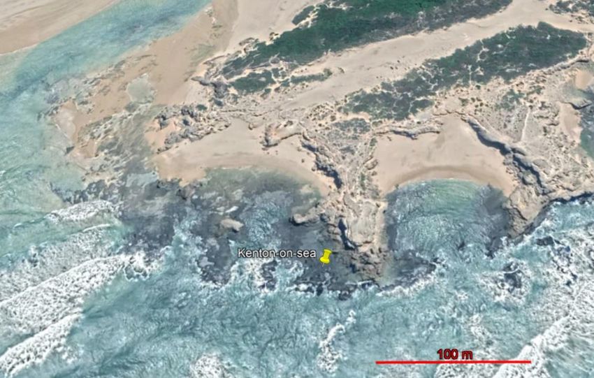
3.3 Kenton-on-sea
Kenton-on-sea was chosen as the rocky shore site, where a wave logger was
deployed to measure hydrodynamic patterns in a natural mussel habitat
(figure 6). The wave height data from this site would then be compared with
measurements in the artificially constructed Port Alfred Marina to see what
the factorial difference was within this variable. The site is characterised by a
rocky shore platform of Aeolian dune rock and exposed to the direct force
from incoming waves. It is situated 23,9 km down the coastline from the Port
Alfred site and the area is thereby experiencing similar sea and weather
conditions (figure 6). Just like Port Alfred, it is also situated at the end of a
river outlet, Bushman’s river.

Figure 6. Map of the ”wild site” Kenton-on-sea (coordinates: 33°41'44.96"S, 26°39'57.95"O)
(GoogleEarth, n.d.)

 15

4 Experimental design of field measurements
The physical and biological measurements are separated within this section.
The most thorough measurements were the recordings of velocity next to the
mussel substrate. Along with these, wave measurements were conducted,
adding further depth to the physical data. Thereafter, measurements of
settlement and identification of mussel larvae are described. Finally, the last
section unfolds how the data was analysed, uniting the physical and biological
measurements. Henceforth, the term “mussels” refers to the species Mytilus
galloprovincialis and/or Perna Perna, unless explicitly stating otherwise.

4.1 Overall design
The exact design of the study is unique and has not been utilised before. The
method can thereby be seen as a combination of many previously used
techniques, combined to enhance novel findings between biological and
physical components. Measurements were taken over a period of 8 weeks,
starting from 26th of January and finishing 19th of March and sampling was
planned to follow trends in neap and spring tide. The data considered to
represent spring tides were sampled during days when the tidal forecast
website, Wisuki (Wisuki, 2020), were predicting the highest tidal heights for
high tides during a two week period. Similarily, the data considered to
represent neap tides were sampled during days when Wisuki was predicting
the lowest tidal heights for high tides during a two-week period.
Measurements covering a certain tidal phase always took place over three
consecutive days. The only week when the days of measurement deviated
from this pattern was when a prompt meeting day at SAIAB was declared due
to the an immediate threat of the novel coronavirus outbreak (Cohen &
Kupferschmidt, 2020) and no field trips were allowed during this day. The
consequence being that the days of measurements were postponed by one
day for the last measured neap tide and were therefore slightly less
representative of this tidal phase.

The substrate of the armoured shoreline consisted of a manmade cobbled
rock wall, which at depth connected with a flatter rocky/silty bottom (figure
9). The slope was measured at the different subsites to establish if this

 16

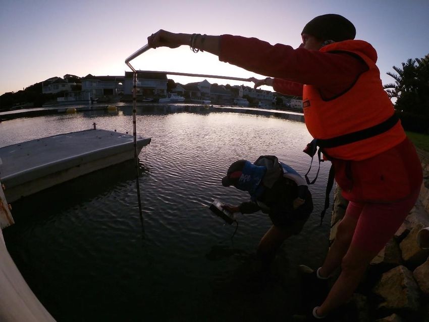
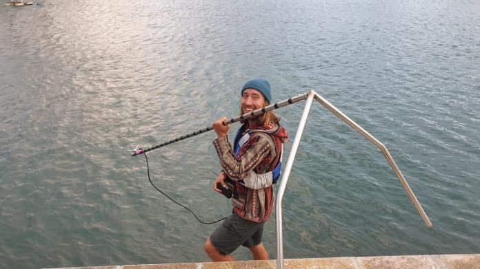
physical feature differed significantly. This was performed by using a
measuring tape during low tide when the shore was dry. The vertical depth
change was then measured as one moved 250 cm horizontally out from shore
(starting from the spring high tide mark).

Physical and biological measurements were conducted equally on the mussel
and the no mussel sites. The main component of the physical variables was
the water velocity. Paired with this, measurements of temperature, depth,
salinity and wave characteristics were sampled. Biological measurements of
larval settlement were also conducted alongside the physical measurements
and as a once off measurement the adult mussel distribution at each subsite
was determined. More in detailed descriptions of the different
measurements incorporated in the study are presented through separate
sections below.

4.1.1 Physical data collection
To characterise the speed and direction of the currents adjacent to the
substrate, an acoustic doppler velocimeter (ADV) was used (SonTek/YSI,
2007). The instrument utilises sound to estimate velocities. The point of
measurement is situated 10 cm horizontally from the probe and the local
velocity could thereby be measured. Other parameters, such as temperature,
spikes and velocity error, were also recorded. In this regard, spikes are likely
to represent dramatic instantaneous changes in velocity (SonTek/YSI, 2007).
Although, bigger particles interfering with the transmitted soundwaves may
also cause spikes (SonTek/YSI, 2007). The velocity error is another parameter
given by the console, which directly describes the accuracy of the velocity
data (SonTek/YSI, 2007). High changes in velocity error are likely caused by
turbulence in the water, which could be of interest when relating the data to
mussel behaviour.

To ensure consistency of measurements, a metal rod was designed on which
the probe could be mounted on. It was made of stainless steel in order to
prevent rust and hollowed in the centre to keep it light and thus make it more
manageable. Two stainless steel “handlebars” were connected to the top of
the rod, making it possible for the person sampling to stand further away from

 17

the point of measurement and keep the metal rod steady (figure8). The
properties of the rod are given in the illustration below (figure 7).

Figure 7. Configuration of ADV mounted on the metal rod during measurements, along with relevant
scales.

Since the handheld console only can withstand being submerged briefly, it
was decided to avoid any submersion whatsoever. It was therefore important
that two people were present during the time of field sampling, one holding
the console and one keeping the metal rod balanced. During measurements,
the rod was weighted on the bottom, which ensured that the ADV readings
were kept stable and minimally interfered with. The length of the metal rod
is limited to the length of the ADV wire, which is 2 meters long and cannot be
prolonged as it is a permanent attachment. Measurements could therefore
never exceed 2 meters depth. This however did not affect the accuracy of the
measurements. In order to keep track of the sampling depth, the metal rod
had labelled markings (every 10 cm) along its length, from bottom to top. By
subtracting the average depth of the submerged part of the rod with the
height of which the ADV probe was mounted on, it was determined on which
depth each measurement took place on. The ADV probe was always secured

 18

10 cm above the bottom of the rod, making the point of measurement equally
distanced (10 cm) vertically as horizontally from the substrate.

Figure 8. Picture demonstrating the technique used when performing velocity measurements with the
Acoustic Doppler Velocimeter.

The local velocity was measured at the sites Spithead and Francis Drake,
including both their respective subsites. Since only one probe was allocated
for this study, the measurements could not be made simultaneously at
subsites/sites. To avoid the influence of delay in time between samples, there
was a continuous alternation between starting sites of measurement.
Consequently, each site served as starting site for the measurements an equal
number of times. From preliminary visual inspections of the sites, it could be
concluded that the mussel populations were fully covered for a period of six
hours per tidal cycle, starting roughly three hours before high tide and
finishing around three hours after high tide. To ensure that the mussels were
submerged in sufficient water (to steadily measure the velocity), the
measurements started 2 hours and 40 minutes before high tide and finished
2 hours and 40 minutes after high tide (table 1). Since the velocity was
 19

fluctuating over time, each measurement was set to either two or three
minutes and thereby the average velocity could be more representative. The
measurements were divided into three separate sets, covering rising, high
and receding tide, as seen in table 1. The velocity measurements during high
tide were set to 2 minutes each, ensuring that the measurements did not
extend beyond the time of the highest tidal stage.

Table 1. Starting time, finish time and time per individual measurement for the separate tidal stages.

 Tidal stage / Rising tide High tide Receding tide
 parameter
 Starting time 2h40min before 30min before 1h after high tide
 high tide high tide
 Finish time 1 hour before 30min after high 2h40min after
 high tide tide high tide
 Time per 3 min 2 min 3 min
 measurement

Measurements at each subsite included velocity recordings near the dense
part of the mussel populations (shallow part), near the deeper more scattered
mussel population and near the jetty (figure 9). To consolidate the data
acquired from the non-jetty measurements, there were always two replicates
for every measurement, while keeping one replicate for the jetty
measurements. The different sections of each subsites were chosen to
determine if there were any patterns regarding the depth. The shallow
measurements were randomly taken within a standard depth where the
denser mussel populations were found. For the “no mussel sites”, the depth
of measurement always mirrored the design of the “mussel sites”. The deeper
section was on average 60 cm deeper than the shallow section and points of
measurement were randomly chosen within this depth. Since the jetty
measurements were situated near the middle of the channel, it was
considered to roughly represent the flow in the middle of the channel. As a
proxy the depth was set to 1,5 m depth at the jetty. Depth relative to the
bottom however changed as the jetty floated up and down with the tidal
movements.

 20

Figure 9. Cross section of the sites of measurement. The cobbled rock wall meets a flatter rocky/silty
bottom. The different sections of measurement are illustrated, shallow, deep and jetty.

Since salinity may affect the velocity measurements and stand as a factor
explaining mussel distribution, it was also measured in between velocity
measurements. From trial measurements it was seen that the salinity did not
change between the subsites, but between the sites. The salinity was
therefore only measured three times per set of measurements at each site.
The salinity was measured with a portable handheld refractometer. The
results of the velocity measurements were stored in the console and
transferred to a computer. Through the corresponding Flowtracker v.2.3
software (SonTek/YSI, 2007), the data was sorted and in turn sent to excel for
further analysis.

4.1.2 Wave measurements
Measurements of wave properties was carried out with wave loggers, which
recorded the hydrostatic pressure over time and translated it into ambient
wave characteristics. The measurements were taken in bursts with a 10 Hz
frequency every hour and lasted for 11 minutes. The batteries of the wave
loggers were constructed to last longer than a month and all the recordings
were saved on an sd-card.

 21

Figure 10. Picture illustrating the configuration of the deployed wave loggers used at the various sites.
The wave logger was secured with cable ties to metal bolts, which in turn were firmly screwed into a 30
kg heavy rock. As an extra security, a rope was attached to the configuration with the other end knotted
around an eye bolt further up the shoreline.

The wave loggers were deployed at the bottom in between the “no mussel”
and “mussel” subsites on Spithead and Francis Drake, respectively. The wave
loggers were secured by attaching them to 30kg heavy rocks with cable ties
(figure 10). Five holes were drilled into each rock, in which eye bolts were
screwed in and attached to the cable ties. The wave loggers were positioned
at a depth and point relative to the wall where the mussels were found on
the “mussel” subsites. In the same fashion wave loggers were deployed in
Kenton-on-sea. There, the instrument was secured in a small rock pool to
minimise stress from the violent wave-swept environment. The instrument
was surrounded by mussel beds and could therefore be seen to represent the
wave characteristics of a natural mussel bed environment. The wave logger
in Kenton-on-sea was situated 24 km from the wave loggers in Port Alfred
(GoogleEarth, n.d.) and could thereby be seen as a local natural habitat near
Port Alfred. Unfortunately, the wave loggers used were faulty and only
sporadic data was obtained over the period of measurements. By uploading

 22

the data to Obscape’s online software (Obscape, 2020), the depth, significant
wave height and wave period could be acquired.

4.2 Biological data collection
4.2.1 Collection of mussel larvae
Combined with the physical measurements in Port Alfred Marina, biological
measurement of temporal and spatial settlement of mussel larvae were
monitored by using artificial collectors (plastic scouring pads) (Porri,
McQuaida, & Radloff, 2006). The main target species were Perna Perna and
Mytilus galloprovincialis, although all collected bivalves were noted.

The settler collectors were tied with plastic cable ties to a 0,5 kg weight, which
in turn was tied to the end of a fishing line. The other end of the fishing line
was firmly secured to a metal peg, which was sunk into the grass on top of
the stone wall of each site (as seen in figure 11). In this way, the settler
collectors were hanging along the wall at a depth where mussels were found,
alternating between being submerged and exposed as the tide moves the
surface level. This deployment technique inferred no permanent scarring of
the marina construction and made it easy to exchange the settler collectors
at any stage of the tide (although, the time of low tide was targeted). Five
scouring pads were deployed at each subsite, approximately two meters
apart. They were exchanged on a weekly basis over a period of 8 weeks. New
settler collectors were routinely deployed at the end of the last day of weekly
flow measurement. Consequently, the scouring pads were tied to a certain
tidal phase, representing settling of mussel larvae either during spring tide or
neap tide. When the settler collectors were taken out, they were
independently put into 250 ml sealable plastic jars and fully covered with 90%
ethanol as preservative. Since the plastic cable ties could be holding larvae as
well, these were also put in the jars together with the collectors.

 23

Figure 11. Cross section of the sites of measurement. The cobbled rock wall meets a flatter rocky/silty
bottom. The anchoring metal peg is holding one end of a fishing line, which is attached to a scouring
pad on the other end (which larvae may settle on).

4.2.2 Processing of settler collectors
Three of the five sample jars containing scouring pads and cable ties from
each site were processed. In the case of a lost settler collector or other
factors, there would in this way always be two extra scouring pads for
analysis. Before the samples could be analysed, the collected matter had to
be removed from the scouring pads and cable ties. In the laboratory at SAIAB,
5ml of bleach (sodium hypochlorite) was pipetted into each plastic jar and
after being well shaken they were left to soak for 5 minutes. This procedure
ensured that the cemented byssal threads of the collected mussels were
adequately dissolved, making them easier to remove from the scouring pads
(Davies, 1974). The content of each jar was then poured over a 75μm sieve,
blocking thicker solid matter (potential mussel collectors). By then cutting and
unravelling the scouring pads, it was then possible rinse of the remainder of
solid matter over a 10L bucket. When all the matter from both the scouring
pad and the cable ties had been removed, the content of the 10L bucket was
poured over the 75μm sieve. The solid matter in the sieve was then flushed
into a plastic jar along with 20 ml of 90 % preserving ethanol and the samples
were thereby ready for the identification process.

 24

4.2.3 Identification of mussel larvae
Each sample was examined by the use of a Leica MZ75 stereoscopic dissecting
microscope. By adding the content of each processed samples into petri
dishes, it was possible to systematically inspect the content and look for
larvae of bivalves, mainly Perna Perna and Mytilus galloprovincialis.
Identification of the specimens was made according to the key morphological
traits (Bownes, Barker, & McQuaid, 2008). The mussels were also
distinguished by size, where the smaller specimens (360μm) were classified as “recruits”
(Porri, McQuaida, & Radloff, 2006). Identified mussel specimens were finally
collected in enclosed Eppendorf tubes where they were preserved in 90%
ethanol. Conclusively, the species, number of specimens and size class were
noted.

4.2.4 Distribution of adult mussels
Abundance of adult mussels was determined by a once-off census of their
percentage coverage at the different subsites. These measurements were
performed at the very start of the study, to prove the difference in mussel
existence between the “mussel” and “no mussel” subsites. The distribution
and abundance of adult mussels (of the species Perna Perna and Mytilus
galloprovincialis) were determined by combining the quadrat and line
intercept transect sampling methods (Montaggioni & Braithwaite, 2009, s.
20). An 11 meter transect line was laid out along a depth where the densest
adult mussel population was observed, being in line with where the shallow
velocity measurements were being conducted and where the scouring pads
were deployed. Quadrats of the size 55x55cm were then laid out on each side
of the transect line as figure 12 illustrates. One side of the quadrat always
followed the transect line and a total of 20 quadrats were used, making up
the entire 11 m length of the transect line. Each quadrat was made up of a
grid with 100 intersections. The quadrats were inspected visually and the
number of intersections per grid that covered a mussel was counted, serving
as one percent each. The percentage of mussel coverage per quadrat was
thereby estimated for all 20 quadrats along each transect line. Consequently,
the average mussel coverage of 20 quadrats represented the density of
mussels on each subsite. Due to the imminent corona virus outbreak, the last
field trips from SAIAB were cancelled and there were no possibility to

 25

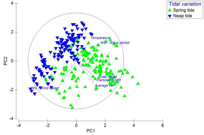
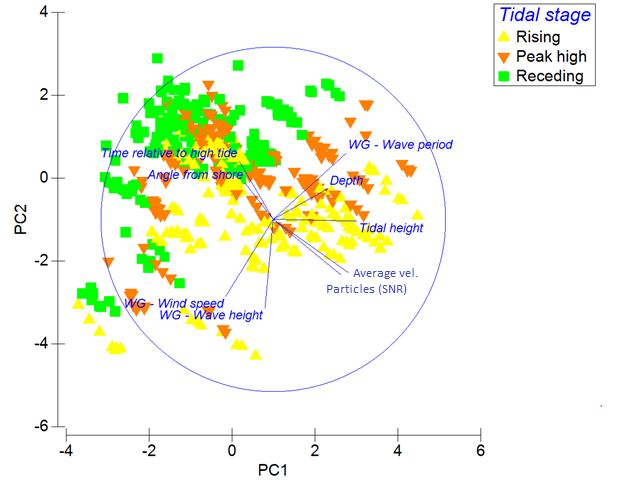
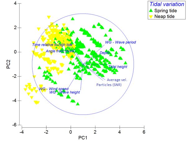
measure the mussel coverage on the Kenton-on-sea site (Cohen &
Kupferschmidt, 2020).

Figure 12. Distribution measurements represented by quadrats in blue and transect line in red.

5 Data Analysis
The data was first refined before being analysed through either excel or
PRIMER v6.1.15 with PERMANOVA+ (Anderson, Gorley, & Clarke, 2020). Since
the main element of the study was the measured flow velocities, the data was
analysed in a fashion that focuses on the effect of the average velocity in
relation to the rest of the data. In order to highlight different trends, the
procedures described in this section were repeated for separate subsets of
the data. The subsets of data incorporated are presented in table 2 below.

 Subsets of data used in separate data analysis procedures
 Only data related to the shallow measurements
 Only data related to the deep measurements
 Only data related to the jetty measurements.
 Only data related to the shallow and deeper measurements
 Only data from when the significant wave height was measured (only
 shallow velocity measurements)
 Only data from the 24 hour period when the night measurements were
 conducted
 All data
Table 2. Subsets of data used in separate statistical analysis.

The vast majority of the larval samples did not contain any mussels. The data
thereby contain too many “zeros” to be included in any adequate statistical
analysis and the biological dataset was unfortunately removed from further
analysis.

5.1 Data included in the analysis
Parameters classified as part of the “environmental data” are either based on
in-situ measurements or recovered from online sources (table 3).
 26

Table 3. Parameters included in the statistical analysis along with their units.* The jetty velocity
parameter is excluded when the jetty measurements are included in the specific subset of data analysed.
** The significant wave height is only included when looking at the subset of data which specifically
focuses on the parameter.

 Parameter Unit Parameter Unit
 included included
 Average velocity [m/s] Time [hh:mm]
 Max velocity [m/s] High tide time [hh:mm]
 Average velocity [m/s] Time relative to [hh:mm]
 error high tide
 Jetty velocity* [m/s] Spikes N/A
 Angle from shore [degrees] Wakes reported N/A
 Particles (SNR) N/A WG – Windspeed [knots/hour]
 Salinity [‰] WG - Wave height [m]
 Depth [cm] WG – Wave [s]
 Tidal height [cm] period [%]
 Tidal constant N/A Adult mussel [m]
 Date [Day from coverage
 start] Significant wave
 height**

The “average velocity”, “max velocity” and “average velocity error” were all
given one value per measurement and were calculated through an excel
spreadsheet. When subsets of data were used which did not include jetty
measurements, the “jetty velocity” parameter could be seen as a proxy for
the flow closer to the midsection of the channel. “Angle from shore”
represents the angle in which the flow direction flowed relative to the
shoreline. The average amount of particles present per measurement is
included in the “particles (SNR)” variable and denotes both dissolved and
suspended particles. The “salinity” represents an average value of three
measurements per site. The “depth” relates to the actual depth where the
velocity was being measured. The “high tide time”, “tidal height” and “tidal
constant” was extracted from an online source (Wisuki, 2020) and has one
value per day of measurements. In addition to the tidal height, the tidal
constant also takes into consideration the time in between tidal stages. The
 27