Unsupervised Doppler Radar Based Activity Recognition for e-Healthcare
←
→
Page content transcription
If your browser does not render page correctly, please read the page content below

SPECIAL SECTION ON BEHAVIORAL BIOMETRICS FOR EHEALTH AND WELL-BEING

Received March 18, 2021, accepted April 7, 2021, date of publication April 19, 2021, date of current version April 30, 2021.
Digital Object Identifier 10.1109/ACCESS.2021.3074088

Unsupervised Doppler Radar Based Activity
Recognition for e-Healthcare
YORDANKA KARAYANEVA 1 , SARA SHARIFZADEH1 , WENDA LI 2 ,
YANGUO JING1 , (Member, IEEE), AND BO TAN 3 , (Member, IEEE)
1 Faculty of Engineering, Environment and Computing, Coventry University, Coventry CV1 2JH, U.K.
2 Department   of Security and Crime Science, University College London, London WC1E 6BT, U.K.
3 Faculty of Informaon Technology and Communicaon Sciences, Tampere University, 33100 Tampere, Finland

Corresponding author: Bo Tan (bo.tan@tuni.fi)

  ABSTRACT Passive radio frequency (RF) sensing and monitoring of human daily activities in elderly
  care homes is an emerging topic. Micro-Doppler radars are an appealing solution considering their non-
  intrusiveness, deep penetration, and high-distance range. Unsupervised activity recognition using Doppler
  radar data has not received attention, in spite of its importance in case of unlabelled or poorly labelled
  activities in real scenarios. This study proposes two unsupervised feature extraction methods for the purpose
  of human activity monitoring using Doppler-streams. These include a local Discrete Cosine Transform
  (DCT)-based feature extraction method and a local entropy-based feature extraction method. In addition,
  a novel application of Convolutional Variational Autoencoder (CVAE) feature extraction is employed for
  the first time for Doppler radar data. The three feature extraction architectures are compared with the previ-
  ously used Convolutional Autoencoder (CAE) and linear feature extraction based on Principal Component
  Analysis (PCA) and 2DPCA. Unsupervised clustering is performed using K-Means and K-Medoids. The
  results show the superiority of DCT-based method, entropy-based method, and CVAE features compared to
  CAE, PCA, and 2DPCA, with more than 5%-20% average accuracy. In regards to computation time, the two
  proposed methods are noticeably much faster than the existing CVAE. Furthermore, for high-dimensional
  data visualisation, three manifold learning techniques are considered. The methods are compared for the
  projection of raw data as well as the encoded CVAE features. All three methods show an improved
  visualisation ability when applied to the encoded CVAE features.

  INDEX TERMS Activity recognition, data visualization, Doppler radar, health and safety, DCT analysis,
  unsupervised learning.

I. INTRODUCTION                                                                                   The demand for human activity detection and monitor-
Human activity recognition for smart healthcare is an emerg-                                   ing has rapidly increased over the past years. A number
ing topic. It is becoming even more prominent with the com-                                    of devices are proposed including cameras, wearable tech-
plications of ageing population worldwide. The population                                      nologies, infrared sensors, and radars. These devices are
aged 65+ in the UK was 11.8 million in 2016, while this                                        expected to provide daily monitoring of elderly people’s
number is projected to grow to 20.4 million by 2041 [1].                                       activities and vital signs. Hence, this will provide peace of
Chronic and long-term conditions are well-known to increase                                    mind for their relatives regarding the physical health and
with age. It is reported that 29% of those aged 60-64 had a                                    mental health of the care home residents. Cameras are often
chronic condition, while the percentage grows to 50% for                                       seen as an obvious and traditional solution for capturing
elderly populations aged 75 or over. The implications of                                       observable data including human activities for subsequent
ageing with chronic conditions prevent elderly people from                                     recognition [2]–[4]. Video-depth cameras are capable of
independent living. Thus, they are dependent on social care                                    obtaining extremely high-resolution data, which can con-
services such as living in care homes.                                                         tribute to the detailed analysis of daily human activities. Nev-
                                                                                               ertheless, camera devices suffer from intrusiveness, which is
    The associate editor coordinating the review of this manuscript and                        highly undesirable in the contexts of residential environment.
approving it for publication was Donato Impedovo              .                                The modern healthcare is concerned with the privacy and

                     This work is licensed under a Creative Commons Attribution 4.0 License. For more information, see https://creativecommons.org/licenses/by/4.0/
62984                                                                                                                                                                 VOLUME 9, 2021
Y. Karayaneva et al.: Unsupervised Doppler Radar Based Activity Recognition for e-Healthcare

dignity of patients. Therefore, vision-based solutions are not                     standard PCA for Doppler radar data [28]. Considering the
recommended in smart care homes.                                                   fact that 2DPCA accepts 2D image matrices as an input,
   Wearable sensor technologies are an effective solution for                      the dependencies of the pixels are retained. The results of
smart healthcare applications as they provide a combina-                           that work revealed improved recognition rates for 2DPCA
tion of human activity recognition and vital signs detection                       by more than 10%. Furthermore, unsupervised PCA has
[5]–[8]. Wearable sensors have the ability to capture small                        been combined with supervised Linear Discriminant Anal-
fractions of the body such as the movement of fingers [9].                         ysis (LDA) and shallow neural networks (SNN) [29]. The
Additionally, wearable sensing technologies can detect phys-                       proposed architecture in that work was the first to use a
iological signals such as heart rate and speech patterns [10].                     3D-signal representation by retaining the matrix dependen-
However, the disadvantages and challenges of this technology                       cies. Results reveal better performance than conventional
are not to be under-rated. Wearable sensors are known to                           PCA and 2DPCA for Doppler radar data.
have poor battery life [11]. As they are ‘‘wearable’’, elderly                        In a pilot study, the Doppler-Radar-2018 dataset was
populations may easily forget to wear the device or feel                           used. The work employed Hidden Markov Models (HMM)
uncomfortable wearing it [12].                                                     in order to extract activity information from each Doppler
   Infrared sensors utilize human’s body temperature dis-                          sequence [23]. The output of the HMM training was clus-
tinguished from the lower ambient temperature in order to                          tered using K-Means and K-Medoids. The Kullback-Leibler
capture and detect human activities. Most IR sensors obtain                        (KL) log-likelihood with K-Medoids for clustering obtained
ultra low-resolution data, where a subject identification is                       the highest accuracy. HMM is a supervised framework that
avoided. Thus, IR devices represent an attractive solution                         requires the labels and generates log-likelihood values as
to be deployed in care homes and hospitals. Current stud-                          a measure of similarity of a candidate sample to each of
ies reveal significant recognition rates (>90%) for activi-                        the classes. Therefore, log-likelihood values can be used for
ties including standing, sitting, walking, falling, and others                     decision making directly and the idea of using them as a
[13]–[15]. Contrarily to their advantages, IR devices suffer                       feature and applying unsupervised methods such as K-Means
from a relatively low detection distance. It can be inferred                       for clustering them is not the best analysis pipeline. HMM
in a recent dataset [16] that the performance drops with                           was also used in another previous work [30], for classifica-
distance growth, although not significantly. As IR sensors                         tion of extracted physical features where 72% accuracy was
are low-resolution capturing devices, they lack sensitivity                        achieved.
towards small fractions of the human body, which prevents                             Another group of supervised techniques are based on
more specific activities detection.                                                deep learning approaches. These methods require more data
   Passive Micro-Doppler radars are an appealing solu-                             for learning their objective functions. Recently, Convolu-
tion for human activity recognition. That is due to their                          tional Neural Networks (CNNs) and Recurrent Neural Net-
non-intrusiveness, high distance range, deep penetration, and                      works (RNNs) architectures have been used. Furthermore,
reliable accuracy rates [17]–[19]. In addition, the passive                        CAE was used for feature extraction for Doppler radar data
radar uses the existing radio bursts in the environment.                           [31]. That was followed by classification based on a super-
It avoids to bring extra RF source to aggravate the increasing                     vised framework by fine-tuning and a Softmax classifier.
electromagnetic interference in the residential environment.                       In these techniques, feature extraction from data streams
While passive Micro-Doppler radars traditionally have appli-                       are performed automatically with minimum user required
cations in human activity recognition [17], they have also                         settings [32].
been deployed for vitals sign monitoring such as respiration                          Unsupervised learning is yet a minimally researched topic
[20]. In addition to their applications, the devices have been                     for Doppler radar based applications. The advantage of unsu-
used for gait patterns analysis [21].                                              pervised methods compared to supervised techniques is that
   Micro-Doppler radars have been extensively used for activ-                      they do not require labeling data. This usually influences
ity recognition with a focus on healthcare purposes [20], [23],                    the accuracy of unsupervised methods compared to super-
[24]. Currently, majority of studies are based on pipelines,                       vised techniques. That is because in the absence of labels,
which are totally supervised or consist of a combination                           the learning is only guided based on the input variables, their
of unsupervised and supervised approaches. In most cases,                          variations and characteristics. That does not necessarily help
the pipelines are based on unsupervised feature extraction                         to learn the decision rules correctly. However, the models
methods, such as conventional PCA and Singular Value                               can be updated faster compared to the supervised strategies.
Decomposition (SVD) techniques. That is usually followed                           Hence, the learning capacity of the latter are limited due to
by a supervised classification method, such as Support Vec-                        labeling requirement for any new coming data. In practi-
tor Machine (SVM) and k-Nearest Neighbours (k-NN) [25],                            cal settings, usually recognition of few activities is critical
[26]. In the pursuit of a more accurately measured covariance                      such as a fall or immobility. In future, such activities can
matrix from PCA, variations of PCA have been used for                              be labelled and recognized among the clustered activities.
Micro-Doppler data. In [27], the authors applied L1 norm                           However, this work is only focused on unsupervised activ-
PCA opposed to standard PCA and achieved improved testing                          ity clustering of Doppler radar data and the latter prob-
accuracies. Furthermore, 2DPCA has been compared with                              lem is not addressed in this paper. It will be considered

VOLUME 9, 2021                                                                                                                              62985
Y. Karayaneva et al.: Unsupervised Doppler Radar Based Activity Recognition for e-Healthcare

for future studies. In addition, unsupervised learning usually                information, two local patching and feature extraction
requires the use of techniques for estimating the number of                   methods are proposed in this paper. To retain the unsu-
clusters. This is due to the fact that subjects conduct a broad               pervised scenario and evaluate the features, the Dunn’s
number of activities in a real world scenario. As such, embed-                index is used. It is used as a criterion for evaluation of
ding all activities in a pre-collected dataset for supervised                 the activity clustering results, using the locally extracted
frameworks is problematic.                                                    features. That also helped to choose the first proposed
   Unsupervised learning methods can be categorised into                      feature extraction method’s parameters such as the local
two groups of manual or automated feature extraction strate-                  patch size and location. The first proposed method uses
gies. In rule-based systems, specially those strategies based                 2D DCT to extract features from local patches of the
on hand-crafted features, prior knowledge about the experi-                   2D images. The second proposed method is based on
mental system and environment are important [33]. Besides                     entropy of the local patches. The average testing results
that, careful selection of the feature extraction technique                   showcase 5%-10% improvement by using the proposed
and manual selection of some parameters depending on the                      techniques for different scenarios compared to the pre-
setup rules are required. For example, the signal strength and                vious methods. To the best of our knowledge, such
angle of measurement can influence filtering window size                      unsupervised algorithms have not been used for human
and scaling or choice of basis function in spatio-temporal                    activity recognition using Doppler radar data.
feature extraction techniques. On the other hand, in auto-                •   Comprehensive study of unsupervised learning for
mated feature extraction approaches such as CAEs, such prior                  Doppler radar data: This work is a pioneering study
settings are not required. The embedded objective function                    concerning unsupervised learning for Doppler radar
and optimization removes the need for manual settings [34],                   data. Based on a comprehensive study, four different
[35]. Nevertheless, the computational time for automated                      metrics are used to estimate the number of clusters in
feature extraction approaches is more expensive compared to                   the unsupervised framework. That is useful in real sce-
manual feature extraction.                                                    narios, where the number of activities can be high and
   In this paper, the Doppler-Radar-2018 dataset, that                        recognizing few of them among all clustered activities
was used previously in [23], is considered. An                                is required. Additionally in this paper, four groups of
unsupervised framework is developed despite labels avail-                     unsupervised feature extraction strategies are compared:
ability. As explained earlier, the importance of the designed                 the proposed methods based on (1) local 2D DCT and
framework is the applicability to projects with poor labeling                 (2) local entropy are compared by (3) architectures using
scenarios. For this aim, four groups of unsupervised feature                  deep CVAE and CAE, where the former has not been
extraction strategies are considered: (1) frequency-domain                    used previously for Doppler radar data, and (4) previous
analysis based on 2D DCT (2) entropy analysis (3) convolu-                    methods using PCA and 2DPCA. The extracted features
tional filtering strategies based on CVAE and CAE (4) unsu-                   are clustered with K-Means and K-Medoids. The pro-
pervised PCA analysis including 1D and 2D analysis. For                       posed methods based on local DCT and local entropy,
DCT and entropy feature extraction methods, two methods                       and CVAE achieved around 5%-20% higher average
are proposed. The extracted features are clustered into differ-               testing accuracy in comparison with CAE, PCA, and
ent activity groups based on unsupervised clustering strate-                  2DPCA. The proposed methods for feature extraction
gies using K-Means and K-Medoids. In order to evaluate the                    along with CVAE encoded features can be useful for
results, the known labels are utilised only at the result evalu-              unsupervised cases or semi-supervised cases with poor
ation step. Leave-one-subject-out cross validation (LOOCV)                    labeling.
is used so that, the built models are tested on unseen data               •   High-dimensional data visualisation enhancement:
of one subject. Due to the fact that in unlabelled conditions                 Manifold learning methods for high-dimensional data
the number of classes is unknown, four unsupervised metrics,                  visualisation are considered in this study. Doppler radar
namely Elbow, Silhouette, Davies-Bouldin and Dunn’s index                     dataset can benefit in regards to activities data visu-
are used.                                                                     alisation. This can reveal similarities between certain
   The contributions of the study to the research community                   activity groups. The manifold learning methods are
are the following:                                                            known to provide good separation between the classes
   • Two proposed unsupervised feature extraction meth-                       [36]. In this study, CVAE encoded data have been
      ods for Doppler radar data: The Doppler radar data in                   used for data visualisation improvement. For the first
      this study has high dimensionality. When reshaped into                  time for Doppler radar data, in this research the mani-
      2D maps, there are different distinguished patterns for                 fold learning methods’ performance over raw data and
      each activity. On the other hand, the high dimensionality               encoded data using CVAE is employed to illustrate
      leads to an ill-posed problem and over-fitting. Therefore,              any improvement for the sake of visualisation. The
      feature extraction from 2D image maps is employed.                      three methods for high-dimensional data visualisation
      For this aim, the local areas with low level of variation               t-Distributed Stochastic Neighbour Embedding (t-SNE),
      and insignificant information can be cancelled out from                 Multidimensional Scaling (MDS) and Locally Linear
      the analysis. In order to extract the most meaningful                   Embedding (LLE) are compared in the two scenarios.

62986                                                                                                                                VOLUME 9, 2021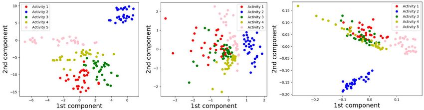
Y. Karayaneva et al.: Unsupervised Doppler Radar Based Activity Recognition for e-Healthcare

      Initially, the methods are used to transform the raw data
      Dn×6400 to a 2-dimensional space. Secondly, the trans-
      formation is performed on the encoded features by
      CVAE data Dn×50 . Comparison of the results reveal
      better separations of the clusters using the three meth-
      ods, when CVAE encoding is used. This showcases the
      strength of CVAE for data separation. Hence, CVAE
      encoded features can be used in manifold learning for
      visualisation purposes.
The rest of the paper is organized as follows: In Section II
the methods including the database description, number of
clusters estimation and the proposed approaches for feature
extraction and clustering are described. Additionally, three
methods for data visualisation are defined. The results for
unsupervised feature extraction and clustering are shown in
Section III. Then, data visualisation techniques are com-
pared by transforming the raw data as well as the CVAE
encoded data. Section IV critically evaluates the main find-
ings of the study, including the proposed architectures for
unsupervised learning and the manifold learning methods
for high-dimensional data visualisation. Finally, Section V
concludes the study with the most valuable outcomes.                               FIGURE 1. Flowchart, describing the overall analysis framework of the
                                                                                   paper.

II. METHODOLOGY
The unsupervised framework in this study consists of a num-
ber of steps as illustrated in Fig. 1. The first step is to divide
data into train and test. Five different activities are recorded
by Doppler radar. The number of clusters K is estimated
using four metrics. Since the raw data are in high-dimension,
unsupervised feature extraction methods are employed to
reduce the feature space dimension. The feature extraction
is followed by clustering and recognition using K-Means
and K-Medoids. Comparison of the proposed two methods
for feature extraction - local DCT-based method and local
entropy-based method is performed with conventional meth-
ods based on CVAE, CAE, PCA, and 2DPCA. The existing
CVAE method has not been deployed in previous Doppler
radar studies.
                                                                                   FIGURE 2. Experimental layout.

A. DATASET DESCRIPTION
The Doppler-spectogram dataset is collected in the University                      spectrogram. More details can be found in Section 3 in [20]
of Bristol laboratory. The laboratory experiment layout is                         or Section III in [23].
shown in Fig. 2 (a 7 m × 5 m room). The radio source                                  Four participants (one female and three male) volunteered
used in this experiment is an Energy Harvesting transmitter                        for capturing activities. This dataset consists of five activities:
(TX91501 POWERCASTER) working on 915 MHz ISM                                       (1) walking, (2) running, (3) jumping, (4) turning, and (5)
band with 30 dBm DSSS signal. The passive radar is a                               standing. Each activity is repeated 10 times by each subject.
two-channel software defined radio (SDR), which is built                           There exist 40 samples for each activity or 200 samples
on two synchronized NI USRP 2920s. Both channels are                               totally.
connected with directional antennas. The reference channel                            A pre-processed Doppler radar dataset is used in this study.
is 1 m apart from the transmitter, while the surveillance                          The total number of features per sample is 6400 = (2 direc-
channel is pointed to the subject. The Cross-Ambiguity Func-                       tions × 100 Doppler bins × 32 time index). Furthermore, the
tion (CAF) which is the Fourier of cross-correlated reference                      Doppler radar data is normalized, which corresponds to the
and surveillance signals is used to 2D range-Doppler plot.                         fact that all features are represented by real values in the range
From each range-Doppler plot, the range column which con-                          of (0, 1). Considering the 3-dimensionality of the Doppler
tains the detected subject is extracted to form up the Doppler                     radar data, it is then vectorized 2 × 100 × 32, which results

VOLUME 9, 2021                                                                                                                                       62987
Y. Karayaneva et al.: Unsupervised Doppler Radar Based Activity Recognition for e-Healthcare

FIGURE 3. Example of an 80 × 80 = 6400 image for each activity: (1) walking, (2) running, (3) jumping, (4) turning, and (5) standing.

in 6400. In order to transform it to 2D maps, 80×80 reshaping
is applied. The reason for converting the vectorized Doppler
radar data into 2D maps, is to apply image analysis strategies
for quantification of local variation and patterns in the image.
Fig. 3 is the micro Doppler signature for human activities.
   The Python libraries used for data pre-processing are pan-
das (version 1.0.5) and numpy (version 1.19.1). In terms
of machine learning for feature extraction and clustering,
scikit-learn (version 0.22.2) and scikit-learn-extra (version
0.1.0b2) modules are applied. The CAE and CVAE are imple-
mented and run with Keras (version 2.2.4) and Tensorflow
(version 2.2.0). The visualisation results are implemented
with matplotlib (version 3.2.2).
                                                                                FIGURE 4. An Elbow test used to determine the number of clusters K .
B. NUMBER OF CLASSES ESTIMATION
Considering the unsupervised scenario in this study, the num-                   decline when the curve approaches the actual K . Therefore,
ber of classes/clusters is unknown. In order to estimate the                    the decline becomes smoother after exceeding K . Fig. 4
correct number, a number of techniques are applied including                    illustrates the Elbow test for this data.
Elbow method, Silhouette analysis, Davies-Bouldin score                            As it can be observed, the selected number of clusters
and Dunn’s index using K-Means clustering.                                      K = 5, which is the actual number of clusters for this study.
                                                                                However, detection of this bend point is ambiguous in some
1) ELBOW METHOD
                                                                                cases. Therefore, additional techniques are considered in this
The Elbow method is a heuristic technique for clusters num-                     study.
ber estimation [37], [38]. The overall goal for the method
is to maximize the inter-class variability and minimize the                     2) SILHOUETTE ANALYSIS
intra-class variability. In this study, the data samples are                    Silhouette analysis is one of the most commonly used tech-
denoted as D = D1 , D2 , . . . , Dn. The number of clus-                        niques for number of clusters estimation [39]. The method is
ters is K and their centroids are given by ω1 , ω2 , . . . , ωK .               given as:
The distortion J is used to measure the effectiveness of the
method:                                                                                                           n
                                                                                                              1 X b(Di ) − a(Di )
                             n
                          1X K                                                               Silhouette =                                                (2)
             J (K , ω) =        (min(Di − ωj )2 )             (1)                                             n  max{a(Di ), b(Di )}
                                                                                                                 i=1
                          n      j=1
                                i=1
In this study, the candidate numbers of clusters K =                            where a(Di ) is the average distance between data point Di and
2, 3, . . . , 10 are selected for K-Means clustering, which is                  the remaining data points in its own cluster. The minimum
described later in this section. The Elbow method computes                      average distance between data point Di and all other clusters
the sum of squared errors for the data samples in each cluster.                 is denoted with b(Di ). The Silhouette coefficient aims to show
As the number of clusters increases, J becomes smaller. How-                    the suitability for data point Di to belong to a particular
ever, the best value of J is the point, where a further increase                cluster. The score is within the range of (−1, 1), where a
to the number of clusters does not change the within-cluster                    lower value refers to overlapping clusters. On the other hand,
sum of squares significantly. However, a further increase                       a higher value suggests well-separated clusters.
would result in over-clustering. The decrease trend of J
is noticeable before reaching the actual number of clusters                     3) DAVIES-BOULDIN INDEX
K and becomes smoother afterwards. The Elbow method                             The Davies-Bouldin index is a clusters estimation method
is a visualisation tool, and the graph shows a noticeable                       concerned with identifying clusters, which are distinct from

62988                                                                                                                                         VOLUME 9, 2021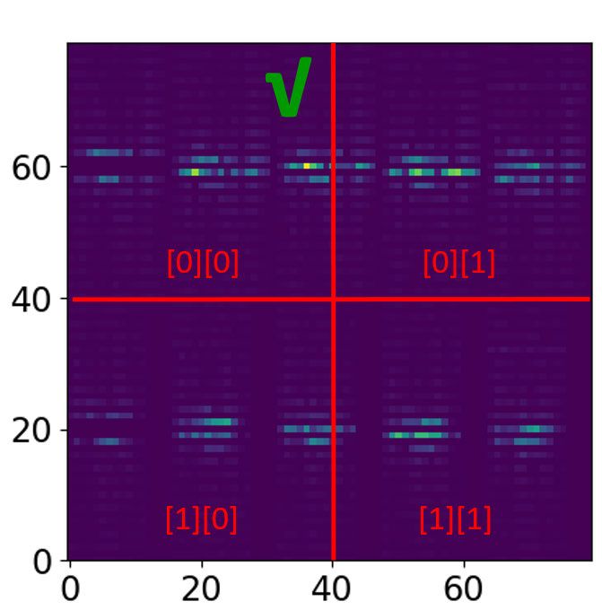
Y. Karayaneva et al.: Unsupervised Doppler Radar Based Activity Recognition for e-Healthcare

each other [40]. The measure is given by:
                            K
                          1 X      1(Ci ) + 1(Cj )
             Davies =         max                                        (3)
                          K   i6=j   λ(ωi , ωj )
                                i=1
                         n
where 1(Ci ) =                  ||Di − ωi ||2 , which is the distance
                         P
                       Di ∈Ci
between each Doppler sequence and the centroid of the cor-
responding cluster. The distance between cluster centroids
is given by λ(ωi , ωj ) = ||ωi − ωj ||2 . Then, the term for
maximization is computing the ratio of within-cluster to
between-cluster distances for the ith and the jth clusters. This
is computed for all combinations of cluster i and other clus-
ters. Then, the maximum value is found for each i. Among
all combinations of clusters, the closest clusters with largest
spreads have the maximum ratio. That is the worst scenario.                        FIGURE 5. Silhouette score, Davies score and Dunn’s index used to
                                                                                   determine the number of clusters K .
The desire is to minimize the overall average of the worst
scenario ratios. Therefore, unlike previous methods, a smaller                     the datasets with uncontrolled or unknown conditions.
value for Davies index is desirable.                                               Later on, the data-driven micro-Doppler recognition
4) DUNN’s INDEX                                                                    approaches are proposed and proven excellent performance in
Dunn’s index is one of the most popular and oldest techniques                      [43]–[45]. These approaches treat the micro-Doppler plots
in the literature [41] for number of clusters estimation. The                      as time-spectrogram and range-Doppler time points clus-
overall aim is to minimize the intra-cluster distance and                          ter respectively. In this work, we will explore two new
maximize the inter-cluster distance. It is given by:                               local DCT-based and local entropy-based methods as well
                                                                                   as convolutional filter-based and variation-based projection
                             min λ(ωi , ωj )
                           1≤i
Y. Karayaneva et al.: Unsupervised Doppler Radar Based Activity Recognition for e-Healthcare

 FIGURE 6. Flowchart of the proposed local DCT-based method.

where, F[p, q] values are the DCT coefficients at row p and
column q. In addition, f [i, j] is the element in row i and
column j of the image matrix, where u = 80 and v = 80,
and 0 ≤ p ≤ u − 1 and 0 ≤ q ≤ v − 1. Moreover, ap = √1 if
                                                                   2
p = 0 and it is 1 otherwise. Similarly, aq = √1 if q = 0 and
                                                   2
its value is 1 otherwise.
   Considering the local variations of the original 80 × 80
images, in this paper, a systematic search algorithm is pro-                  FIGURE 7. The three patching strategies for entropy analysis.
posed in order to find the best strategy for applying 2D DCT.
                                                                              [48] as follows:
This includes applying DCT on different local areas of the
                                                                                                                  b
80 × 80 2D maps, using various patch sizes. The aim is to                                                         X
identify the optimum patch size giving the best clustering                                          H (ρ) = −           ρi log(ρi )                    (6)
results. As illustrated in Fig. 6, first the 2D images are divided                                                i=1

into various square shape local patches of different sizes. The               where ρi is the normalized histogram counts. It is calculated
square-sized local patches are non-overlapping. Four sizes of                 based on the histogram of the image. b is the total number of
local patches are considered - 10×10, 20×20, 40×40 and the                    histogram bins.
original 80 × 80 2D map. Second, each patch is divided into                      Depending on the variations of colors in local image area,
3 × 3 sub-patches. Third, 2D DCT is applied to each local                     the entropy can change. If most pixels in an image are similar
sub-patch and the resulting 2D map of the DC coefficient’s                    with a low level of variations, the entropy will be small.
amplitude is used for feature selection. Third, six coefficients              On the other hand, if the level of color variation is high in
are extracted according to a zig-zag pattern from the top-left                an image, the entropy increases. Therefore, depending on
corner of each sub-patch, allowing to extract features from all               the location of the analysis window, the entropy value can
local areas of the Doppler profiles. Finally, the six features                change. Since the patterns and color intensities vary for differ-
from each of the nine sub-patches are concatenated to form                    ent activities, a careful selection of local patches can generate
a feature vector of size 9 × 6 = 54. This generates 54                        different entropy values suitable for discrimination of the
features for each local patch. Then, the activities are clustered             activities. Based on the observed changes in Fig. 3, three
using the 54 features of each patch and the Dunn’s index                      patching strategies are considered so that, the selected image
is computed. The highest Dunn’s index discovers the most                      areas for entropy analysis are narrowed down systematically.
optimum local patch for the 2D DCT analysis.                                  The three local patchings strategies are illustrated in Fig. 7.
   The reason for using the Dunn’s index in this algorithm is                 Then, similar to the local DCT-based analysis, the Dunn’s
that it describes the quality of the resulting clusters. It quanti-           index is used to evaluate the quality of the clustering results
fies an easily interpretable metric based on the worst clusters               based on the entropy features. That allows identifying the
of a clustering scenario. As shown in (4), in its numera-                     best patching strategy. The steps of the proposed method are
tor there is the minimum between-cluster distance and the                     outlined in Fig. 8.
denominator is the maximum within-cluster distance. Then,
                                                                              3) CONVOLUTION FILTER-BASED METHODS
a high Dunn’s index shows a good clustering quality. The
                                                                              In this section, a description of CAE is provided by con-
use of Dunn’s criterion rather than clustering accuracy allows
                                                                              sidering its drawbacks. Then, CVAE is introduced, which
parameter selection for the unsupervised framework.
                                                                              overcomes the drawbacks of the previous architecture.
2) THE PROPOSED LOCAL ENTROPY-BASED METHOD                                    a: CONVOLUTIONAL AUTOENCODER (CAE)
Considering the 80 × 80 images, a texture analysis method                     Autoencoders (AEs) are unsupervised neural networks,
based on entropy is proposed to quantify the patterns of                      which can be used for feature extraction. Their architecture
different activities profiles. Entropy is a statistical measure of            consists of two components: an encoder and a decoder [49].
randomness and is formulated based on Shannon’s equation                      AEs are commonly used for data denoising [50], anomaly

62990                                                                                                                                       VOLUME 9, 2021
Y. Karayaneva et al.: Unsupervised Doppler Radar Based Activity Recognition for e-Healthcare

 FIGURE 8. Flowchart of the proposed local entropy-based method.

detection [51] and image generation [52]. The encoder learns                       complicated distribution and transform it from its original
the latent attributes of the input data x and transforms it to                     high-dimensional space (6400 dimensions in this case) into
a lower dimensionality representation z. On the other hand,                        a much lower latent representation z with a relatively simple
the decoder aims to reconstruct x given z. The implementation                      distribution. Then, the output of the recognition model z is
of CAE only contains a reconstruction loss, which needs to                         the input of the decoder. The decoder aims to reconstruct
be minimized.                                                                      the original input x from the reduced latent information.
   In regards to disadvantages of the discussed architecture,                      In a traditional autoencoder, the latent representation consists
the CAE learns local parameters for each data point. This                          of single-valued outputs for each feature. CVAEs assume
avoids any statistical strength to be shared across all data                       that the dimensions of z cannot be interpreted with simple
points. Hence, this may result in overfitting due to the inabil-                   variables. Instead, CVAEs introduce a probability distribu-
ity of the model to generalise. In addition, the CAE architec-                     tion for the samples of z, which is commonly a Gaussian
ture includes only a reconstruction loss and it lacks any reg-                     distribution [59]. The use of a single reconstruction error in
ularisation term as seen in CVAEs. This leads to data points                       encoder-decoders might result in encoding some meaningless
of the same group/class to be given different representations,                     content. That results in overfitting and therefore the latent
which are often meaningless.                                                       space should be regularised. Contrarily to CAE, in the CVAE
   In this work, a deep CAE is used with three hidden layers                       architecture, the loss function includes a reconstruction term
for the encoder and decoder as illustrated in Fig. 9. As it can                    and a ‘‘regularisation’’ term. The latter term is developed
be seen, the shape of the input data x is 2 × 100 × 32 and the                     by enforcing the probabilistic distribution of the encoded
retained number of latent variables z is 50. The structure of                      space to be close to a Standard Normal distribution. This
the encoder is symmetric to the decoder’s structure. In regards                    is expressed as the Kullback-Leibler (KL) divergence. The
to the hidden layers, the first convolutional layer in the                         KL divergence quantifies the divergence of the latent space
encoder and the third convolutional layer in the decoder have                      distribution, denoted as qθ (z|x) in (7) and the standard normal
256 filters with size 2 × 3. The stride for these two layers is                    distribution p(z):
(1, 2) referring to height and width. The second convolutional
layer in the encoder and the decoder have 128 filters with                              li = −Ez∼qθ (z|xi ) [logpφ (xi |z)] + KL(qθ (z|xi )||p(z))     (7)
size 1 × 3 and the stride is of shape (1, 2). Considering the
third layer in the encoder and the first layer in the decoder,                     where pφ(xi |z) describes the generative probability of the
they have 64 filters with size 1 × 3. Their stride is of shape                     reconstructed output given the encoded variable z. The dis-
(2, 1). The robustness of CAE is validated in Section III. The                     tribution of the encoded variable z given the input xi is
convolutional layers used for this architecture incorporate a                      denoted as qθ (z|xi ). In addition, θ and φ are parameters of
ReLU activation function. The decoder’s task is to reconstruct                     the distribution.
x given z, which is evaluated with the reconstruction loss.                           The architecture of the developed CVAE model is illus-
Based on this architecture, the encoded features z are used                        trated in Fig. 10. Similar to the CAE architecture, the input
for clustering the activities.                                                     for CVAE is of shape (2 × 100 × 32) corresponding to
                                                                                   height, width, and depth. The ReLU activation function is
b: CONVOLUTIONAL VARIATIONAL AUTOENCODER (CVAE)                                    also used similarly. The structure of the encoder is again
CVAEs are generative models defined in [53], which are                             symmetric to the decoder’s structure. The first convolutional
commonly used for dimensionality reduction [54], data aug-                         layer in the encoder and the second convolutional layer in the
mentation [55], and reinforcement learning [56]. Considering                       decoder have 128 filters with size 1 × 3. Their stride is of
Doppler radar data, CVAEs have been used for synthetic                             shape (1, 2) corresponding to height and width. The second
data generation [57]. CVAEs contain two main modules:                              layer in the encoder and the first layer in the decoder have
an encoder, referred to as recognition model or inference                          64 filters with size 1 × 3. Their stride is of shape (2, 2).
model, and a decoder, also defined as generative model                             The encoding part does not forward the direct latent values
[58]. The purpose of the encoder is to learn the stochas-                          to the decoder. Instead, mean µφ and variance log σφ2 x vec-
tic mappings of the observed input space x with a rather                           tors of the latent features are its output. These parameters

VOLUME 9, 2021                                                                                                                                       62991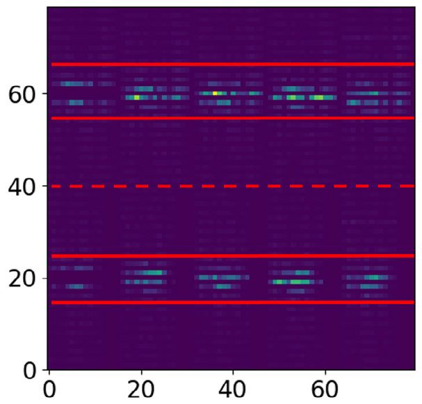
Y. Karayaneva et al.: Unsupervised Doppler Radar Based Activity Recognition for e-Healthcare

        FIGURE 9. The CAE architecture.

          FIGURE 10. The CVAE architecture.

are enforced to be close to a standard normal distribution,            The covariance matrix is given by:
which is measured by the regularisation term. Finally, both                                        n
                                                                                               1X
µφ and log σφ2 x are sampled to produce the compressed latent                           V=        (Xi − X)T (Xi − X)                            (8)
space representation z with the specified number of features.                                  n
                                                                                                  i=1
Considering the latent representation z, the decoder aims to           where n is the number of training samples and X = 1n ni=1 Xi
                                                                                                                                P
reconstruct x. The effectiveness of this operation is evaluated        is the average training image. It also has the size 80 × 80.
with the reconstruction loss.                                             More specifically, 2DPCA computes the covariance matrix
4) VARIATION-BASED PROJECTION TECHNIQUES                               only for the row or column dimension only. That is because
a: PRINCIPAL COMPONENTS ANALYSIS (PCA)                                 the initiall data is not vectorized to include all features. Con-
1D-PCA is known to be one of the most common linear                    sidering the 80×80 2D images in this study, only the columns
techniques for unsupervised feature extraction [60]. PCA               are used for computing the covariance matrix. This process is
finds the directions of main variations of data in the orig-           followed by eigen decomposition of the covariance matrix.
inal high dimensional space, and projects data along those             PCs retaining most of the variance are then selected. Similar
directions into a smaller sub-space. Based on this linear              to PCA, the first PC retains most of the variance.
projection, the dimensionality of data is reduced. In this
                                                                       D. CLUSTERING METHODS
paper, the Doppler radar data with 6400 variables are used
for PCA analysis. Based on a weighted linear combination               Two clustering methods are used for grouping the data sam-
of these features, the main directions of variations of data           ples. Both of the methods are distance-based: K-Means and
are calculated. In this paper, the s number of the first few           K-Medoids.
eigen vectors, explaining 95% of data variations, is used to
                                                                       1) K-MEANS
transform the original high dimensional data Dn×m Wm×s =
Zn×s . The first principal component (PC1) usually retains the         K-Means clustering is one of the most commonly used tech-
highest variance, which allows a smaller number of PCs to be           niques for unsupervised learning [62]. The K-Means method
selected.                                                              considers the number of groups or clusters K is known and it
                                                                       aims to group the data points based on their distances. In this
b: 2D PRINCIPAL COMPONENTS ANALYSIS (2DPCA)                            work, the Euclidean distance is used. The overall goal for the
PCA requires the 2D image matrix to be transformed to a 1D             clustering method is to group the data points D1 , D2 , . . . , Dn
image vector. This often leads to a high-dimensional image             in clusters by minimizing the intra-cluster distances. Intu-
vector. Therefore, the size of the covariance matrix V is              itively, the distances between data points from different clus-
extremely large. Logically, it becomes difficult to evaluate the       ters should be maximized. During training, K-Means outputs
covariance matrix considering the small number of training             the cluster centres ωk , where k = 1, 2, . . . , K , or also
examples. 2-dimensional PCA proposed in [61] allows the                known as centroids. The assignment of a new data point
covariance matrix to be calculated on the 2D images of size            to one of the clusters is such that, the sum of the squared
80 × 80. Hence, this corresponds to its smaller size, which            distances between the data point and all cluster centroids
has two main advantages. Less computation time is required             ω1 , ω2 , . . . , ωk are computed. Then, the sample is assigned
and the covariance matrix is more accurately evaluated.                to the cluster, where the corresponding distance is minimum.

62992                                                                                                                                VOLUME 9, 2021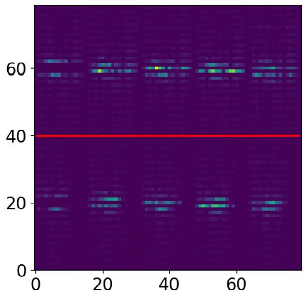
Y. Karayaneva et al.: Unsupervised Doppler Radar Based Activity Recognition for e-Healthcare

The objective function for K-Means, which specifies the                            similar positions, while the gap in the low dimensional space
sum of squared distances of each data point Di to cluster k,                       increases if the samples are non-similar. Hence, comparison
is defined as follows:                                                             measures will be extracted from this analysis, which can be
                         n X
                         X K                                                       useful for projects concerned about high-dimensional data
                   J=               rik ||Di − ωk ||2                    (9)       visualisation.
                          i=1 k=1
                                                                                   1) T-DISTRIBUTED STOCHASTIC NEIGHBOUR EMBEDDING
where rik is a binary function indicating the assignment of
                                                                                   (T-SNE)
data point Di to cluster k. If Di is assigned to cluster k,
                                                                                   T-SNE is a non-linear dimensionality reduction method,
the binary indicator rik = 1, and 0 otherwise:
                (                                                                  which has gained attention for its superior ability to visu-
                  1, if k = arg minj ||Di − ωj ||2                                 alise high-dimensional data by transforming it to a two or
          rik =                                        (10)                        three-dimensional space [64]. This method assigns each data
                  0, otherwise
                                                                                   point in a low-dimensional location by aiming to preserve
The overall aim is to minimize the J for values rik and ωk .                       the significance of the original information. Unlike linear
The procedure can be achieved by iterative optimization                            techniques such as PCA and SVD, t-SNE aims to keep similar
with respect to rik and ωk . In the first phase, the ωk is                         data points in close locations in the low-dimensional space.
fixed, while the goal is to optimize rik . The same notion is                      The superiority of t-SNE in comparison with other dimen-
applied to the second step as rik is fixed and the focus is                        sionality reduction methods is the ability to preserve the local
on the optimization of ωk . The entire process correspond-                         structure of the data as well as global information such as
ing to Expectation-Maximization algorithm is repeated until                        clusters. T-SNE has been recently compared with PCA for
convergence.                                                                       visualisation where the former achieved better visualisation
                                                                                   [65]. The steps for the t-SNE transformation are described
2) K-MEDOIDS                                                                       below:
K-Medoids is a clustering method based on distances anal-                             1) The Doppler sequences D1 , D2 , . . . , Dn are initially in
ysis, which has shown better performance for noisy and                                   their original 6400-dimensional space. T-SNE begins
problematic data than K-Means [63]. Similar to K-Means,                                  with determining the similarity between the data sam-
this method considers the number of groupings or clusters K                              ples. This is performed by computing their distances.
is known initially and K < n, where n is the number of data                              Euclidean distances are used in this study.
points. In contrast, K-Medoids considers a data sample for the                        2) The Euclidean distances are converted to probabilities
centroid or the medoid, which is not the case for K-Means. In                            describing normal distributions so that, similar data
the first step of K-Medoids, the algorithm aims to find a data                           samples have close values. On the other hand, dissim-
point Di in a cluster C(i) = k that is in minimum distance to                            ilar points have distinct similarity values. The simi-
the remaining observations in the cluster D0i . This distance is                         larity scores are calculated for each data points pair
denoted as ||Di −Di0 ||2 and the minimisation is shown in (11):                          Dij , where a similarity matrix is obtained based on
                                   n
                                   X                                                     probabilities pij .
                 i∗k = arg min            ||Di − Di0 ||2               (11)           3) The data samples are projected in a random order to the
                        i:C(i)=k C 0 =k
                                  i                                                      low dimensional space first. This results in a mismatch
Then, the output index i∗k is used to find a new centroid or                             with cluster patterns of data in the original domain
medoid, defined as ωk = Di∗k , k = 1, 2, . . . , K for all                               initially. The aim for t-SNE is to re-position the data
clusters.                                                                                samples in the new low dimensional space, such that the
   The second step of the method is to minimise the total error                          same clustering patterns of the high-dimensional space
by re-assigning each data sample to the closest centroid. The                            to be preserved.
clusters centroids are given ω1 , ω2 , . . . , ωK .                                   4) Then, the Euclidean distances between the data
                                                                                         samples are calculated in the lower dimensional
                   C(i) = arg min ||Di − ωk ||2                        (12)              space. Similarly, the distances are converted to a
                              1≤k≤K
                                                                                         t-Distribution (e.g. qij for the two data points Di and
Finally, step 1 and step 2 are iterated until the algorithm                              Dj ). t-Distribution is similar to normal distribution, but
converges to the optimum centroids.                                                      with taller tails. The taller tails of t-Distribution prevent
                                                                                         dissimilar data points to be positioned in close locations
E. VISUALISATION TECHNIQUES FOR                                                          of the lower dimensional space. The samples in lower
HIGH-DIMENSIONAL DATA                                                                    dimension are re-positioned using these probabilities
In this paragraph, three widely-known techniques for man-                                resembling distances. The re-positioning is performed
ifold learning are defined. The focus is on transforming                                 based on the two probabilities q of low dimension and
the very high-dimensional space in this dataset (Dn×m =                                  p of high dimension.
Dn×6400 ) to a 2-dimensional space. Manifold learning meth-                           5) t-SNE uses KL divergence to optimise the similarity
ods are known to map closely correlated data samples in                                  of the distributions described by q to those described

VOLUME 9, 2021                                                                                                                                  62993
Y. Karayaneva et al.: Unsupervised Doppler Radar Based Activity Recognition for e-Healthcare
by p. This can be interpreted as a constant comparison is reconstructed only by its neighbours, the weight function
of the samples distances in the lower-dimension to Wij = 0, if a sample XEj does not belong to the same class.
their distances in the original high-dimension. Then, Another constraint to the reconstruction loss is pthat the sum
re-positioning will be improved iteratively, as the sim- of the weight matrix’s rows should be one,
P
Wij = 1.
ilarity matrix of probabilities q is optimized using the j=1
original similarity matrix p. This sum-to-one constraint makes the weights invariant to
translation of the data points and their neighbors. The weights
2) MULTIDIMENSIONAL SCALING (MDS) are also invariant to rotation and scaling. The minimisation
MDS is a non-linear dimensionality reduction technique. of the loss function, allows computation of the weights W .
It can be used for visualization of high dimensional data They characterize the intrinsic geometric properties of each
in low dimensional space. It preserves the actual distances neighborhood.
of original samples in the low dimensional space. MDS Using the weights, Wij , it is possible to project each
considers dissimilarities of sample pairs contrary to other high-dimensional data point XEi to vector YEi of the lower
methods, which are concerned with similarities. Given the set representation based on another reconstruction cost function.
of observation D1 , D2 , . . . , Dn ∈ Rm , dij is the dissimilarities Having the Wij fix, the aim is to minimise the embedded
e.g. the Euclidean distance of two samples Di and Dj so that, cost function to optimise the low d-dimensional coordinates
dij = ||Di − Dj ||2 . MDS seeks z1 , z2 , . . . , zn ∈ Rk , so that (d < m):
k < m. A so called stress function is minimized for this aim n
X n
X
[66]–[68]: 8(Y ) = ||YEi − Wij YEj ||2 (15)
n
X i=1 j=1
Stress(z1 ,...,zn ) = (dij − ||zi − zj ||)2 (13)
i6=j III. EVALUATION AND RESULTS
In this section, the results obtained using the four
where ||zi − zj || is the Euclidean distance between zi and zj .
groups of unsupervised feature extraction techniques are
Then the pairwise distances are preserved in the lower
presented. These include the two proposed methods,
dimensional representation. A gradient descent algorithm is
namely, local DCT-based method and local entropy-based
used to minimize the stress function and find the compo-
method. In addition, the existing convolutional filter-based,
nents in the low dimension [68]. MDS transformation is
and variational-based projection methods are used for
monotone increasing with the increasing dissimilarities. The
comparison.
same notion is applied to growing similarities data, which
For local DCT-based method, local entropy-based method,
decreases the transformation. Hence, similar object pairs are
and 2DPCA, the inputs are n reshaped images of size 80×80.
positioned closely in the transformed space, while objects
In the case of CAE and CVAE, the inputs are n number of 3D
with dissimilarity are distinguished with larger distances.
cubes of size 2 × 100 × 32. While for PCA, the input data
3) LOCALLY LINEAR EMBEDDING (LLE)
is Dn × 6400. In the case of PCA and 2DPCA, the selected
number of eigen vectors preserves 95% of the data variance.
LLE is a non-linear dimensionality reduction method pro-
Leave-one-subject-out cross validation (LOOCV) is used
posed in [69]. The method is concerned with preserving the
to avoid over-fitting. As listed in Section II, four participants
global structure of the data based on an underlying manifold.
are included in the data. The four participants correspond to
The data are represented by n real-valued vectors XEi in a high
the four folds. The models are trained on three subjects data.
dimension m. i is the index of a sample. Each data point XEi , is a
Then, they are validated on unseen data from the remaining
member of a neighbourhood. Each neighbourhood consists
subject, which is not used for building the models. This is
of similar data points. Similar data points are expected to
repeated for all four subjects. Hence, Ztr = 150 × m is the
lie on a close locally linear patch of the smooth manifold.
training matrix and Zts = 50 × m is the matrix for testing,
The p nearest neighbours for each data point are defined by
where the number of features m varies for different models.
measuring the Euclidean distances. The local geometry of
In addition to the activities clustering results, the three
the patches can be characterised by linear coefficients. These
manifold learning methods t-SNE, MDS and LLE are com-
linear coefficients are used to reconstruct each data point from
pared in two scenarios. In the first scenario, they are used
its neighbours. The reconstruction loss is defined by:
to transform the raw data features to a 2-dimensional space.
n p
X X Since CVAE encoded features obtained the most accurate
(W ) = ||XEi − Wij XEj ||2 (14) clustering results, in the second visualization scenario, they
i=1 j=1
are used for projection into a 2-dimensional space.
where Wij are the weights defined for data points recon- True labels are only used for model evaluation and illustra-
struction using the corresponding neighbours. The number of tion purposes. The order of the predicted labels by clustering
samples is given as n, while the number of neighbours is p. is not necessarily consistent with the actual labels order.
The computed weights Wij correspond to the contribution of Therefore, the clustering accuracy is estimated by finding the
a data point XEj for reconstructing XEi . In order to ensure that XEi best-matching pairs of clusters labels and true labels. Based
62994 VOLUME 9, 2021Y. Karayaneva et al.: Unsupervised Doppler Radar Based Activity Recognition for e-Healthcare
FIGURE 11. (a) Illustration of the 40 × 40 local patches in the Doppler
spectogram. The optimum patch for feature extraction is ticked in green
color and (b) The corresponding Dunn’s index for the four 40 × 40 local
patches.
TABLE 1. Average and standard deviations of testing accuracies based on
K-Means and K-Medoids using DCT features from the raw data 80 × 80 FIGURE 12. Illustration of the Dunn’s index for the three patching
single patch and those from the selected 40 × 40 local patch features strategies used for feature extraction based on entropy analysis.
over 4 rounds of LOOCV.
on this, the predicted labels by clustering are matched to their
corresponding actual true labels. As such, a regular accuracy
score function is used for calculating the accuracy.
A. LOCAL DCT-BASED ANALYSIS RESULTS
FIGURE 13. (a) CAE and (b) CVAE robustness evaluation using Dunn’s
The proposed local DCT-based method extracts index.
non-overlapping square-sized patches from the original
80 × 80 2D map for analysis. Dunn’s index is used for
validating the method, which showed the highest values for The results of the Dunn’s indexes were computed using the
the 40 × 40 local patches. In Fig. 11a, the four possible K-Means clustering and presented in Fig. 12. As can be
non-overlapping patch locations for this size are illustrated. seen, the last patching strategy obtained the highest Dunn’s
Then, each 40 × 40 patch is divided into 3 × 3 sub-patches as index and therefore, it was selected for analysis. This result
was shown in Fig. 6 previously. Next, six DCT coefficients of was expected, because the last strategy considers a higher
the top-left zig-zag pattern are selected from each sub-patch number (10) of smaller patches. This represents local patterns
yielding a total of 9 × 6 = 54 DCT coefficients for each variations better compared to the other two strategies. The
40 × 40 patch. The features are then used for clustering. other two strategies consider a fewer number (2) of larger
The resulting Dunn’s indices are visualized and compared local areas, which leads to poorer entropy computation.
in Fig. 11b. As observed, the 40 × 40 patch in the top-left
corner of the 2D image is found as the best location in terms C. CAE AND CVAE ROBUSTNESS EVALUATION
of Dunn’s index for DCT analysis. That shows the lower order The two deep NN architectures CAE and CVAE are evalu-
frequencies coefficients are related to detection of activities. ated addressing two criteria: 1) the number of hidden layers;
In addition, DCT is applied on the original 80 × 80 image and 2) the number of extracted features as latent dimension.
so that, 54 DCT coefficients were selected similarly and used In regards to the number of hidden layers, two, three, and
for clustering. The results are compared with the proposed four hidden layers are considered. The latent dimension is
local patching strategy. Table 1 presents the average testing incorporated with the number of data samples in this study.
accuracies of the DCT analysis over the 4-subjects LOOCV The considered latent features are 50, 100, 150, and 200.
for the original image and the selected local patch. Since the study is unsupervised, the true labels are seen as
unknown. Hence, Dunn’s index is selected for measuring the
B. ENTROPY ANALYSIS RESULTS wellness of clusters separation. Fig. 13 reveals the Dunn’s
For the entropy analysis, the three patching strategies index for each experiment for CAE and CVAE.
depicted in Fig. 7 are considered. The first two strategies Based on the results presented in Fig. 13a, three hid-
resulted into 2-dimensional features, while the last patch- den layers with 50 extracted features are selected for CAE.
ing strategy resulted into 10-dimensional feature vectors. In regards to the CVAE architecture, two hidden layers
VOLUME 9, 2021 62995Y. Karayaneva et al.: Unsupervised Doppler Radar Based Activity Recognition for e-Healthcare
FIGURE 14. Confusion matrices for comparison between local FIGURE 15. Confusion matrices for CVAE encoded features using
DCT-Based+K-Means and local DCT-Based+K-Medoids for different K-Means (a) and K-Medoids (b) for different subjects.
subjects.
separability between the classes, while there are some
with 50 extracted features are selected based on the results overlapping clusters in the case of MDS and LLE.
presented in Fig. 13b. In order to perform comparison, the second scenario of
data visualisation is concerned by transforming the encoded
D. COMPARISON OF THE AVERAGE TRAINING AND data Dn×50 using t-SNE, MDS and LLE to a 2-dimensional
TESTING ACCURACIES FOR K-MEANS AND K-MEDOIDS space as seen in Fig. 17. Considering the illustration, all
USING ALL FEATURE EXTRACTION TECHNIQUES three methods showcase improvements in terms of cluster
The average training and testing accuracies with stan- separability. However, there is still overlapping between the
dard deviations over 4-subjects LOOCV for K-Means clusters. Since dimension reduction from 50 encoded features
and K-Medoids using all feature extraction methods are into only two features is a significant reduction in the number
illustrated in Table 2 and Table 3. of features, no accurate clustering is expected using these two
As it can be observed, the two superior architectures are the dimensional features. This is tested by applying K-Means and
local DCT-based frequency features extracted from the local K-Medoids on the two t-SNE features. The average testing
patches and CVAE encoded features. After that, the local accuracies are 42% and 45% for K-Means and K-Medoids
entropy analysis achieved the best results. K-Medoids has respectively. Hence, these manifold learning methods are
better performance than K-Means using the local DCT-based good for visualisation, but are not necessarily accurate for
coefficient features. On the other hand, CVAE encoded fea- clustering.
tures are better incorporated with K-Means. The results of
the K-Means and K-Medoids are very similar in the case IV. DISCUSSION
of local entropy-based features. In addition, CAE, PCA and The local patching strategy incorporated with DCT improved
2DPCA have worse performance, while 2DPCA shows a the average training and testing accuracies by 10%-15% for
minor improvement to PCA for K-Medoids. the two scenarios as seen in Table 1. It has been solely
In order to evaluate the two superior architectures’ per- validated using an unsupervised metric for the scope of
formance for different activity groups, confusion matrices this study. As such, the method can be applied for other
for K-Means and K-Medoids are visualised. The following supervised or unsupervised studies with Doppler radar data.
matrices in Fig. 14 consider the proposed local DCT-based The local patching strategies can even be improved when
method over 4-subjects LOOCV for K-Means (Fig. 14a) and used in a supervised framework, because the average vali-
K-Medoids (Fig. 14b). dation accuracies allow optimum estimation of the method’s
The confusion matrices for the CVAE encoded features parameters.
with K-Means clustering and K-Medoids clustering are visu- The confusion matrices for the architecture local
alised in Fig. 15a and Fig. 15b respectively. DCT-Based+K-Means and local DCT-Based+K-Medoids
Both feature extraction strategies results show confusion in Fig. 14 reveal that the activities walking (1) and jumping
of some activities. Further analysis of the results will be (3) are problematic as they are frequently confused. Similarly,
presented in the discussion section. the CVAE-based architecture in Fig. 15 shows confusion
between walking (1) and jumping (3). As it can be observed
E. VISUALISATION RESULTS from the confusion matrices, the walking (1), jumping (3)
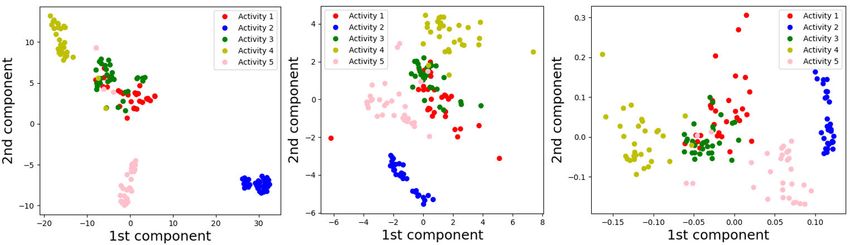
Visualization of the raw data and CVAE encoded features and standing (5) classes are seen as problematic. More data
are performed using t-SNE, MDS and LLE methods. Here, can be collected in order to improve the results with a higher
the actual data labels are used to map the samples. Ini- number of subjects. Considering the clustering methods,
tially, the original data Dn×m , where m = 6400, is trans- local DCT features are better incorporated with K-Medoids.
formed and visualised in a 2-dimensional space as shown On the other hand, the CVAE encoded features are more
in Fig. 16. As illustrated, t-SNE performs reasonable correctly clustered with K-Means. In addition, the results of
62996 VOLUME 9, 2021You can also read