CLASSIFICATION OF EXPANSIVE GRASSLAND SPECIES IN DIFFERENT GROWTH STAGES BASED ON HYPERSPECTRAL AND LIDAR DATA - MDPI
←
→
Page content transcription
If your browser does not render page correctly, please read the page content below
remote sensing
Article
Classification of Expansive Grassland Species in
Different Growth Stages Based on Hyperspectral and
LiDAR Data
Adriana Marcinkowska-Ochtyra 1, * , Anna Jarocińska 1 , Katarzyna Bzd˛ega 2
and Barbara Tokarska-Guzik 2
 1    Department of Geoinformatics, Cartography and Remote Sensing, Chair of Geomatics and Information
      Systems, Faculty of Geography and Regional Studies, University of Warsaw, 00-927 Warsaw, Poland;
      ajarocinska@uw.edu.pl
 2    Department of Botany and Nature Protection, Faculty of Biology and Environmental Protection,
      University of Silesia in Katowice, 40-032 Katowice, Poland; katarzyna.bzdega@us.edu.pl (K.B.);
      barbara.tokarska-guzik@us.edu.pl (B.T.-G.)
 *    Correspondence: adriana.marcinkowska@uw.edu.pl; Tel.: +48-2255-21507

 Received: 16 October 2018; Accepted: 10 December 2018; Published: 12 December 2018

 Abstract: Expansive species classification with remote sensing techniques offers great support for
 botanical field works aimed at detection of their distribution within areas of conservation value and
 assessment of the threat caused to natural habitats. Large number of spectral bands and high spatial
 resolution allows for identification of particular species. LiDAR (Light Detection and Ranging) data
 provide information about areas such as vegetation structure. Because the species differ in terms of
 features during the growing season, it is important to know when their spectral responses are unique
 in the background of the surrounding vegetation. The aim of the study was to identify two expansive
 grass species: Molinia caerulea and Calamagrostis epigejos in the Natura 2000 area in Poland depending
 on the period and dataset used. Field work was carried out during late spring, summer and early
 autumn, in parallel with remote sensing data acquisition. Airborne 1-m resolution HySpex images
 and LiDAR data were used. HySpex images were corrected geometrically and atmospherically before
 Minimum Noise Fraction (MNF) transformation and vegetation indices calculation. Based on a LiDAR
 point cloud generated Canopy Height Model, vegetation structure from discrete and full-waveform
 data and topographic indexes were generated. Classifications were performed using a Random
 Forest algorithm. The results show post-classification maps and their accuracies: Kappa value and
 F1 score being the harmonic mean of producer (PA) and user (UA) accuracy, calculated iteratively.
 Based on these accuracies and botanical knowledge, it was possible to assess the best identification
 date and dataset used for analysing both species. For M. caerulea the highest median Kappa was
 0.85 (F1 = 0.89) in August and for C. epigejos 0.65 (F1 = 0.73) in September. For both species, adding
 discrete or full-waveform LiDAR data improved the results. We conclude that hyperspectral (HS)
 and LiDAR airborne data could be useful to identify grassland species encroaching into Natura 2000
 habitats and for supporting their monitoring.

 Keywords: mapping; expansive grass species; hyperspectral; LiDAR; Natura 2000; Random Forest

1. Introduction
     Non-forest communities such as grasslands and meadows are recognized as the most species-rich
plant assemblages hosting numerous rare and endangered species. Increasing degradation of grassland
and meadow communities have been reported recently by many authors [1–3]. Among main reasons
responsible for the phenomenon of the abandonment of these habitats or intensification of management

Remote Sens. 2018, 10, 2019; doi:10.3390/rs10122019                    www.mdpi.com/journal/remotesensing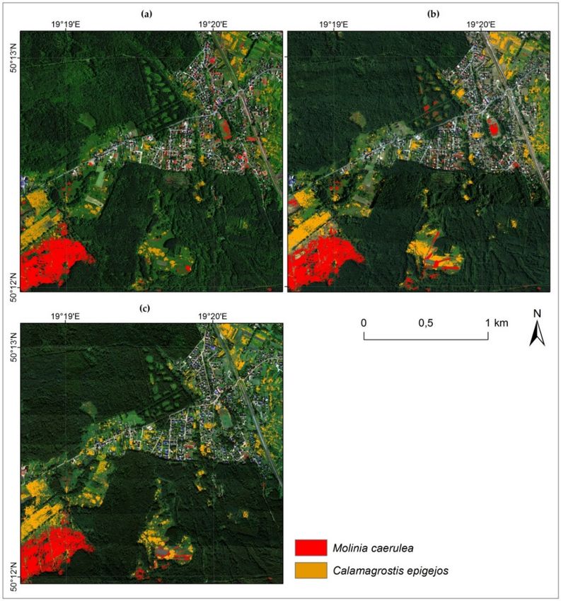
Remote Sens. 2018, 10, 2019                                                                          2 of 22

are mentioned. One of the manifestations of the disadvantageous changes in grassland and meadow
communities, including the ones important from a point of view of biodiversity conservation, is the
entering of expansive species which can dominate the community and considerably limit species
diversity. Calamagrostis epigejos and Molinia caerulea are listed among expansive species of global
importance due to their colonization of various ecosystems in Europe and North America, causing
grassland and meadow degradation [4–7].
      Research on the encroachment of alien invasive species into non-forest habitats is widely used
but also a large increase of native expansive species has been observed in many patches of non-forest
communities without proper management. Preserving the species-rich non-forest communities
requires monitoring of the state of their conservation values, in particular to detect any proliferation of
undesirable species.
      The fast and effective detection and mapping of invasive alien plants, and similarly
native expansive ones, at different spatial scales is becoming increasingly important for their
management [8–10]. Also monitoring the threat caused by invasive and expansive species in natural
habitats is essential for the process of the proper preservation of these habitats.
      The application of hyperspectral and ALS (Airborne Laser Scanning) remote sensing data is
a method complementary to traditional field surveys, which additionally allows coverage of large
areas [11]. It is probable that every plant species has a feature or a set of features which can be used for
its spectral identification. Achieving the expected result of marking out the appropriate time of spectral
data acquisition, in which the feature of the species is the most visible feature and simultaneously
enables it to distinguish itself from other species, is significant.
      Commonly, methods for mapping plant species are based on the subjective assessment of
the expert made in the field using the spot-map or line-transect methods. They are recognized
scientific methods, but during conducting mapping in the field they may be fraught with human
error. The disadvantages of these methods are that researcher is not able to explore the area of
research in a detailed way and the whole map of a bigger area has to be interpolated based on points
collected in the field, making the results imprecise. Remote sensing methods are more objective
because even if some errors in field data occur, the whole area is mapped in the same way. In some
cases, representatives of samples used for classification can be assessed by experts after obtaining first
classification results or using dominance profile graphs [12]. Nevertheless, remote sensing data ensure
measurability and verifiability, so they are reliable and, equally important, reproducible.
      Remote sensing offers many possibilities for vegetation research, from condition
analysis [13–17] to land use/land cover mapping including plant species or community
identification [18–20]. The electromagnetic spectrum covering the visible (VIS) and near infrared (NIR)
ranges is the most commonly used one for the analysis of vegetation [21]. Depending on the scale of
the study and the available resolution of remote sensing data, it is possible to identify plant units at
various levels: vegetation types, habitats, communities or species. Data from broad-band multispectral
scanners have successfully been used to classify land cover [22–24] or vegetation types [25,26].
For more complicated and complex units, such as habitats or plant communities, a higher spectral
resolution is needed to capture larger differences between them, and depending on the size of the unit,
satellite or aerial data may be used, which is related to the size of the pixel [19,27]. Hyperspectral data
consisting of hundreds of narrow spectral bands provides detailed information about analysed
objects [28]. It is a big advantage in comparison to more common multispectral data where in broad
several spectral bands the characteristics of these object are generalized. The importance is in the
possibility to differentiate analysed objects from the background. For particular species identification,
the most suitable method involves airborne imaging spectroscopy data consisting of hundreds of
spectral bands which allows for the detection of spectral signatures of particular plants relative to their
background of surrounding vegetation and their high spatial resolution provides the detail needed for
patch identification [18]. Because of these valuable hundreds of bands, hyperspectral data processing
is more challenging and storage demanding. To make hyperspectral data processing more operational,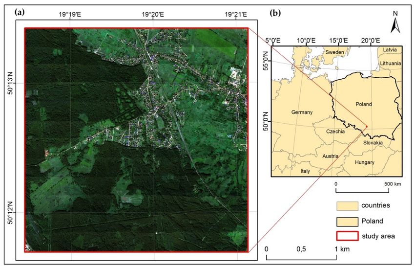
Remote Sens. 2018, 10, 2019                                                                         3 of 22

different transformation approaches are used, the most commonly used are Principal Component
Analyses (PCA) [29] or Minimum Noise Fraction (MNF) [30].
     Different classifiers are used for plant identification, the choice of which is related to the remote
sensing data type mentioned above, as well as the scope of the study. Traditional classifiers are used
to classify more general units, such as land cover, which includes vegetation cover mapping [31].
Often, remote sensing vegetation indicators, such as normalized difference vegetation index (NDVI),
are included in the classification, especially in multi-temporal analyses, insofar as they are good
indicators for reflecting periodically dynamic changes of vegetation groups [32,33]. Machine learning
methods, such as Random Forest and Support Vector Machines (SVM), are successfully used to
identify both communities and species [19,20,34,35]. Comparative analysis of methods used to classify
particular species presented higher accuracies reached for a Random Forest algorithm [36–38], which is
better than SVM because of processing time.
     In the literature, there are many examples of applications of hyperspectral remote sensing for
species detection, a significant part being devoted to the identification of tree species [38–40]. A large
group consists of classifications of invasive plants that pose a threat to native vegetation [18,41–43].
There are few studies using remote sensing techniques to identify expansive species that, although
native, are also threatening to natural habitats. Scientists analysed C. epigejos and M. caerule spreading
using statistical methods [44,45]. Several authors used hyperspectral images to identify particular
species encroaching into heathlands: M. caerulea entering the Natura 2000 habitat classification was
addressed by Mücher et al. [46] in the areas of Ederheide and Ginkelse heide in the Netherlands and
by Haest et al. [47] in Kalmthouse Heide in Belgium. C. epigejos was mentioned by Schmidt et al. [48]
in Oranienbaum Heath located near Dessau in the Elbe-Mulde-lowland in Saxony-Anhalt in Germany,
but only with encroaching into heathlands being the main object of the study. The specific features
of this species have not been studied more deeply. Separating different spectrally similar classes
as grassland types using narrowband images is supported by Ali et al. [49], who underlines the
possibility to obtain them from the airborne level, due to the lack of spaceborne hyperspectral sensors
currently in orbit and also higher spatial resolution. Based on Mücher et al. [46] collecting more
images over the growing season and incorporation of vegetation information from LiDAR data
might be helpful in grasses differentiation. Multi-temporal analyses using satellite data were used by
researchers to identify invasive species [50,51] or grasslands [33,52]. Separability of grassland classes
were supported by characteristic phenological development of individual habitat classes as greenness
or colouring in the blooming phase using optical RapidEye data and vegetation height and structure
from radar backscatter using TerraSAR-X data [33]. Seasonal effect on tree species classification was
also analysed based on hyperspectral Airborne Imaging Spectrometer for Applications and LiDAR
data [53]. LiDAR data are known as being useful for mapping canopy structure, but rarely as an
alternative to the imaging vegetation classification method [54]. It is more commonly is used with other
types of data from spaceborne [55] or airborne [56] levels. While LiDAR with hyperspectral data were
most commonly used in classification of trees [39,57,58] or shrubs [59], several studies of non-forest
vegetation [60] including also only LiDAR [54,61] were also presented. Separating higher vegetation as
trees or shrubs from lower vegetation [62] is much easier than capturing smaller differences in lower
species from higher vegetation, but in grassland mapping of the lowland hay meadows Natura 2000
area [54], the strong potential of vegetation high-dependent variables was noticed. Using only LiDAR
derivatives as terrain height models for predictive modelling of non-forest communities locations was
presented by Ward et al. [63]. However, other authors by adding passive optical data to LiDAR data
obtained higher classification accuracy [64,65] in vegetation analysis due to possibility to differentiate
features such as lignin composition, senescent matter or soil presence [66]. The combination of high
and spectral data could provide complementary information about the study object and optimize their
strengths [65,67]. The vast majority of classifications present single training and validation data split
but they can induce biased results [68]. Iterative accuracy assessment was proposed by several authors
in the classification of trees [39,40,69] and non-forest vegetation [20,27]. This approach allows for more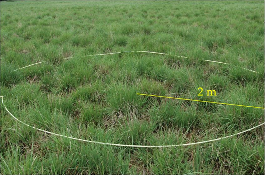
Remote Sens. 2018, 10, 2019 4 of 22
objective conclusions, avoiding very poor or very good results obtained by chance. It is important
especially when comparing different scenarios, datasets, or classifiers.
Objectives
Although in a number of studies, characteristic features of the targeted species such as phenology,
colours of flowers, physiological traits and form of growth have been used for their detection, optimal
methodologies still remain to be defined. Because the literature lacks the use of hyperspectral
with LiDAR data for grassland species identification, this aim remains necessary. Referring to this,
the objective of this study is to investigate the use of HySpex data and LiDAR products to classify
the two expansive grass species C. epigejos and M. caerulea in Natura 2000 habitats, which have been
recognized as aggressive competitors with the tendency of dominating the plant community, causing
negative changes in its structure and species composition. More specifically, the investigation aims to:
• compare different times of airborne data acquisition depending on the growing phase of analysed
species, to point out the most optimal time of proper species detection,
• collate different datasets containing spectral data and additional different vegetation with high
layers to choose the most optimal dataset to detect these species.
The presented approach intends to compare these elements with respect to the maximum
classification accuracy reached and botanical assessment leading to selecting the most optimal data
needed to provide good material for the monitoring of Natura 2000 areas.
2. Data and Methods
2.1. Study Area and Object of the Study
The study area is located in the Silesia Upland in southern Poland under the administrative boundary
of Jaworzno town (Figure 1). This part of the town is called Ci˛eżkowice-Pod Łużnikiem (central part
of the map) and Ci˛eżkowice (in the northeast part). The vegetation of the study area is a mosaic of
planted forest and various types of non-forest plant communities such as grasslands and wet meadows.
Our investigations were carried out in non-forest plant communities, mainly wet meadows, still species-rich
(southern part of the map) and grassland at the hills in Ci˛eżkowice (eastern part).
In this part of town, a special area of conservation of Nature 2000 habitats “Meadows in
Jaworzno” PLH240042 was appointed for the conservation of natural habitats: wet meadows (Molinion)
(code: 6410), lowland hay meadows (Arrhenatherion elatioris) (code: 6510) and of species of butterflies:
Maculinea (Phengaris) nausithous (code: 6179), and Maculinea (Phengaris) teleius (code: 6177).
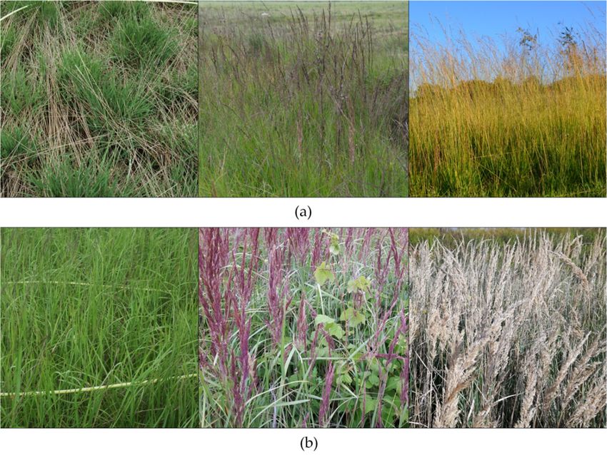
As the object of the study two grass species were selected, namely M. caerulea and C. epigejos (Figure 2).
Both species belong to native elements in the flora of Poland. They are classified as expansive species and
differ in terms of many features, including the type of growth. Expansive species are defined as native
species that increase their distribution and colonize new habitats in a geographical area where they are
native (they have localities of native occurrence within the same area [70]). According to the definitions
accepted for the purpose of this study, native expansive species quickly spread and colonise new areas,
in general common plant species, posing a threat as a result of the secondary inheritance for rare plant
communities, by often appearing to reduce the biodiversity of natural habitats [71].
M. caerulea (Purple Moor-grass) is a species from the family Poaceae, native to Europe, west Asia,
and north Africa. It is an erect, compactly tufted perennial grass, 50–90 cm high, forming either tussocks or
extensive swards. Rootstock is more or less creeping, with both stout and fine roots. Leaf blades are flat,
3–8 (max. 10) mm wide, with a bluish-green colour. Panicles are erect, ranking from very dense to open
and very loose, dark to light purple, brownish, yellowish, or green with more or less raised branches, 15 cm
long. The long narrow purple spikelets are a major identification feature. Fruits have a length of 2 mm.
Flowering and fruiting occur in late June or early July to mid-September. Its range of habitats includes wet
meadows, heaths, montane grassland, bogs and open woodland. The common features of these habitats,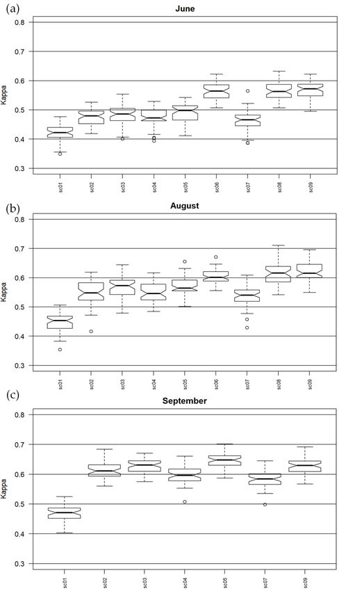
Remote Sens. 2018, 10, 2019 5 of 22
particularly in the area where M. caerulea is found, is permanently or seasonally wet ground. M. caerulea is
Remote
Remote Sens.
Sens. 2018,
2018, 10,10, x FOR
x FOR PEER
PEER REVIEW
REVIEW 5 5of of
2222
a very variable species among others owing to variation in overall size, in the length and width of leaves,
and especially
size,ininthe in the length,
thelength
length width
andwidth
width and colour of the panicles. M. caerulea is cultivated for its panicles of
size, and ofofleaves,
leaves, andespecially
and especially
ininthe
thelength,
length, widthand
width and colourofofthe
colour thepanicles.
panicles.
purpleM.spikelets
caerulea on
is yellow
cultivated stems
for its [72,73].
panicles of purple spikelets on yellow stems
M. caerulea is cultivated for its panicles of purple spikelets on yellow stems [72,73]. [72,73].
Figure
Figure
Figure 1. 1. Location
1. Location
Location of
ofofthe the
the study
study
study area
area
area atatthe
at the
the local
local
local scale
scale
scale (a):
(a):
(a): basemap:
basemap:
basemap: HySpex
HySpex
HySpex image
image inin
image natural colour
in natural
natural colour colour
Red, Red,
Red, Green,
Green,
Green, Blue Blue (RGB)
(RGB)
Blue composition,
(RGB)composition, acquired in September
acquiredininSeptember
composition, acquired September 2016
2016
2016 with relating
withwith to
relating
relating a map
to a of
to a map of
map Central
of Central
Central
Europe
Europe
Europe (b):
(b):(b):
© © EuroGeographics
EuroGeographics
© EuroGeographics forfor
for the
the
the administrative
administrative
administrative boundaries.
boundaries.
boundaries.
Figure
Figure 2. 2. 2.Molinia
Figure Moliniacaerulea
Molinia caerulea(a):
caerulea (a):
(a): left—vegetative phase,
left—vegetative
left—vegetative phase, middle—blooming,
phase, right—fruiting,
middle—blooming,
middle—blooming, and
right—fruiting,
right—fruiting, and
Calamagrostis epigejos (b): left—vegetative phase, middle—blooming, right—fruiting.
and Calamagrostis epigejos (b): left—vegetative phase, middle—blooming, right—fruiting.
Calamagrostis epigejos (b): left—vegetative phase, middle—blooming, right—fruiting.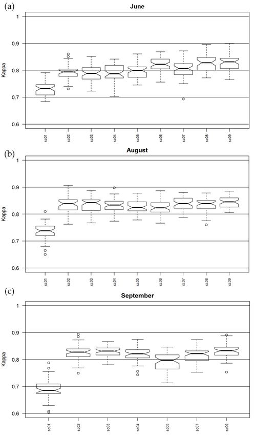
Remote Sens. 2018, 10, 2019                                                                                6 of 22

     C. epigejos (Wood Small-red) is a tall caespitose perennial grass from Poaceae family, widely
distributed in, and native to, Eurasia and expanded its range also in North America. The plant forming
tufts or tussocks, 60–200 cm, high, with creeping rhizomes. The culms are erect or slightly spreading,
usually unbranched. Leaf blades flat, stiff, and hairless, 4–14 (max. 20) mm wide, with dull grey-green
colour. Panicles erect, lanceolate to oblong, very dense before and after flowering, 15–30 cm long,
3–6 cm wide, purplish, brownish, or green. Spikelets are densely clustered, narrowly lancelolate
or finally gaping. Their fruits have a length of 1 mm. Flowering and fruiting occurs in late June to
mid- or late September. Culm height, leaf length, width, shape, and colour are very variable and
depend on site factors, especially the light climate or water capacity. Natural habitats supporting C.
epigejos include sand dunes, river floodplains, fens, steppes and subalpine grassland but the species is
particularly abundant in dry, open grassland that is usually ungrazed, forests, clear cut forest, along
railway lines, roadsides and on urban and industrial wasteland. C. epigejos grows on dry, and on
flooded soils, but prefers more dry areas than M. caerulea [4,72–74]. It is a competitively strong species,
which is able to dominate the colonized sites. The plants have two types of clonal growth. The first,
intra-vaginal ramet formation, creates groups of closely attached and connected ramets, which we
further call “clumps”. The other way is formation of extravaginal ramets on rhizomes of several
decimeters length [75]. Strong underground rhizomes of C. epigejos can spread up to several meters
in one direction, forming dense stands/patches and often caused negative changes in structure and
species composition of native plant communities [76,77].

2.2. Remote Sensing Data
     Remote sensing data come from instruments that are components of an aerial remote sensing
platform, built as part of the HabitARS project by MGGP Aero Company. One of them is the HySpex
scanner (Norsk Elektro Optikk, Oslo, Norway), acquiring data with a spatial resolution of 1 m,
registered in 470 spectral bands in two ranges of electromagnetic spectrum: Visible and Near Infrared
(VNIR, 400–1000 nm) and Shortwave Infrared (SWIR, 930–2500 nm) with 3.26 and 5.45 nm spectral
sampling, respectively (Table 1). The sensor has 16-bit radiometric quantization.

                                 Table 1. Main technical parameters of HySpex scanner.

                                                                                 Scanner
                                        Characteristics
                                                                           VNIR          SWIR
                                        Spatial pixels                      1800           384
                                 Minimum wavelength [nm]                     416           954
                                 Maximum wavelength [nm]                    995            2510
                                   Spectral sampling [nm]                   3.26           5.45
                                        No. of bands                    182 (163 1 )       288
                                 Radiometric resolution [bit]                16             16
                                   Field of view (FOV) [◦ ]                17–34          16–32
                            Instantaneous field of view (IFOV) [◦ ]      0.01–0.04      0.04–0.08
                    1   Selected number of bands because of overlapping spectral ranges between sensors.

     The second element of the platform is IGI Lite Mapper 6800 system (Integrated Geospatial
Innovations, Kreuztal, Germany), which consists of the Riegl LMS-Q680i Airborne Laser
Scanner, from which data was gathered with a point-cloud density of 7 points/m2 (Table 2).
Additional component was DigiCAM39 RGB camera (Integrated Geospatial Innovations, Kreuztal,
Germany) with 10 cm spatial resolution. Within HabitARS project, the data were acquired in 2016 and
2017. In 2016 it was 21 June, 23 July and 10 September and for 2017 9 June and 11 August. Analyses of
data quality allowed for selection of the data from September 2016 and June and August 2017.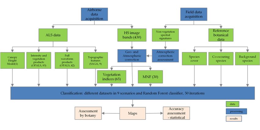
Remote Sens. 2018, 10, 2019                                                                                                   7 of 22

   Remote Sens. 2018, 10, x FOR PEER  2. Main technical parameters of Lite Mapper 6800.
                                TableREVIEW                                                                               7 of 22

                                       Characteristics
                                      Wavelength     [nm]                      Riegl LMS-Q680i
                                                                                     1550
                                     Pulse   duration
                                      Wavelength    [nm][ns]
Remote Sens. 2018, 10, 2019 8 of 22
greenness, narrowband greenness, canopy nitrogen, canopy water content, dry or senescent carbon,
leaf pigments and light use efficiency.
Processing of LiDAR data consisted of georeferencing, extraction, filtering and classification
of point cloud. The point cloud orientation was proceeded using the RiProcess package [82]
(Horn, Austria) in Riegl software and the accuracy was assessed at 0.01 cm level of 1 sigma. In 2016,
the data were processed into discrete (DISC) type and in 2017 to discrete and additionally to
full-waveform (FWF), which provided more information about the targets in the footprint than
only location [83]. Full-waveform information was used during postprocessing of raw FWF files to
gain more data about vegetation. In order to do this the threshold value was empirically defined
(as 3) and used in RiAnalyze software [84] (Horn, Austria). Apart from the threshold, amplitude and
pulse width extra byte was used as an additional structural metric for classification, derived using
the Riegl RiProcess. The point cloud was classified to ground, noise and vegetation classes using
TerraSolid software [85]. Processed point cloud was used to create Canopy Height Model (CHM)
and vegetation structure data (Table S1 in Supplementary Materials) in OPALS (Orientation and
Processing of Airborne Laser Scanning) software [86] (Vienna, Austria). On the basis of the point cloud,
the Digital Terrain Model (DTM) was calculated interpolating points in ground class using moving
planes in two iterations. During this process, the following rasters were also calculated: sigmaZ,
slope, exposition and Digital Surface Model (DSM), which was calculated by interpolating points from
class ground and vegetation (using points with highest z values for each raster cell). The CHM was
calculated using a differential model from DSM and DTM created from the ground and vegetation
classes. Rasters were calculated on all points with 1 m resolution, classified as ground and classified
as vegetation. Finally we calculated 83 discrete rasters that contained different statistics (maximum,
minimum, median, mean, range, root mean square, variance) of amplitude, echo ratio and normalized
height (Z), exposures, slopes and sigma on Digital Terrain Model and Digital Surface Model, as well
as point density and vegetation cover which means the number of returns classified as vegetation
divided by the number of all returns multiplied by 100. Full-waveform rasters in the number of
42 contained previously mentioned statistics calculated amplitude and pulse width, and also for
all points, ground and vegetation. Topographic indexes (TOPO) were also generated using Terrain
analysis package of SAGA software [87] (Hamburg, Germany) and they were: Topographic Position
Index, Topographic Wetness Index, Direct Insolation, Slope, Aspect, Module Multiresolution Index of
Valley Bottom Flatness, Multi-resolution Ridge Top Flatness and Modified Catchment Area.
Selected MNF bands were combined with calculated indices and LiDAR derivatives in ENVI
using Layer Stacking. The datasets were called scenarios, with corresponding number listed in Table 3.
The dataset consisting original mosaic of spectral bands called sc01 was also created to check if the
original or transformed data will perform better, which is important from an operational point of view.
Table 3. Used datasets (MOSAIC—mosaic of spectral bands, MNF—MNF transforms, CHM—Canopy
Height Model, VIS—vegetation indices, DISC—discrete LiDAR data, FWF—full-waveform data,
TOPO—topographic indices).
Scenario No. Dataset
sc01 MOSAIC
sc02 MNF
sc03 MNF+CHM
sc04 MNF+VIS
sc05 MNF+DISC
sc06 MNF+DISC+FWF 1
sc07 MNF+TOPO
sc08 MNF+FWF1
sc09 MNF+CHM+VIS+DISC+FWF1 +TOPO
1 Excluded from September.Remote Sens. 2018, 10, x FOR PEER REVIEW 9 of 22
Remote Sens. 2018,Botanical
2.3. Reference 10, 2019 Data 9 of 22
Simultaneously with the acquisition of airborne data, on-ground botanical reference data were
2.3. Reference
obtained threeBotanical Data the growing season (spring, summer and autumn) with the purpose of
times during
assessing the species with
Simultaneously detection possibilities
the acquisition of at different
airborne phases
data, of the life
on-ground cycle, on
botanical researchdata
reference areas (of
were
average size 5 km 2), where these species occurred at diverse frequencies and cover. The data collected
obtained three times during the growing season (spring, summer and autumn) with the purpose
were
of used tothe
assessing identify
species species characteristics
detection possibilities such as percentage
at different phases cover in life
of the reference
cycle, polygons,
on research growth
areas
stage,
(of flowering
average size 5and kmfruiting
2 ), where stage,
thesediscoloration/damage,
species occurred at diverse list of co-occurring
frequencies and species in particular
cover. The data
that havewere
collected coverused
above 20%, andspecies
to identify additional information,
characteristics suchi.e.,
as% of bare ground,
percentage cover in%reference
of vegetation, % of
polygons,
mosses and
growth % of
stage, litter (necromass)
flowering and fruiting andstage,
type of land use (mowing, pasturage).
discoloration/damage, For eachspecies
list of co-occurring of the in
plant species analysed, at least 100 reference 2-m buffer polygons (Table
particular that have cover above 20%, and additional information, i.e., % of bare ground, % of 4, Figure 4) were gathered
together with
vegetation, % ofa mosses
similarand number of reference
% of litter (necromass) polygons for of
and type surrounding vegetation
land use (mowing, or otherFor
pasturage). species
each
with similar morphology or with frequently coexisting species (e.g.,
of the plant species analysed, at least 100 reference 2-m buffer polygons (Table 4, Figure 4) were Solidago canadensis and S.
gigantea). These polygons were treated as a “background” class, which
gathered together with a similar number of reference polygons for surrounding vegetation or other were reference 2-m buffer
polygons, established in the patch of the species not chosen regarding the invasion/expansion in
species with similar morphology or with frequently coexisting species (e.g., Solidago canadensis and
the plant community, provided that an examined species is not acting in it or covering it doesn’t
S. gigantea). These polygons were treated as a “background” class, which were reference 2-m buffer
exceed the 10%. All data were stored in GNSS receiver Spectra Precision GPS MobileMapper 120
polygons, established in the patch of the species not chosen regarding the invasion/expansion in
(Spectra Geospatial, Westminster, CA, USA) and in traditional field data form and finally in the
the plant community, provided that an examined species is not acting in it or covering it doesn’t
database. Additionally, to the database were joined polygons of “background” class drawn
exceed the 10%. All data were stored in GNSS receiver Spectra Precision GPS MobileMapper 120
manually based on orthophotomaps from RGB camera, referred to as “forest” and “shadow” (in
(Spectra Geospatial, Westminster, CA, USA) and in traditional field data form and finally in the
the number of 30 per class).
database. Additionally, to the database were joined polygons of “background” class drawn manually
based on orthophotomaps from RGB camera, referred to as “forest” and “shadow” (in the number of
Table 4. Number of collected polygons.
30 per class).
Species Polygons June 2017 August 2017 September 2016 1
species from field Table 4. Number of collected234
measurements polygons. 256 245
Species background from
C. epigejos
field measurements June662
Polygons 2017 August6792017 September6142016 1
species selected 2
species from field measurements
222
234 256
241 245
237
background
background selected
from field 2
measurements 643
662 679660 614614
C. epigejos 2
species from species
fieldselected
measurements 222
195 241198 237197
background selected 2 643 660 614
background from field measurements 656 737 654
M. caerulea species from field measurements 195 198 197
species selected 2
background from field measurements
174
656 737
183 654
177
M. caerulea background selected 649 728
species selected 2 2
174 183 177649
background selected2 649 728 the changes 649
1 The dates are not ordered chronologically, but phenologically to present in growing
1 The dates are not ordered 2 Polygons
season. Polygons
2 afterchronologically,
assessing thebut phenologically
correctness, to present
similarity the changes
analysis andinfor
growing season.
analysed species also
after assessing the correctness, similarity analysis and for analysed species also with more than 40% of species cover.
with more than 40% of species cover.
Figure 4.
Figure 4. The 2-m buffer polygon
polygon of
of M.
M. caerulea.
caerulea.
The first
first step
step of
of validation
validation of
of reference
reference data
data was
was assessing
assessing the
the correctness
correctness of
of polygons
polygons which
which
means
means the
theremoving
removingofof shadowed
shadowed or mowed polygons
or mowed of species.
polygons TheseThese
of species. types types
of errors
of could
errorsbe caused
could be
by collecting ground botanical data few days after aerial data acquisition. The next step of
caused by collecting ground botanical data few days after aerial data acquisition. The next step ofpreparing
the reference data was an analysis of mistakes and errors. The aim of this stage was to capture errorsRemote Sens. 2018, 10, 2019 10 of 22
from the database related to the incorrect entry of the name of the site by the botanical team during
field measurements or the recognition of the site, where there are species strongly related to other
classes—also mistakes from the field. This kind of error could not be discovered in the early steps.
Based on a t-distributed stochastic neighbour embedding (t-SNE) machine learning algorithm, the most
spectrally homogeneous groups of polygons without errors were selected [88]. It is a non-linear data
size reduction technique that simplifies multi-dimensional space down to two or three dimensions.
The analysis was performed on the basis of 30 MNF bands in R software [89]. In this way, the similarity
of reference sites between classes was determined on the basis of remote sensing data. On the basis of
analysis of the botanical database, outliers were determined by botanists, which should be removed
from further analyses. As a result, 14 errors were found in polygons gathered in September 2016 for
C. epigejos. Finally, for evaluating the performance of the classification method, the ratio of the total
area of used reference data collected to the study site area (excluding mask of urban land cover) was
calculated and it was the following: 0.001973 for both M. caerulea and C. epigejos classification in June;
0.002186 for M. caerulea and 0.002175 for C. epigejos in August and 0.001994 for M. caerulea and 0.001948
for C. epigejos in September.
2.4. Random Forest Classification and Accuracy Assessment
To acquire information about the best dataset and time of data the Random Forest decision tree
ensemble classifier [90] was used. In each classification two parameters were used: ntree (number of
trees) equal to 100 and mtry (number of features randomly sampled as candidates at each split) equal
sqrt (n_features), where n_features was the number of used layers in the classification. The mtry value
was set as a default value and also to make it possible to analyse all features in each tree [37]. This was
done separately for C. epigejos and M. caerulea—in each classification two classes were classified (species
and background). To make the information more objective, the classification was performed 50 times
for each dataset and campaign. The field data were randomly sampled using 50/50% of training and
validation split. Based on the previous experiments only species with greater than 40% covered in
polygons were chosen as study objects.
The results for single classification and set of classifications were compared based on the
Kappa statistic [91,92] which is the common method of evaluation in machine learning classification
problems [37,93]. The nonparametric U Mann-Whitney-Wilcoxon test was used to evaluate the
statistical significance of the differences in Kappa accuracy between classifications with different
scenarios. Significant differences between the groups were assessed at p = 0.05. The user (UA) and
producer (PA) accuracies for species and background were calculated and then the weighted mean of
both values as F1 statistics were combined [94]. For the best Kappa values in each classification set,
the maps of species distribution were produced, and the confusion matrix was analysed.
3. Results
The results were presented on the maps (Figure 5) and calculated accuracies (Figures 6 and 7).
The Kappa accuracy obtained for the classification in each campaign was presented in boxplots.
Datasets for differences that were not statistically significant were listed in Table S2 in Supplementary
Materials. Because sc01 contains a mosaic of all spectral bands, the differences between it and the other
scenarios in which MNF channels were used are significant. For Molinia in June, the highest Kappa
accuracy (around 0.83) was obtained for a group of sets that used MNF transforms and full-waveform
products from LiDAR, as well as for MNF with all additional layers (sc09), a slightly lower accuracy
for pairs: MNF + topographic indexes and MNF + discrete data from LiDAR (approx. 0.81). For the
group in which the MNF alone and MNF bands with VIS and CHM were used, the Kappa median
value was lower (0.79) and these scenarios presented the most diversified values obtained during
50 iterations. In August, the accuracy for Molinia was more stable and reached the highest level.
Aside from sc01, all medians were higher than 0.8. The best set included MNF with topographic
indices and full-waveform data; in contrast, the lowest level of dispersion of results was obtainedRemote Sens. 2018, 10, 2019 11 of 22
Remote Sens. 2018, 10, x FOR PEER REVIEW 11 of 22
for all additional layers from MNF (sc09). The scenario containing the MNF bands alone was not
statistically
statisticallydifferent
differentfrom other
from MNF
other scenarios,
MNF but it but
scenarios, had the highest
it had the level of dispersion.
highest In September,
level of dispersion. In
the differences
September, thebetween databetween
differences sets for Molinia were
data sets formuch higher
Molinia werethan in August.
much higher The
thanhighest accuracy
in August. The
was obtained
highest for was
accuracy MNF, MNF +for
obtained CHM andMNF
MNF, MNF+ with
CHMall andadditional
MNF with layers, but the lowest
all additional layers,level of
but the
dispersion was observed for sc03. A pair of data sets with discrete data of the lowest values
lowest level of dispersion was observed for sc03. A pair of data sets with discrete data of the lowest and the
highest levelthe
values and of highest
value dispersion standdispersion
level of value out in particular.
stand out Forinsc01, the Kappa
particular. median
For sc01, the was themedian
Kappa lowest
(0.69).
was the lowest (0.69).
Figure 5.
Figure 5. The results obtained
obtained for
for June
June (a),
(a), August
August (b)
(b) and
and September
September (c).
(c).
Accuracy speciesand
Accuracy for species andbackground
backgroundwas wasalso
also calculated
calculated forfor
thethe result
result obtained
obtained during
during the
the best
best iteration. It was a combination of producer and user accuracy, which is referred
iteration. It was a combination of producer and user accuracy, which is referred to as the F1 value. to as the F1
value.
For M.For M. caerulea
caerulea (Table
(Table 5), this
5), this accuracy
accuracy confirms
confirms thethe accuracy
accuracy ofofKappa—the
Kappa—thelowest lowest values
values were
were
obtained
obtained for
for June.
June. The best dataset in June was sc08, where F1 reached reached 0.87;
0.87; the
the lowest
lowest value
value was
was for
for
sc01 (0.72). In general,
sc01 (0.72). general, F1 accuracies were the best in August, most of the median values
accuracies were the best in August, most of the median values for scenariosfor scenarios
was
was0.86,
0.86,the
thehighest
highestwas
was0.89 forfor
0.89 sc09 and
sc09 even
and evensc01 consisted
sc01 of mosaic
consisted of spectral
of mosaic data data
of spectral was also
washigh
also
and reached a 0.84 value. September was the second highest in term of class accuracies
high and reached a 0.84 value. September was the second highest in term of class accuracies and here and here the
best was also sc09 with 0.88 value, next was sc04 and 05 with 0.87 value. A slightly
the best was also sc09 with 0.88 value, next was sc04 and 05 with 0,87 value. A slightly lower value lower value for
sc08 (0.82)
for sc08 waswas
(0.82) noticeable.
noticeable.Remote Sens. 2018, 10, 2019 12 of 22
Remote Sens. 2018, 10, x FOR PEER REVIEW 12 of 22
Figure 6. M. caerulea
Figure Kappa
6. M. caerulea accuracies
Kappa calculated
accuracies forJune
calculated for June(a),
(a), August
August (b) and
(b) and September
September (c). (c).
Table 5.Table
User,5. producer
User, producer and F1 values of M, caerulea and background for the best iteration of Kappa.
and F1 values of M. caerulea and background for the best iteration of Kappa.
June August September
sc. No. Class
JuneUA PA F1 UA PAAugust F1 UA PA F1 September
sc. No. Class M. caerulea 0.88 0.61 0.72 0.89 0.79 0.84 0.85 0.67 0.75
sc01 UA PA0.93 F1 0.96 UA 0.98 PA
background 0.98 0.95 0.97 0.94 F1
0.98 0.96UA PA F1
Molinia caerulea 0.88 0.79 0.83 0.88 0.77 0.82 0.91 0.81 0.86
M. caeruleasc02 0.88 0.61 0.72 0.89 0.79 0.84 0.85 0.67 0.75
sc01 background 0.96 0.98 0.97 0.95 0.98 0.96 0.97 0.99 0.98
background 0.93 0.98 0.96 0.95 0.98 0.97 0.94 0.98 0.96
Molinia caerulea 0.88 0.79 0.83 0.88 0.77 0.82 0.91 0.81 0.86
sc02
background 0.96 0.98 0.97 0.95 0.98 0.96 0.97 0.99 0.98
M. caerulea 0.92 0.75 0.82 0.89 0.83 0.86 0.87 0.8 0.84
sc03
background 0.95 0.99 0.97 0.96 0.98 0.97 0.96 0.98 0.97Remote Sens. 2018, 10, 2019 13 of 22
Table 5. Cont.
June August September
sc. No. Class
UA PA F1 UA PA F1 UA PA F1
M. caerulea 0.92 0.72 0.81 0.9 0.83 0.86 0.93 0.81 0.87
sc04
background 0.95 0.99 0.97 0.96 0.98 0.97 0.97 0.99 0.98
M. caerulea 0.92 0.73 0.81 0.94 0.79 0.86 0.93 0.82 0.87
sc05
background 0.95 0.99 0.97 0.96 0.99 0.97 0.97 0.99 0.98
M. caerulea 0.94 0.72 0.82 0.91 0.82 0.86 0.85 0.84 0.84
sc06
background 0.95 0.99 0.97 0.96 0.98 0.97 - - -
M. caerulea 0.9 0.68 0.78 0.92 0.82 0.87 - - -
sc07
background 0.94 0.99 0.96 0.96 0.99 0.97 0.96 0.99 0.98
M. caerulea 0.95 0.8 0.87 0.93 0.79 0.86 - - -
sc08
background 0.96 0.99 0.98 0.96 0.99 0.97 - - -
M. caerulea 0.96 0.75 0.84 0.94 0.85 0.89 0.92 0.85 0.88
sc09
background 0.95 0.99 0.97 0.97 0.99 0.98 0.97 0.98 0.98
For C. epigejos in June the median of Kappa values were between 0.4 and 0.6 and the highest
were for MNF transforms with full-waveform and discrete LiDAR rasters therefore also for all rasters
in sc09. Also mosaic of spectral bands and MNF with topographic indexes presented the worst
results. A similar situation applied for August, but the accuracies were slightly higher for each dataset,
while the highest median values were for sc08 and sc09 but the lowest level of dispersion was for
MNF with discrete and full-waveform LiDAR data. For September, the values were the most stable
and also the best dataset contained discrete LiDAR data. In each campaign, information on the
intensity and structure of vegetation for C. epigejos was essential and improved accuracy. For July and
August, the highest accuracy was obtained for full-waveform data; in September, due to the lack of
full-waveform data, the highest accuracy was obtained for discrete data.
F1 values for C. epigejos also confirm Kappa accuracies for each campaign and dataset (Table 6).
The lowest values were for June, where the best dataset was sc09 (0.67%), the worst sc01 (0.54%) but
sc03 was similar (0.56%). The same situation was observed for August, but here the values were
slightly higher, in general: the best was sc09 (0.7) and the worst sc01 (0.6) and sc02 (0.61). C. epigejos
was classified most correctly in September; however, sc05 turned out to be the best set here.
Table 6. User, producer and F1 values of C. epigejos and background for the best iteration of Kappa.
June August September
sc. No. Class
UA PA F1 UA PA F1 UA PA F1
C. epigejos 0.64 0.46 0.54 0.64 0.57 0.6 0.67 0.51 0.58
sc01
background 0.85 0.92 0.89 0.87 0.9 0.89 0.86 0.93 0.89
C. epigejos 0.78 0.47 0.56 0.73 0.53 0.61 0.81 0.64 0.72
sc02
background 0.85 0.96 0.9 0.87 0.94 0.91 0.9 0.96 0.93
C. epigejos 0.74 0.57 0.64 0.76 0.57 0.65 0.81 0.65 0.72
sc03
background 0.88 0.94 0.91 0.88 0.95 0.91 0.9 0.95 0.92
C. epigejos 0.72 0.47 0.57 0.71 0.63 0.67 0.78 0.53 0.63
sc04
background 0.86 0.95 0.9 0.89 0.92 0.91 0.87 0.96 0.91
C. epigejos 0.75 0.45 0.57 0.79 0.61 0.69 0.88 0.63 0.73
sc05
background 0.85 0.95 0.9 0.89 0.95 0.92 0.9 0.97 0.93
C. epigejos 0.78 0.57 0.66 0.84 0.56 0.67 - - -
sc06
background 0.88 0.95 0.91 0.88 0.97 0.92 - - -
C. epigejos 0.81 0.41 0.55 0.82 0.54 0.65 0.87 0.54 0.67
sc07
background 0.84 0.97 0.9 0.86 0.96 0.91 0.87 0.97 0.92Remote Sens. 2018, 10, 2019 14 of 22
Table 6. Cont.
June August September
sc. No. Class
UA PA F1 UA PA F1 UA PA F1
C. epigejos 0.8 0.47 0.6 0.79 0.52 0.63 - - -
sc08
background 0.86 0.97 0.91 0.86 0.96 0.91 - - -
C. epigejos 0.83 0.56 0.67 0.75 0.66 0.7 0.82 0.62 0.7
sc09
background 0.88 0.97 0.92 0.91 0.94 0.92 0.89 0.96 0.92
Remote Sens. 2018, 10, x FOR PEER REVIEW 14 of 22
Figure
Figure 7. C. 7. C. epigejos
epigejos KappaKappa accuracies
accuracies calculatedfor
calculated for June (a),
(a),August
August(b) and
(b) September
and (c). (c).
SeptemberRemote Sens. 2018, 10, 2019 15 of 22
4. Discussion
Based on Landis et al. [95] values between 0.61 and 0.80 indicate substantial strength of the
agreement, while more than 0.81 means almost perfect agreement of the classification. Based on this
information, it can be concluded that M. caerulea was classified very well in each date and almost each
scenario. In the case of Kappa accuracy for the entire image and F1 accuracy for individual classes,
adding information about the vegetation structure from LiDAR improved the results. The difference
between the use of discrete and full-waveform data was small but noticeable, which allows for
the conclusion to be drawn that newer full-waveform technology that derived amplitude and used
pulse width extra byte performed better. Adding this information to the September data could
improve accuracy.
Referring to the visual interpretation and botanical evaluation, Molinia is best detectable in the
flowering phase, which occurs between July and September, but reaches its peak in August. It should
be noted that the coverage of most sites with the Molinia species was high at that time (70%–80%) and
the co-existence of other species was rare. However, there was occasional overestimation of the species,
especially for the results of August and September, with some artefacts, e.g., pathways to the south of
the site, being classified as species.
The usefulness of only spectral information to discrimination of M. caerulea is supported by other
studies [20,68]. In classification of Natura 2000 heathlands in Kalmthoutse Heide in Belgium [69] the
best mean accuracies were obtained for heathlands with Molinia (80.7% using SVM classifier, 69.7%
using RF) on CHRIS data from July. Marcinkowska-Ochtyra et al. [20] presented M. cearulea community
classification in Giant Mountains in Poland/Czech Republic with 90.3% of PA with APEX data from
September using SVM. However, the assumption of these analyses were not to compare different
growing stages of the species and were conducted on the data acquired once, but in each case Molinia
was well classified. In other Natura 2000 heathlands area, Dutch Ederheide and Ginkelse heide [46],
M. caerulea encroachment abundance was estimated using AHS-160 (Airborne Hyperspectral Scanner)
and Spectral Mixture Analysis (SMA) showing the correlation with field estimates at 0.48 R2 value.
The authors pointed out that time of acquisition (October) was unsuitable and did not allow for
distinguishing Deschampsia flexuosa from M. caerulea. Molinion caeruleae was one of the best classified
plant association in grassland habitats classification in Döberitzer Heide, west Berlin, reaching 96%
of F1 accuracy due to a dominant yellow colour in autumn on RapidEye data and the fact that its
flowering phase is later than for any other species [33]. In the study presented here it should be noticed
that last date of acquisition of airborne data was the beginning of September and M. caerulea were
not changing colour into yellow yet, so according to Schuster et al. [33] the accuracies could be much
better when data would be collected near to the end of September. High accuracy was for intra-annual
time series of RapidEye and TerraSAR-X [33], so adding vegetation structure information from radar
data was useful. In grasslands classification based on only LiDAR full-waveform data in the Natura
2000 site in Sopron, Hungary [54], M. caerulea reached UA and PA between 60% and 80%, the authors
found it overestimated but this was caused by the flight strip edges on Echo Width. Comparative tests
performed in the frame of study presented here used only LiDAR data for M. caerulea classification [96].
In the first test full-waveform data were used for the best classified date (August) obtained previously
and median Kappa from 5 iterations of calculated accuracies were 42.7% and F1 equal to 47.4% (PA and
UA between 35%–74%). The second test was based on using only discrete data for September and
it allowed us to reach 32.7% median Kappa and 34% median F1 (PA and UA between 25%–77%).
Because the differences between used datasets with MNF transforms and tested here are significant,
it underlines the importance of spectral information in discrimination of the species. This view is
supported by Debes et al. [64] and Luo et. al [65], where improving the accuracy and efficiency of
LiDAR applications after incorporation of passive optical remote sensing data were observed.
The result achieved in these examinations corresponds to the actual state of affairs, confirmed in
traditional field research. Because of training and validation, only greater than 40% species cover in
polygon patches with cover of M. caerulea lower than 30% were poorly detected, but one should takeRemote Sens. 2018, 10, 2019 16 of 22
in mind that the species is a characteristic component of native vegetation (characteristic species for
plant communities of Molinion caeruleae wet meadows). From the point of view of needs of protection
of these habitats involving increasing the covering of this species, exceeding the 50% level, which can
indicate about progressing disadvantageous changes, is significant.
The range for Kappa values for C. epigejos could be interpreted as moderate in June [95] for
all scenarios and in August for all except sc08 and 09, to substantial in September, excluding sc01
and MNF with topographic indexes. For both Kappa and F1 values for this species, an increase in
accuracy was observed using discrete and full-waveform data derived from LiDAR, which confirms
that adding detailed information on the height and structure of vegetation is crucial in distinguishing
these species from their background. Worse accuracy results were also noticeable for MNF and MNF
with topographic indices in each campaign, which confirms the expansive nature of this species.
C. epigejos blooms from June to August and is in the fruiting phase in September. In the botanical
evaluation of the results, the distribution of the species is fairly well presented due to the peak phase
of fruiting. In this case, Calamagrostis coverage of over 60% is well-detectable. The main co-existing
species is Solidago spp., which blooms and fruits at a similar time as the C. epigejos but differs in colour
and shape. However, since these two species mingle with each other, it is often difficult to identify
each of them within a pixel with a resolution of 1 m.
In general, species of the genus Calamagrostis belong to the group of species that is difficult
to identify with remote sensing techniques. It is supported by unpublished analysis of C. epigejos
classified on September collections of HySpex data on two other Natura 2000 sites in Poland [97],
where Kappa accuracies were between 50%–60% and F1 between 60%–65%, influenced also by local
conditions. Comparative test with using only discrete LiDAR data for C. epigejos classification in
Jaworzno Meadows were also conducted [96], giving the median Kappa accuracies of about 18% and
a median F1 value equal to 31% (UA and PA between 22%–52%). As in M. caerulea test, this analysis
showed that for discrimination of C. epigejos the best method was the combination of spectral and
height-dependent variables. However, higher accuracies were obtained using only hyperspectral
data [19,20,98]. In [19,20] the authors found out that a plant community with Calamagrostis villosa in
subalpine part of Giant Mountains classified on APEX data from September at about 70% level of PA.
They observed this species encroaching into lower parts of the upper forest border. A similar situation
was detected in Tatra vegetation classification on DAIS, with 7915 hyperspectral data acquired in
August when the Calamagrostietum villosae community reached one of the most diverse results and the
accuracy was also about 70% [98]. These analyses were carried out at the level of plant communities;
therefore, it should be noted that it is the species that is being classified, which requires a slightly
different approach. Both areas in mentioned literature were located in high mountains, where the
variation of local conditions are totally different to in the lowlands. In the literature there is lack
of detailed studies on the classification of the species C. epigejos, so the work presented here is the
beginning of a discussion for further research.
Comparing both species’ classification results, the accuracies obtained for C. epigejos were worse
than for M. caerulea. The reason for this is probably that C. epigejos has a wider ecological spectrum
and is appearing in analysed areas in various habitat conditions—from humid to dry and with
the diversified cover, and is co-occurring with a substantial amount of species with which it can
be confused.
When transferring the method to other areas, ground data with specific characteristics should be
collected (more than 40 percentage of species cover, information about co-occurring species, especially
these visually similar to analysed species), as well as the best time of acquisition for individual
species connected with growing season should be kept in mind. The basis of dataset is hyperspectral
mosaic transformed using dimensionality reduction method as MNF. Analysing the date of acquisition
where grassland species differ considerably from the background requires LiDAR products, especially
full-waveform or discrete rasters to improve the accuracy levels. For the hazard assessment createdRemote Sens. 2018, 10, 2019 17 of 22
by expansive species the method presented in this study is bringing expected results and can be
recommended for supporting traditional botanical field methods.
5. Conclusions
The expansive species encroachment into non-forest habitats under protection is a very important
ecological task and it should be monitored. This study investigated the use of HySpex and
LiDAR data for mapping the distribution of M. caerulea and C. epigejos—expansive grass species
in “Jaworzno Meadows” Natura 2000 site in Poland at their different growth stages. The species
were classified using a Random Forest algorithm with 7–9 scenarios of different datasets consisting of
spectral data, MNF transforms and MNF with LiDAR derivatives. The Kappa accuracy assessment
was performed iteratively using 50 repetitions of procedure, giving more objective results obtained
for the different scenarios on data collected for three months. Additionally, for the best results, F1
accuracies for species and background class were calculated. In each case the dataset containing original
spectral bands was the worst comparing to MNF transformation, only the F1 value for M. caerulea was
slightly higher. In most cases the best dataset was sc09, consisting of MNF with all calculated LiDAR
derivatives, but from an operational point of view, it is not the optimal solution. Adding intensity and
vegetation structure data from LiDAR improved the results, especially full-waveform data from 2017
because of the more detailed information registered. The results show the worst accuracies obtained
for the original data consisted of spectral bands.
M. caerulea spectral characteristics with used data allowed for better recognition than C. epigejos,
which co-occurs with greater number of other species. Especially for C. epigejos classification datasets
with topographic indexes worse accuracies were observed, which confirms the expansive character of the
species, as it prefers wet and dry habitats. For M. caerulea it was not observed, confirming the preference
of wetter areas. Predominantly the datasets with MNF and additional CHM or vegetation indexes did
not show the differences to be significant statistically. The correctness of the result was influenced by the
species covering in the polygon (the highest at the time of full flowering/fruiting), the maximum biomass
and co-existing of other species. The best time to identify C. epigejos was September (optimum fruit
formation) and for M. caerulea was August. The flowering period of the species was the recommended
time to detect the species because of the high cover of the species in polygons (80%–100%).
The next step of this research could be feature selection giving the information which features
from whole dataset allowed for the best classification results and then selecting only these to further
analysis. It could make the procedure of species identification even more operational. However,
our results are valuable because they show the potential of each dataset used, which is repeated
three times, allowing for mapping of each species with relatively high accuracy. The results provide
analytical potential for expansive species studies and great support for field work.
Supplementary Materials: The following are available online at http://www.mdpi.com/2072-4292/10/12/2019/
s1, Table S1: Vegetation structure rasters used in the study, Table S2. Datasets for which Kappa accuracy differences
were not significant statistically using U Mann-Whitney-Wilcoxon test.
Author Contributions: A.M.-O. and A.J. conceptualized the manuscript and design the methodology. A.M.-O.
performed the experiment and results analysis, wrote original draft of the manuscript and prepared the figures.
K.B. and B.T.-G. wrote Sections 2.1 and 2.3, collected field data and help with results analysis. All of authors read
and revised the manuscript.
Funding: Research has been carried out under the Biostrateg Programme of the Polish National Centre for
Research and Development (NCBiR), project DZP/BIOSTRATEG-II/390/2015: The innovative approach supporting
monitoring of non-forest Natura 2000 habitats, using remote sensing methods (HabitARS).
Acknowledgments: We wish to express our sincere gratitude to the whole Consortium for work in HabitARS
project, especially to MGGP Aero Company for acquiring and pre-processing aerial data, Warsaw University
of Life Sciences and University of Lodz for joining us in defining the concept of species classification as part of
the WP6 task, to Warsaw University of Technology for processing of LiDAR data, to Adam Kania for technical
support with classification and similarity analysis and Edwin Raczko for help with statistical analyses.
Conflicts of Interest: The authors declare no conflict of interest.You can also read