UK Biobank Brain Imaging Documentation
←
→
Page content transcription
If your browser does not render page correctly, please read the page content below
UK Biobank
Brain Imaging Documentation
         http://www.ukbiobank.ac.uk
UK Biobank Brain Imaging Documentation
                                                     Version 1.7
                                                    January 2020

                                                  documentation authors
                                Stephen M. Smith, Fidel Alfaro-Almagro and Karla L. Miller
          Wellcome Centre for Integrative Neuroimaging (WIN-FMRIB), Oxford University on behalf of UK Biobank

                                  Contributors to UK Biobank Brain Imaging

UK Biobank brain imaging (scientific direction): Stephen Smith and Karla Miller (WIN-FMRIB, Oxford), Paul Matthews
(Imperial).

UK Biobank brain imaging (core image processing): Fidel Alfaro-Almagro and Stephen Smith (WIN-FMRIB, Oxford).

Additional input on acquisitions/protocols/reconstruction/processing: Neal Bangerter (Brigham Young University, USA),
Kamil Ugurbil, Essa Yacoub, Steen Moeller, Eddie Auerbach (CMRR, University of Minnesota, USA), Junqian Gordon Xu (Mount
Sinai Medical Center, USA), David Thomas, Daniel Alexander, Gary Zhang, Enrico Kaden (UCL), Alessandro Daducci (EPFL,
Switzerland), Tony Stoecker (Bonn, Germany), Stuart Clare, Heidi Johansen-Berg (WIN-FMRIB, Oxford), Deanna Barch, Greg
Burgess, Nick Bloom, Dan Nolan, Michael Harms, Matt Glasser (Washington University St. Louis, USA), Doug Greve, Bruce
Fischl, Jonathan Polimeni (MGH, USA), Andreas Bartsch (Heidelberg, Germany), Anna Murphy (Manchester), Fred Barkhof (VU
Amsterdam, Netherlands), Christian Beckmann (Donders Nijmegen, Netherlands), Chris Rorden (University of South Carolina,
USA), Peter Weale, Iulius Dragonu (Siemens UK), Steve Garratt, Sarah Hudson, Niels Oesingmann (UK Biobank Imaging),
Takuya Hayashi (Riken, Kobe, Japan), Simon Cox, Andrew McIntosh (Edinburgh).

Additional input on image processing pipeline: Mark Jenkinson, Jesper Andersson, Stamatios Sotiropoulos, Saad Jbabdi,
Ludovica Griffanti, Gwenaëlle Douaud, Eugene Duff, Moises Hernandez Fernandez, Emmanuel Vallee, Gholamreza Salimi-Khorshidi
(WIN-FMRIB, Oxford), Thomas Nichols (BDI, Oxford).

IT/informatics: Duncan Mortimer, David Flitney, Matthew Webster, Paul McCarthy (WIN-FMRIB, Oxford), Alan Young,
Jonathan Price, John Miller (CTSU, Oxford), Robert Esnouf, Jon Diprose, Colin Freeman (Big Data Institute, Oxford).

Image processing funding: FAA is supported by UK Biobank. SMS, KLM and compute costs are supported by Wellcome Trust
(203139/Z/16/Z, 202788/Z/16/Z, 098369/Z/12/Z, 215573/Z/19/Z). The core image processing is carried out on the clusters
at the Oxford Biomedical Research Computing (BMRC) facility and WIN-FMRIB (part of the Wellcome Centre for Integrative
Neuroimaging). BMRC is a joint development between the Wellcome Centre for Human Genetics and the Big Data Institute,
supported by Health Data Research UK and the NIHR Oxford Biomedical Research Centre.

We are also extremely grateful to all UK Biobank study participants.

                                                            2
Contents
1 Introduction                                                                                                                                                                                            4
  1.1 UK Biobank - background . . . . . . . . . .        . . . . .   .   .   .   .   .   .   .   .   .   .   .   .   .   .   .   .   .   .   .   .   .   .   .   .   .   .   .   .   .   .   .   .   .    4
  1.2 Referencing use of Brain Imaging Data . . .        . . . . .   .   .   .   .   .   .   .   .   .   .   .   .   .   .   .   .   .   .   .   .   .   .   .   .   .   .   .   .   .   .   .   .   .    4
  1.3 UK Biobank Brain Imaging . . . . . . . . .         . . . . .   .   .   .   .   .   .   .   .   .   .   .   .   .   .   .   .   .   .   .   .   .   .   .   .   .   .   .   .   .   .   .   .   .    5
  1.4 What’s new in documentation / data-release         versions    .   .   .   .   .   .   .   .   .   .   .   .   .   .   .   .   .   .   .   .   .   .   .   .   .   .   .   .   .   .   .   .   .    6

2 Image acquisition protocols                                                                                                                                                                             7
  2.1 Brain imaging hardware . . . . . . . . . . . . .      . . . . . . .            .   .   .   .   .   .   .   .   .   .   .   .   .   .   .   .   .   .   .   .   .   .   .   .   .   .   .   .   .    7
  2.2 Echo-planar imaging . . . . . . . . . . . . . . .     . . . . . . .            .   .   .   .   .   .   .   .   .   .   .   .   .   .   .   .   .   .   .   .   .   .   .   .   .   .   .   .   .    7
  2.3 Setup, shimming . . . . . . . . . . . . . . . . .     . . . . . . .            .   .   .   .   .   .   .   .   .   .   .   .   .   .   .   .   .   .   .   .   .   .   .   .   .   .   .   .   .    7
  2.4 T1-weighted structural imaging . . . . . . . . .      . . . . . . .            .   .   .   .   .   .   .   .   .   .   .   .   .   .   .   .   .   .   .   .   .   .   .   .   .   .   .   .   .    8
  2.5 Resting-state functional MRI . . . . . . . . . .      . . . . . . .            .   .   .   .   .   .   .   .   .   .   .   .   .   .   .   .   .   .   .   .   .   .   .   .   .   .   .   .   .    8
  2.6 Task functional MRI . . . . . . . . . . . . . . .     . . . . . . .            .   .   .   .   .   .   .   .   .   .   .   .   .   .   .   .   .   .   .   .   .   .   .   .   .   .   .   .   .    8
  2.7 T2-weighted FLAIR structural imaging . . . . .        . . . . . . .            .   .   .   .   .   .   .   .   .   .   .   .   .   .   .   .   .   .   .   .   .   .   .   .   .   .   .   .   .    8
  2.8 Diffusion imaging . . . . . . . . . . . . . . . .     . . . . . . .            .   .   .   .   .   .   .   .   .   .   .   .   .   .   .   .   .   .   .   .   .   .   .   .   .   .   .   .   .    9
  2.9 Susceptibility-weighted structural imaging . . .      . . . . . . .            .   .   .   .   .   .   .   .   .   .   .   .   .   .   .   .   .   .   .   .   .   .   .   .   .   .   .   .   .    9
  2.10 Compatibility across different phases of imaging     . . . . . . .            .   .   .   .   .   .   .   .   .   .   .   .   .   .   .   .   .   .   .   .   .   .   .   .   .   .   .   .   .    9
       2.10.1 Protocol Phase 1 . . . . . . . . . . . .      . . . . . . .            .   .   .   .   .   .   .   .   .   .   .   .   .   .   .   .   .   .   .   .   .   .   .   .   .   .   .   .   .    9
       2.10.2 Protocol Phase 2 (compared with Phase         3 and later)             .   .   .   .   .   .   .   .   .   .   .   .   .   .   .   .   .   .   .   .   .   .   .   .   .   .   .   .   .    9
       2.10.3 Protocol Phase 4 (compared with Phase         3) . . . . .             .   .   .   .   .   .   .   .   .   .   .   .   .   .   .   .   .   .   .   .   .   .   .   .   .   .   .   .   .   10
       2.10.4 Protocol Phase 5 . . . . . . . . . . . .      . . . . . . .            .   .   .   .   .   .   .   .   .   .   .   .   .   .   .   .   .   .   .   .   .   .   .   .   .   .   .   .   .   10
       2.10.5 Protocol Phase 6 . . . . . . . . . . . .      . . . . . . .            .   .   .   .   .   .   .   .   .   .   .   .   .   .   .   .   .   .   .   .   .   .   .   .   .   .   .   .   .   10
       2.10.6 Protocol Phase 7 . . . . . . . . . . . .      . . . . . . .            .   .   .   .   .   .   .   .   .   .   .   .   .   .   .   .   .   .   .   .   .   .   .   .   .   .   .   .   .   10
       2.10.7 Protocol Phase 8 . . . . . . . . . . . .      . . . . . . .            .   .   .   .   .   .   .   .   .   .   .   .   .   .   .   .   .   .   .   .   .   .   .   .   .   .   .   .   .   10

3 Image processing pipeline                                                                                                                                                                              11
  3.1 Reconstruction of real-space data from k-space complex data .                      .   .   .   .   .   .   .   .   .   .   .   .   .   .   .   .   .   .   .   .   .   .   .   .   .   .   .   .   11
  3.2 Raw DICOM data conversion to NIFTI and download options .                          .   .   .   .   .   .   .   .   .   .   .   .   .   .   .   .   .   .   .   .   .   .   .   .   .   .   .   .   11
  3.3 Image anonymisation and raw DICOM data access . . . . . .                          .   .   .   .   .   .   .   .   .   .   .   .   .   .   .   .   .   .   .   .   .   .   .   .   .   .   .   .   11
  3.4 Data/Folder file organisation . . . . . . . . . . . . . . . . . .                  .   .   .   .   .   .   .   .   .   .   .   .   .   .   .   .   .   .   .   .   .   .   .   .   .   .   .   .   12
  3.5 Gradient distortion correction . . . . . . . . . . . . . . . . . .                 .   .   .   .   .   .   .   .   .   .   .   .   .   .   .   .   .   .   .   .   .   .   .   .   .   .   .   .   12
  3.6 T1 processing . . . . . . . . . . . . . . . . . . . . . . . . . .                  .   .   .   .   .   .   .   .   .   .   .   .   .   .   .   .   .   .   .   .   .   .   .   .   .   .   .   .   12
  3.7 T2_FLAIR processing . . . . . . . . . . . . . . . . . . . . . .                    .   .   .   .   .   .   .   .   .   .   .   .   .   .   .   .   .   .   .   .   .   .   .   .   .   .   .   .   13
  3.8 SWI processing . . . . . . . . . . . . . . . . . . . . . . . . .                   .   .   .   .   .   .   .   .   .   .   .   .   .   .   .   .   .   .   .   .   .   .   .   .   .   .   .   .   14
  3.9 B0 fieldmap processing . . . . . . . . . . . . . . . . . . . . .                   .   .   .   .   .   .   .   .   .   .   .   .   .   .   .   .   .   .   .   .   .   .   .   .   .   .   .   .   14
  3.10 dMRI processing . . . . . . . . . . . . . . . . . . . . . . . . .                 .   .   .   .   .   .   .   .   .   .   .   .   .   .   .   .   .   .   .   .   .   .   .   .   .   .   .   .   14
       3.10.1 TBSS-style analysis . . . . . . . . . . . . . . . . . . .                  .   .   .   .   .   .   .   .   .   .   .   .   .   .   .   .   .   .   .   .   .   .   .   .   .   .   .   .   15
       3.10.2 Probabilistic-tractography-based analysis . . . . . . . .                  .   .   .   .   .   .   .   .   .   .   .   .   .   .   .   .   .   .   .   .   .   .   .   .   .   .   .   .   15
  3.11 rfMRI processing . . . . . . . . . . . . . . . . . . . . . . . . .                .   .   .   .   .   .   .   .   .   .   .   .   .   .   .   .   .   .   .   .   .   .   .   .   .   .   .   .   15
  3.12 tfMRI processing . . . . . . . . . . . . . . . . . . . . . . . . .                .   .   .   .   .   .   .   .   .   .   .   .   .   .   .   .   .   .   .   .   .   .   .   .   .   .   .   .   16

4 UK    Biobank database (“Showcase”) variables                                                                                                                                                          18
  4.1    QC measures . . . . . . . . . . . . . . . . . . . . . . . . . . . . . . . . . . . . . . . . . . . . . . . . . . . . . . .                                                                       18
  4.2    Other confound-regressor variables . . . . . . . . . . . . . . . . . . . . . . . . . . . . . . . . . . . . . . . . . . .                                                                        18
  4.3    IDPs . . . . . . . . . . . . . . . . . . . . . . . . . . . . . . . . . . . . . . . . . . . . . . . . . . . . . . . . . . .                                                                      20

A Glossary                                                                                                                                                                                               24

B Image processing pipeline - flowcharts                                                                                                                                                                 25

                                                                     3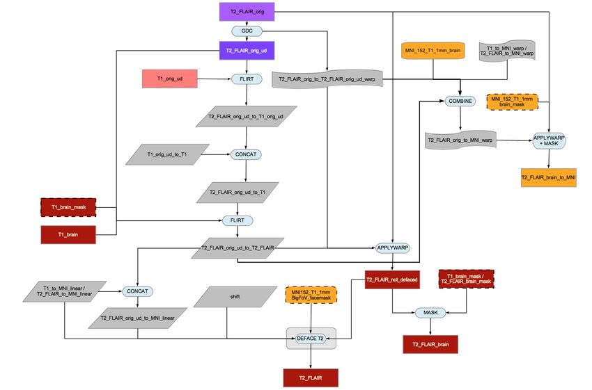
1     Introduction

This documentation describes the brain imaging component of the UK Biobank prospective epidemiological study. It provides
details of the acquisition protocols, image processing pipeline, image data files and derived measures (IDPs - imaging-derived
phenotypes) of brain structure and function.

Researchers wanting to avoid reading the full technical detail relating to the imaging and image processing may wish to concentrate
on Sections 1 and 4.

1.1     UK Biobank - background

UK Biobank is a prospective cohort study of over 500,000 individuals from across the United Kingdom. Participants, aged between
40 and 69, were invited to one of 22 centres across the UK between 2006 and 2010. Blood, urine and saliva samples were collected,
physical measurements were taken, and each individual answered an extensive questionnaire focused on questions of health and
lifestyle. The resource will provide a picture of how the health of the UK population develops over many years and it will enable
researchers to improve the diagnosis and treatment of common diseases.

UK Biobank has collected genetic data on every participant. It has also begun to invite back some of the original participants for
brain, heart and body imaging. It is the brain imaging that is the subject of this document.

The UK Biobank resource is open to the research community and it will grow and develop over time. It is a UK Biobank data
access policy that findings that use UK Biobank data should be fed back to UK Biobank and made available to other researchers.
Researchers associated with UK Biobank (such as those helping run the brain imaging) do not get preferential data access and are
not able to carry out their own research with data until it is made available for all researchers.

1.2     Referencing use of Brain Imaging Data

The primary citations for UK Biobank brain imaging are listed below. If you make use of pre-processed image data or the IDPs
(summary measures described below and available from UK Biobank), we would be grateful if this can be made clear in publications;
this will help with ongoing justification to funders for this component of UK Biobank. Appropriate example text might begin with
the following, with additional specific details potentially extracted from this document and the papers referenced below: “Our
study made use of [ imaging-derived phenotypes / pre-processed image data ] generated by an image-processing pipeline
developed and run on behalf of UK Biobank (Alfaro-Almagro, NeuroImage 2018)”. Of course, as is always the case, UK
Biobank Data Access does not require you to add (individual or groupwise) additional co-authorships.

    • Online brain imaging documentation - this document:
      UK Biobank Brain Imaging Documentation.
      Stephen Smith, Fidel Alfaro Almagro and Karla Miller.
      biobank.ctsu.ox.ac.uk/crystal/docs/brain_mri.pdf

    • Primary citation for brain imaging in UK Biobank:
      Multimodal population brain imaging in the UK Biobank prospective epidemiological study.
      K.L. Miller, F. Alfaro-Almagro, N.K. Bangerter, D.L. Thomas, E. Yacoub, J. Xu, A.J. Bartsch, S. Jbabdi, S.N. Sotiropoulos,
      J.L.R. Andersson, L. Griffanti, G. Douaud, T.W. Okell, P. Weale, I. Dragonu, S. Garratt, S. Hudson, R. Collins, M. Jenkinson,
      P.M. Matthews, and S.M. Smith.
      Nature Neuroscience, 19(11):1523–1536, 2016.

    • Primary citation for the brain imaging processing pipeline and IDPs:
      Image processing and Quality Control for the first 10,000 brain imaging datasets from UK Biobank.
      F. Alfaro-Almagro, M. Jenkinson, N.K. Bangerter, J.L.R. Andersson, L. Griffanti, G. Douaud, S.N. Sotiropoulos, S. Jbabdi,
      M. Hernandez-Fernandez, E. Valee, D. Vidaurre, M. Webster, P. McCarthy, C. Rorden, A. Daducci, D.C. Alexander, H.

                                                                 4
Zhang, I. Dragonu, P.M. Matthews, K.L. Miller and S.M. Smith.
      NeuroImage 166(400–424), 2018.

1.3    UK Biobank Brain Imaging

Because of the very large numbers of study participants, the entire brain imaging protocol has to be completed within 35 min-
utes. Much effort has been made to optimise image quality given this strict limitation, and to achieve a suitable balance (of
time/quality/robustness) between the different modalities acquired. To date the brain imaging data acquisition includes 6 modal-
ities, covering structural, diffusion and functional imaging, with the order below reflecting the actual acquisition ordering:

   • T1 A T1-weighted structural image. T1-weighted imaging is a structural technique with high-resolution depiction of
     brain anatomy, having strong contrast between grey and white matter, reflecting differences in the interaction of water with
     surrounding tissues (tissue T1 relaxation times). This modality provides IDPs primarily relating to volumes of brain tissues
     and structures. It is also critical for calculations of cross-subject and cross-modality alignments, needed in order to process
     all other brain modalities.

   • rfMRI Resting-state functional MRI timeseries data. Resting-state functional MRI measures changes in blood oxygenation
     associated with intrinsic brain activity (i.e., in the absence of an explicit task or sensory stimulus). Derived IDPs estimate
     the apparent connectivity between pairs of brain regions, as reflected in the presence of spontaneous co-fluctuations in signal
     (i.e., the appearance of a connection based on co-activity, as opposed to a structural tract from dMRI). Other IDPs reflect
     the amplitude of spontaneous fluctuation within each region.

   • tfMRI Task functional MRI timeseries data. Task functional MRI uses the same measurement technique as resting-state
     fMRI, while the subject performs a particular task or experiences a sensory stimulus. Derived IDPs relate to the strength of
     response to the specific task (or a specific component of a more complex cognitive process) within a given anatomical brain
     region. The task used in Biobank was chosen to engage a range of high-level cognitive systems.

   • T2_FLAIR A T2-weighted FLAIR structural image. T2-weighted imaging is a structural technique with contrast dominated
     by signal decay from interactions between water molecules (T2 relaxation times). Image intensity is primarily related to
     pathology, with relatively subtle signal differences between grey and white matter. T2 images depict alterations to tissue
     compartments typically associated with pathology (e.g., white matter lesions).

   • dMRI Diffusion MRI. Diffusion-weighted imaging is a structural technique that measures the ability of water molecules to
     move within their local tissue environment. Water diffusion is measured along a range of orientations, providing two types
     of IDPs. Local (voxel-wise) estimates of diffusion properties reflect the integrity of microstructural tissue compartments
     (e.g., diffusion tensor estimates). Long-range estimates based on tract-tracing (tractography) reflect structural connectivity
     between pairs of brain regions.

   • SWI Susceptibility-weighted imaging. Susceptibility-weighted imaging is a structural technique that is sensitive to mag-
     netized tissue constituents (magnetic susceptibility). Data from one scan (including phase and magnitude images from two
     echo times) can be processed in multiple ways to reflect venous vasculature, microbleeds or aspects of microstructure (e.g.,
     iron, calcium and myelin).

In addition to releasing raw data, an initial image processing pipeline has been run that has generated processed versions of the data,
using publicly available image processing tools, primarily taken from FSL (the FMRIB Software Library [Jenkinson et al., 2012]) and
more recently also FreeSurfer [Dale et al., 1999]. For example, the T1 structural image has been processed to remove non-brain
parts of the image, and to segment the brain image into different tissue types. The pipeline has also been used to generate several
QC (quality control) measures.

For most of the brain imaging modalities, the pipeline has also been used to generate many IDPs (image-derived phenotypes).
These numerical pipeline outputs aim to be objective quantifications of different aspects of brain structure and function. IDPs
range from simple gross measures, such as total brain volume, to very specific detailed measures, such as average functional
connectivity between two specific brain regions. The goal is for IDPs to be useful summary measures derived from the imaging

                                                                  5
data, that can be used in analyses to relate to other non-imaging variables in UK Biobank, such as health outcome measures. Each
IDP is presented as a separate data field within the UK Biobank showcase http://www.ukbiobank.ac.uk/data-showcase.

Over the coming months/years, the goal is to expand the analysis pipeline, including state of the art processing from a broader
range of methods/models and software toolkits, where this will increase the quality, robustness and scope of processing applied and
IDPs generated. One high priority is to adapt the FreeSurfer / Human Connectome Project pipelines to achieve cortical surface
modelling (FreeSurfer cortical structural modelling has now been incorporated and released; HCP-style cortical modelling of fMRI
data will hopefully be available later in 2020).

Some image data quality control (a combination of manual and automated checking) has taken place as part of the data processing;
for example, IDPs are not generated for datasets that have been identified as being incomplete or very badly affected by artefacts.
However, UK Biobank is committed to making available to researchers all imaging data acquired (see below for more details),
and not just imaging datasets judged to be of very high quality. This is in part because different researchers may have different
definitions of “acceptable quality”, and also because some researchers may want to develop their own processing pipelines to
detect/correct image data quality problems. Therefore for any research carried out on the basis of the image data and IDPs, it is
important to verify the quality of the datasets used in that research.

An email discussion list has been setup for researchers wanting to discuss any aspects of the UK Biobank brain imaging protocols,
data and analysis: https://www.jiscmail.ac.uk/cgi-bin/webadmin?A0=UKB-NEUROIMAGING

1.4    What’s new in documentation / data-release versions
  • v1.7 January 2020. Added 18k new subjects, plus 1.5k second-scan subjects. Added new confound variables. 40k subjects
    total.

  • v1.6 May 2019. Added FreeSurfer processing and IDPs. 22k subjects.

  • v1.5 August 2018. General documentation update, including new information about imaging confounds. 22k subjects.

  • v1.4 December 2017. Minor documentation update. 15k subjects.

  • v1.3 January 2017. Added white matter lesion segmentation and associated IDP. Added cortical ROIs’ grey matter volume
    IDPs. 10k subjects.

  • v1.2 August 2016. Added resting-state fMRI fluctuation amplitude IDPs. 5k subjects.

  • v1.1 January 2016. Minor documentation changes. 5k subjects.

  • v1.0 October 2015. Original data release and documentation. 5k subjects.

                                                                6
2     Image acquisition protocols

This section describes the imaging hardware and acquisition protocols (in the order that the different modalities are
acquired within the imaging session).   The full protocol PDF (as auto-generated by the scanner) is provided at
http://biobank.ctsu.ox.ac.uk/crystal/refer.cgi?id=2367; the most important protocol parameters are given below.

2.1    Brain imaging hardware

The scanner is a standard Siemens Skyra 3T running VD13A SP4 (as of October 2015), with a standard Siemens 32-channel RF
receive head coil.

At this point all released data is from a single scanner dedicated to UK Biobank imaging, in Cheadle Manchester. In 2017 two
further identical centres (in Newcastle and Reading) will begin scanning.

2.2    Echo-planar imaging

The EPI-based acquisitions (dMRI, rfMRI and tfMRI) utilize simultaneous multi-slice (multiband) acceleration
[Larkman et al., 2001, Moeller et al., 2010]. Biobank uses pulse sequences and reconstruction code from the Center for
Magnetic Resonance Research (CMRR), University of Minnesota https://www.cmrr.umn.edu/multiband. These developments
were partially generated as part of the Human Connectome Project (HCP, NIH grant 1U54MH091657), as described in
[Ugurbil et al., 2013].

The fMRI data and primary dMRI data are all acquired with AP (anterior-posterior) phase encoding direction.

Distortion correction of EPI requires an estimate of the static field map. This fieldmap is derived from pairs of spin-echo EPI
acquisitions with opposite phase encoding directions, acquired as part of the dMRI dataset; in addition to the primary dMRI data,
3 b=0 images are acquired with reversed phase encoding for later fieldmap estimation (along with 3 b=0 images with standard
phase encoding). The estimated fieldmap is used for distortion correction in both the dMRI and fMRI datasets. This aproach was
found to have similar accuracy to separate fieldmap acquisitions in much shorter time and with greater robustness against head
motion.

2.3    Setup, shimming

Duration: 2 minutes

It is critical to achieve maximally consistent spatial coverage of scans in the presence of differences in subject positioning and head
size. For each scan, the field-of-view is automatically determined based on Siemens’ auto-align software, which aligns a scout scan
to an atlas. In the infrequent situation where auto-align failed, alignment was set by the radiographer.

T1 and T2 structurals are acquired using straight sagittal orientation (i.e., with the field-of-view aligned to the scanner axes).
fMRI (task and resting-state), dMRI and SWI utilise slice angling to minimise the superior-inferior field-of-view, thus optimising
volume acquisition speed. Using the population brain size and shape results from [Mennes et al., 2014], imaging matrix is angled
such that the front of the brain is tilted down (relative to the imaging matrix) by 16◦ , with respect to the AC-PC line.

Shim field accuracy is critical for data quality, and was found to be suboptimal when using default settings on the MRI scanner,
particularly for the simultaneous multi-slice EPI acquisitions. Initially, shim quality was improved by manually iterating the shimming
process 3 times; this process which was later replaced by a single shim using a reduced shimming field-of-view, thereby improving
resolution of the acquired field map. The scans are prescribed to avoid any subsequent re-shimming during the entire protocol.

                                                                  7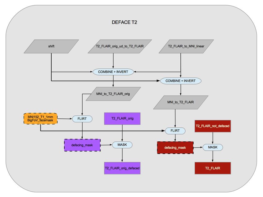
2.4    T1-weighted structural imaging

Resolution: 1x1x1 mm
Field-of-view: 208x256x256 matrix
Duration: 5 minutes
3D MPRAGE, sagittal, in-plane acceleration iPAT=2, prescan-normalise

The superior-inferior field-of-view is large (256mm), at little cost, in order to include reasonable amounts of neck/mouth, as those
areas will be of interest to some researchers.

2.5    Resting-state functional MRI

Resolution: 2.4x2.4x2.4 mm
Field-of-view: 88x88x64 matrix
Duration: 6 minutes (490 timepoints)
TR: 0.735 s
TE: 39ms
GE-EPI with x8 multislice acceleration, no iPAT, flip angle 52◦ , fat saturation

As implemented in the CMRR multiband acquisition, a separate “single-band reference scan” is also acquired. This has the same
geometry (including EPI distortion) as the timeseries data, but has higher between-tissue contrast to noise, and is used as the
reference scan in head motion correction and alignment to other modalities.

2.6    Task functional MRI

As for rfMRI, except:
Duration: 4 minutes (332 timepoints)

The task is the Hariri faces/shapes “emotion” task [Hariri et al., 2002, Barch et al., 2013], as implemented in the HCP, but with
shorter overall duration and hence fewer total stimulus block repeats. The participants are presented with blocks of trials and
asked to decide either which of two faces presented on the bottom of the screen match the face at the top of the screen, or which
of two shapes presented at the bottom of the screen match the shape at the top of the screen. The faces have either angry or
fearful expressions.

The ePrime script that controls the video presented to the participant is derived from the one used by the HCP, and is available
at http://biobank.ctsu.ox.ac.uk/crystal/refer.cgi?id=1462.

2.7    T2-weighted FLAIR structural imaging

Resolution: 1.05x1x1 mm
Field-of-view: 192x256x256 matrix
Duration: 6 minutes
3D SPACE, sagittal, in-plane acceleration iPAT=2, partial Fourier = 7/8, fat saturation, elliptical k-space scanning, prescan-
normalise

After early piloting, a standard T2/PD-weighted acquisition was dropped due to a combination of factors such as overall value and
timing practicalities. However a T2-weighted FLAIR image is acquired, which is generally of good quality and which shows strong
contrast for white matter hyperintensities.

                                                                 8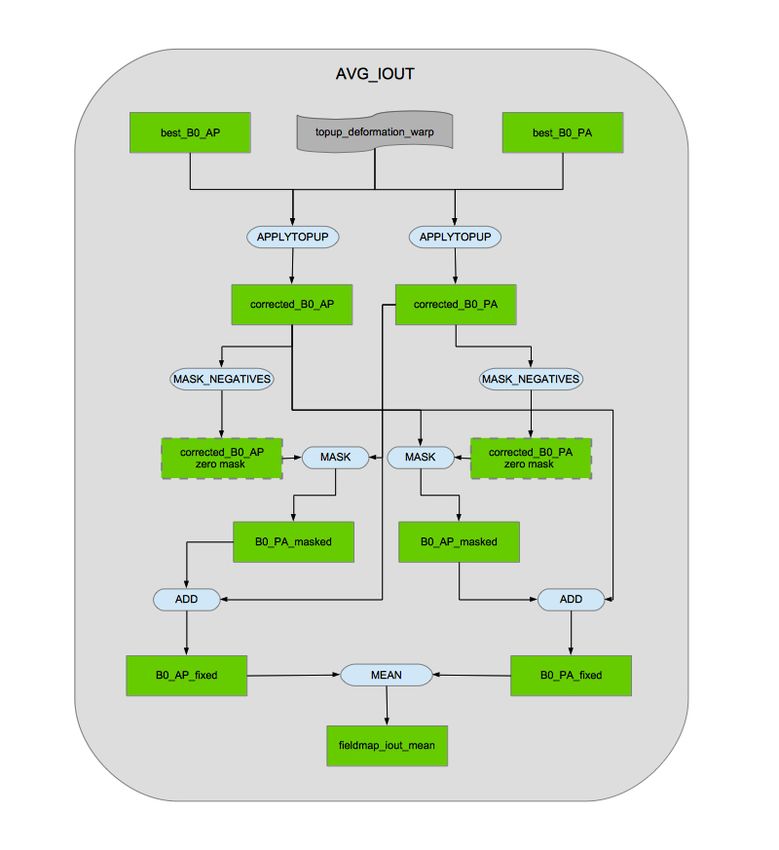
2.8      Diffusion imaging

Resolution: 2x2x2 mm
Field-of-view: 104x104x72 matrix
Duration: 7 minutes (including 36 seconds phase-encoding reversed data)
5x b=0 (+3x b=0 blip-reversed), 50x b=1000 s/mm2 , 50x b=2000 s/mm2
Gradient timings: δ=21.4 ms, ∆=45.5 ms; Spoiler b-value = 3.3 s/mm2
SE-EPI with x3 multislice acceleration, no iPAT, fat saturation

For the two diffusion-weighted shells, 50 distinct diffusion-encoding directions were acquired (and all 100 directions are distinct).
The diffusion prepraration is a standard (“monopolar”) Stejskal-Tanner pulse sequence. This enables higher SNR due to a shorter
echo time (TE=92ms) than than a twice-refocused (“bipolar”) sequence. This improvement comes at the expense of stronger
eddy current distortions, which are removed in the image processing pipeline.

2.9      Susceptibility-weighted structural imaging

Resolution: 0.8x0.8x3 mm
Field-of-view: 256x288x48 matrix
Duration: 2.5 minutes
Two echos, TE=9.42,20 ms
3D, axial, in-plane acceleration iPAT=2, partial Fourier = 7/8, prescan-normalise

To date the magnitude and phase images have been saved for each RF coil and echo time separately.

2.10      Compatibility across different phases of imaging

Ideally the imaging protocol will stay fixed over time. However, early improvements in the dMRI and T2_FLAIR protocols were
found to be very valuable, resulting in significant enough data improvements to outweigh the priority of holding things perfectly
constant (and taking into account the relatively small numbers of datasets affected). This change was made at the start of protocol
“Phase 3”; the different phases are described in detail below. A variable available in the UK Biobank database (Acquisition protocol
phase) specifies which protocol phase (currently from 1 to 5) was used for a given subject.

2.10.1    Protocol Phase 1

Only 11 datasets were acquired within this initial phase, after which several major improvements were made in the protocol. None
of these datasets were processed with the image processing pipeline to generate IDPs or processed imaging data.

2.10.2    Protocol Phase 2 (compared with Phase 3 and later)

Approximately 500 datasets were acquired with a protocol which, for dMRI and T2_FLAIR, are incompatible with later phases
(i.e., are different from what is shown in the Siemens protocol PDF linked above). These differences are now described.

The Phase 2 T2_FLAIR scans did not use elliptical k-space coverage (which was used in later scans to reduce acquisition time
with no significant loss in image quality), and used 6/8 partial-Fourier (instead of the later 7/8 partial-Fourier, a change which
reduced image blurring in later scans with a small time penalty).

The Phase 2 dMRI scans used “bipolar” (twice-refocused spin echo) diffusion encoding, instead of the “monopolar” (Stejskal-
Tanner single spin echo) approach used later. Recent advances in post-processing are able to remove the greater image distortions
incurred by monopolar encoding, allowing a reduction in echo time from 112ms to 92ms, providing a substantial increase in SNR
and reducing the TR from 4.06s to 3.6s, providing a large reduction in scan time. Other (more minor) differences in Phase 2 dMRI

                                                                 9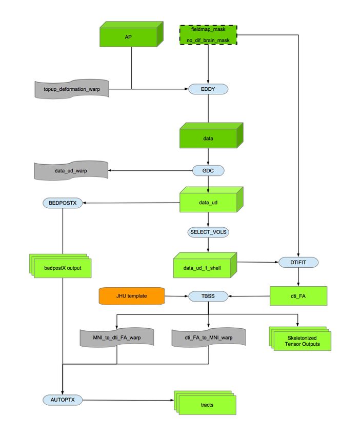
scans (compared with Phase 3) are: one fewer diffusion encoding direction per shell, a larger flip angle (93/180 instead of the later
78/160) and a greater number of blip-reversed b=0 images (5 instead of the later 3).

As described in more detail below, for these early “incompatible” scans, the raw T2_FLAIR and dMRI NIFTI images are available
via the UK Biobank database, but have not been used in the full image processing pipeline, and do not have IDPs computed (as
these would likely be incompatible with those generated later).

One final minor difference in the Phase 2 scans, which does not present incompatibility problems, is that the rfMRI and tfMRI
protocols had additional timepoints (approximately 30s) compared with later scans.

2.10.3   Protocol Phase 4 (compared with Phase 3)

No significant changes were made between Phase 3 and 4. Three superfluous b=0 scans were removed. The T2_FLAIR was
moved within the protocol to run after the fMRI scans. A new auto-shimming approach was put in place, with a reduced shimming
field-of-view and fewer shim iterations; this saved time and was evaluated to result in very similar shimming quality. A small
cross-hair was added to the video display, for subjects to focus on (except during tfMRI).

2.10.4   Protocol Phase 5

No significant changes; CMRR multiband software was upgraded to v12 (R012b).

2.10.5   Protocol Phase 6

No significant changes; CMRR multiband software was upgraded to R014.

2.10.6   Protocol Phase 7

No significant changes; CMRR multiband software was upgraded to R015.

2.10.7   Protocol Phase 8

No significant changes; Siemens scanner software was upgraded with service-pack SP7.

                                                                 10
3 Image processing pipeline
The full set of image analysis pipeline scripts are available from https://www.fmrib.ox.ac.uk/ukbiobank/ - at present the
scripts primarily call tools from FSL and FreeSurfer.
3.1 Reconstruction of real-space data from k-space complex data
Images in the “real space” domain were reconstructed from the complex k-space domain in which data are collected. Unless
otherwise specified, all images are signal magnitude.
Standard Siemens on-scanner conversion of complex multi-coil data was carried out for the T1 and T2_FLAIR data.
Image reconstruction for the simultaneous multi-slice EPI data (dMRI, rfMRI, tfMRI) was carried out using reconstruction software
supplied by CMRR (available from the CMRR web site listed above).
SWI data has, to date, been saved as coil-separated real-space complex data, as it has not yet been possible to carry out appropriate
multi-coil combination on the scanner for accurate reconstruction of phase images. This is expected to change in the near future.
3.2 Raw DICOM data conversion to NIFTI and download options
All real-space DICOM image files are converted to NIFTI format using Chris Rorden’s conversion tool dcm2niix
https://github.com/rordenlab/dcm2niix. This tool also generates the diffusion-encoding b values and vectors files.
Image data is available from UK Biobank in both DICOM and (separately) NIFTI formats. Both forms include the raw (non-
processed) data, the only differences being that the NIFTI-version T1/T2 structural images are defaced for subject anonymity (as
described below), and the full multi-coil (pre-combination) SWI data is only available in the DICOM downloads. An individual
zipfile download is for one modality from one subject for one data format (DICOM or NIFTI).
The NIFTI versions are the recommended option, partly because for each modality a small number of simply and consistently named
images are provided (e.g., T1, rfMRI), as opposed to thousands of separate DICOM files (with complex naming conventions).
Also, the NIFTI downloads, while overall only being 40% larger than pure-raw DICOM downloads, include not just the the raw
images, but also images output by the processing pipeline, for example after gradient distortion correction (for all modalities), and
correction for eddy currents and head motion (dMRI data), and artefact removal (rfMRI data).
3.3 Image anonymisation and raw DICOM data access
In order to protect study participant anonymity, the high resolution structural images (T1 and T2) are “defaced”. This involves
setting voxels in the general regions of the face and ears to zero. This is achieved by estimating a linear transformation between
the original data and a standard co-ordinate system (an expanded MNI152 template space), and back-projecting standard-space
regions-of-interest into the native data, to allow for masking-out of the face/ears. Testing for overlap between (non-defaced) brain
masks and the defacing masks shows only 8 subjects with any overlap at all, and all qualitatively show virtually no loss of brain
voxels.
Hence in the NIFTI-format data released by UK Biobank, for the T1 and T2 data, only defaced versions are available (to protect
anonymity of study participants). This matches common practice such as that in the HCP. The raw, non-defaced DICOM T1 and
T2 data is classified as sensitive by UK Biobank; researchers requiring raw DICOM non-defaced T1/T2 data should contact UK
Biobank to discuss this further.
113.4 Data/Folder file organisation
For each subject, the raw and processed imaging data files are organised into subfolders according to the different modalities (and
described in more detail for each modality below).
When raw data is corrupted, missing or otherwise unusable, it is moved into a subfolder (inside the given modality’s folder) named
unusable, and not processed any further (apart from defacing applied to the raw T1 and T2_FLAIR). This “unusable” data is
included in the Biobank database, because some researchers may be interested in working with this data, for example, to develop
new methods for detecting or even possibly correcting such data.
The evaluation of the T1 data for “usability” includes a rough manual review of all T1s (supplemented by a beta-version auto-QC
approach) [Alfaro-Almagro et al., 2018]. Where a T1 is considered to have a serious problem it has been moved into the “unusable”
subfolder as described above. This is for datasets where the issue is considered serious enough that the pipeline is unlikely to run
well - which could be imaging artefacts/problems or very gross pathologies. More subtle pathologies that are subtle enough that
we expect the pipeline to run OK are not treated as “unusable” in this way.
In the case of unusable T1 data, all other modalities’ raw imaging data are also considered unusable (because the pipeline cannot
function without a usable T1). However, as with the T1 data, all such raw data is still available for download in the NIFTI packages
(but without the pipeline processing applied).
In the case of the incompatible (Phase 2) dMRI and T2_FLAIR data (see above for protocol incompatibilities), these also are
not processed with the image processing pipeline, but the raw data are moved to an incompatible folder, and available for
download. For example, some researchers may wish to investigate the possibility of developing analyses which can handle the
protocol incompatibilities.
3.5 Gradient distortion correction
Full 3D gradient distortion correction (GDC) is not available on the scanner for EPI data, and so all GDC is applied within
the image analysis pipelines. Tools developed by the FreeSurfer and HCP teams are used for applying the correction, available
at https://github.com/Washington-University/Pipelines. To run these tools also requires a proprietary data file from
Siemens which describes the gradient nonlinearities (coeff.grad).
3.6 T1 processing
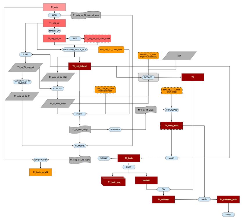
The raw original (defaced) T1-weighted structural image and other T1-derived pipeline outputs are in the folder T1.
The full FoV (field-of-view) raw T1 image, after defacing, is T1_orig_defaced. Apart from the defacing (and the fact that bias
field has already been reduced via the on-scanner “pre-scan normalise” option), this is the raw T1 structural data, without any
further processing such as gradient distortion correction.
The FoV is then cut down to reduce the amount of non-brain tissue (primarily blank space above the head and tissues below the
brain), and GDC applied. Tools utilised to achieve this robustly include BET (Brain Extraction Tool [Smith, 2002]) and FLIRT
(FMRIB’s Linear Image Regsitration Tool [Jenkinson and Smith, 2001, Jenkinson et al., 2002]), in conjunction with the MNI152
“nonlinear 6th generation” standard-space T1 template http://www.bic.mni.mcgill.ca/ServicesAtlases/ICBM152NLin6.
This results in the reduced-FoV T1 head image T1.
The data is now nonlinearly warped to MNI152 space using FNIRT (FMRIB’s Nonlinear Image Registration
Tool [Andersson et al., 2007b, Andersson et al., 2007a]), resulting in the warp transform file transforms/T1_to_MNI_warp_coef.
A standard-space brain mask is then back-transformed into the space of the T1 (generating T1_brain_mask), and applied to the
T1 image to generate a brain-extracted T1, T1_brain.
Next, tissue-type segmentation is applied using FAST (FMRIB’s Automated Segmentation Tool [Zhang et al., 2001]), with
outputs in subfolder T1_fast. This provides a hard segmentation into CSF (cerebrospinal fluid), grey matter and white
12matter (T1_brain_seg), as well as partial-volume images for each tissue type (T1_brain_pve_0, T1_brain_pve_1 and
T1_brain_pve_2, respectively). This processing is also used to generate a fully bias-field-corrected version of the brain-extracted
T1: T1_unbiased_brain.
These data are then used to carry out a SIENAX-style analysis (Structural Image Evaluation, using Normalisation, of Atrophy:
Cross-sectional [Smith et al., 2002]). The external surface of the skull is estimated from the T1, and used to normalise brain tissue
volumes for head size (compared with the MNI152 template). Volumes of different tissue types and total brain volume, both
normalised for head size, and not normalised, are generated as IDPs and accessible from the UK Biobank database.
The FAST grey matter segmentation is also used to generate a further 139 IDPs, by summing the grey matter partial volume
estimates within 139 ROIs. These ROIs are defined in MNI152 space, combining parcellations from several atlases: the Harvard-
Oxford cortical and subcortical atlases https://fsl.fmrib.ox.ac.uk/fsl/fslwiki/Atlases and the Diedrichsen cerebellar
atlas http://www.diedrichsenlab.org/imaging/propatlas.htm . The previously estimated warp field (taking the subject’s
data into standard space) is inverted and applied to the ROIs, to generate a version of the ROIs in native space, for masking onto
the segmentation.
Subcortical structures (shapes and volumes) are modelled using FIRST (FMRIB’s Integrated Registration and Segmentation
Tool [Patenaude et al., 2011]). The shape and volume outputs for 15 subcortical structures (in files *.bvars and *.vtk -
see http://fsl.fmrib.ox.ac.uk/fsl/fslwiki/FIRST/UserGuide) are stored in the T1_first subfolder. A single summary
image, with a distinct integer value coding for each structure, is T1_first_all_fast_firstseg. The volumes of the different
structures are saved as IDPs in the Biobank database.
The T1 images are also processed with FreeSurfer tools. Where available, the T2_FLAIR is used in conjunction with the T1 to
achieve more accurate cortical modelling than possible with the T1 only. For some derived measures, such as cortical thickness,
there is a clear bias in thickness estimated when using both inputs vs. just the T1, and so we would recommend either using just
measures derived from analyses using both inputs, or attempting deconfounding. The variable indicating this information is at
http://biobank.ndph.ox.ac.uk/showcase/field.cgi?id=26500 in the UK Biobank database. FreeSurfer outputs (images,
surface files and summary outputs) are available for download in a single zipfile per subject. These live in the FreeSurfer subfolder.
The primary FreeSurfer modelling is of the cortical surface [Dale et al., 1999, Fischl et al., 1999a, Fischl et al., 1999b]. Sur-
face templates are used to extract IDPs relating to standard atlas regions’ surface area, volume and mean cortical thick-
ness [Fischl et al., 2004, Desikan et al., 2006]. Subcortical regions are extracted using FreeSurfer’s aseg tool [Fischl et al., 2002],
and also further sub-segmentation of some subcortical regions is carried out [Iglesias et al., 2015], resulting in additional IDPs.
3.7 T2_FLAIR processing
The original (defaced) T2-weighted structural image and other pipeline outputs are in folder T2_FLAIR.
The full FoV T2 image, after defacing, is T2_FLAIR_orig_defaced.
The T2 image is linearly aligned to the T1 using FLIRT, and the resulting transform is then combined with various trans-
forms derived from the T1, in order to transform the T2 directly from the original space into both the individual subject’s T1
space and MNI standard space. By analogy with the T1-related images described above, this results in images T2_FLAIR and
T2_FLAIR_brain, and a bias-corrected version of the latter T2_FLAIR_brain_unbiased (these being in the space of the T1), as
well as T2_FLAIR_brain_to_MNI (MNI-space version).
The total volume of white-matter hyperintensities (WMHs, or white matter lesions) is estimated to generate an additional IDP.
This is primarily utilising the T2_FLAIR data, but also the T1 data; this lesion segmentation is automatically carried out using
the BIANCA tool[Griffanti et al., 2016].
133.8 SWI processing
The original SWI data and other pipeline outputs are in folder SWI. This data can provide a range of maps with distinct features
related to magnetic susceptibility. Phase images have the potential to be used for quantitative susceptibility mapping, magnitude
data can be used to calculate T2* relaxation rates and both magnitude and phase are used for generating venograms (see below)
and for visualizing hemosiderin in microbleeds.
Combining phase images across coils requires care due to anomolous phase transitions in regions of focal signal dropout for a
given coil. Currently, all coil channels are saved separately to enable combination of phase images in post-processing. Each coil
channel phase image is first high-pass filtered to remove low-frequency phase variations (including both coil phase profiles and field
distortion from bulk shape). A combined complex image is generated as the sum of the complex data from each coil (unfiltered
magnitude and filtered phase), and the final phase image (filtered_phase) is the phase of this summation. Careful inspection
of a small number of subjects found no anomolous phase transitions from individual channels in the final combined image.
Venograms (SWI) were calculated using an established reconstruction [Haacke et al., 2004], in which magnitude images are mul-
tiplied by a further filtration of the phase data to enhance the appearance of veins. The phase image is first thresholded (such
that only paramagnetic susceptibility is non-unitary) and then taken to the fourth power to enhance contrast in veins. The chosen
power represents a tradeoff between venous-tissue contrast and noise in the phase data.
R2* values were calculated from the magnitude data. First, a single magnitude image is calculated for each of the two echo times
TE1 and TE2. This is calculated by taking the square of the magnitude image from each individual coil channel, summing across
channels, and then taking the square root (typically referred to as “sum-of-squares” combination). The log of the ratio of these
two echo time images (SOS_TE1 and SOS_TE2) was calculated, and scaled by the echo time difference, to give the R2*. T2* is
calculated as the inverse of R2*. The T2* image is then spatially filtered (3x3x1 median filtering followed by limited dilation to
fill missing data holes) to reduce noise (resulting in T2star), and transformed into the space of the T1 (via registration of the
bias-field-normalised magnitude image SWI_TOTAL_MAG), the resulting image being T2star_to_T1.
3.9 B0 fieldmap processing
The B0 fieldmap-related pipeline outputs are in folder fieldmap (although these are derived primarily from the dMRI data).
All b=0 dMRI images with opposite phase-encoding direction (anterior-posterior (AP) and posterior-anterior (PA)) are anal-
ysed, to identify the highest-quality pair of AP and PA images. This optimal AP/PA pair is then fed into Topup
http://fsl.fmrib.ox.ac.uk/fsl/fslwiki/TOPUP [Andersson et al., 2003] in order to estimate the B0 fieldmap and asso-
ciated dMRI EPI distortions. GDC is then applied.
The EPI distortion information needed by the remaining dMRI processing is saved in files fieldmap_out_fieldcoef.nii.gz and
fieldmap_out_movpar.txt.
The magnitude image is then linearly aligned to the T1, for later use in unwarping the fMRI data; the resulting transformation is
the applied to the fieldmap, resulting in the T1-space fieldmap fieldmap_fout_to_T1_brain_rad.
3.10 dMRI processing
The original dMRI data and processing pipeline outputs are in folder dMRI. The raw data is in folder dMRI/raw, which contains
the primary data used for diffusion analyses (AP), along with associated b value and vector text files, and the 3 b=0 phase-reversed
images (PA).
First the data is corrected for eddy currents and head motion, and has outlier-slices (individual slices in the 4D
data) corrected, using the Eddy tool http://fsl.fmrib.ox.ac.uk/fsl/fslwiki/EDDY [Andersson and Sotiropoulos, 2015,
Andersson and Sotiropoulos, 2016]. GDC is then applied, resulting in the 4D output file dMRI/data_ud.
This is then fed into two complementary analyses, one based on tract-skeleton processing, and the other based on a richer
14modelling of within-voxel tract structure, followed by probabilistic tractography analysis (BEDPOSTx / PROBTRACKx). Both
analysis streams then report a range of dMRI-derived measures within different tract regions: A) measures derived from diffusion-
tensor modelling, and B) measures derived from microstructural model fitting. Outputs from both these modellings are in the
dMRI subfolder.
The b=1000 shell (50 directions) is fed into the diffusion-tensor-imaging (DTI) fitting tool DTIFIT, creating DTI outputs such as
fractional anisotropy dMRI/dti_FA, tensor mode dMRI/dti_MO and mean diffusivity dMRI/dti_MD.
In addition to the DTI fitting, the dMRI data is fed into NODDI (Neurite Orientation Dispersion and Density Imaging) modelling,
using the AMICO (Accelerated Microstructure Imaging via Convex Optimization) tool https://github.com/daducci/AMICO
[Zhang et al., 2012, Daducci et al., 2015]. This aims to generate meaningful voxelwise microstructural parameters, including ICVF
(intra-cellular volume fraction - an index of white matter neurite density), ISOVF (isotropic or free water volume fraction) and OD
(orientation dispersion index, a measure of within-voxel tract disorganisation).
3.10.1 TBSS-style analysis
The DTI FA image is then fed into TBSS (Tract-Based Spatial Statistics [Smith et al., 2006]), which aligns the FA image
onto a standard-space white-matter skeleton, with alignment improved over the original TBSS skeleton-projection method-
ology through utilisation of a high-dimensional FNIRT-based warping [de Groot et al., 2013]. The resulting standard-space
warp (TBSS/FA/dti_FA_to_MNI_warp) is applied to all other DTI/NODDI outputs. The final skeleton-space outputs are in
TBSS/stats/all_*_skeletonised, where * represents each of the DTI and NODDI outputs (FA, etc). For each of the
DTI/NODDI outputs, these skeletonised images are averaged across a set of 48 standard-space tract masks defined by the
group of Susumi Mori at Johns Hopkins University [Mori et al., 2005, Wakana et al., 2007], similar to the processing applied in
the ENIGMA project http://enigma.ini.usc.edu/protocols/dti-protocols.
3.10.2 Probabilistic-tractography-based analysis
Separately from the tensor/TBSS analysis, the Eddy output data is also fed into tractography-based analysis. This begins
with within-voxel modelling of multi-fibre tract orientation structure via the BEDPOSTx tool (Bayesian Estimation of Diffu-
sion Parameters Obtained using Sampling Techniques) http://fsl.fmrib.ox.ac.uk/fsl/fslwiki/FDT/UserGuide followed
by probabilistic tractography (with crossing fibre modelling) using PROBTRACKx [Behrens et al., 2003, Behrens et al., 2007,
Jbabdi et al., 2012]. The BEDPOSTx outputs are in folder dMRI.bedpostX; for example, the posterior mean fractional
voxel occupancy for the principle fibre is mean_f1samples and the posterior mean direction of this fibre is dyads1.
The BEDPOSTx outputs are suitable for running tractography from any (voxel or region) seeding; the pipeline has al-
ready automatically mapped a set of 27 major tracts using standard-space start/stop ROI masks defined by AutoPtx
http://fsl.fmrib.ox.ac.uk/fsl/fslwiki/AutoPtx [de Groot et al., 2013]. Although the Eddy and BEDPOSTx outputs are
in the space and resolution of the (GDC-unwarped) native diffusion data space, the nonlinear transformation between this space
and 1mm MNI standard space (as estimated by TBSS above) is used to create tractography results in 1mm standard space.
PROBTRACKx outputs are in autoptx_preproc/tracts. For each tract, and for each DTI/NODDI output image type, an IDP
is generated - the weighted-mean value of the DTI/NODDI parameter within the tract (the weighting being determined by the
tractography output).
3.11 rfMRI processing
The rfMRI data and processing outputs are in folder fMRI; the raw (original) timeseries data is rfMRI and the single-band (single
timepoint) reference scan is rfMRI_SBREF.
The processed rfMRI data is in folder rfMRI.ica. The following pre-processing was applied: motion correction using
MCFLIRT [Jenkinson et al., 2002]; grand-mean intensity normalisation of the entire 4D dataset by a single multiplicative fac-
tor; highpass temporal filtering (Gaussian-weighted least-squares straight line fitting, with sigma=50.0s); EPI unwarping (utilising
the fieldmaps as described above); GDC unwarping. Finally, structured artefacts are removed by ICA+FIX processing (Indepen-
15dent Component Analysis followed by FMRIB’s ICA-based X-noiseifier [Beckmann and Smith, 2004, Salimi-Khorshidi et al., 2014,
Griffanti et al., 2014]). FIX was hand-trained on 40 Biobank rfMRI datasets, and leave-one-out testing showed (mean/median)
99.1/100.0% classification accuracy for non-artefact components and 98.1/98.3% accuracy for artefact components. The final
pre-processed rfMRI timeseries data is filtered_func_data_clean. At this point no lowpass temporal or spatial filtering has
been applied.
The EPI unwarping is a combined step that also includes alignment to the T1, though the unwarped data is written out in native
(unwarped) fMRI space (and the transform to T1 space written out separately). This T1 alignment is carried out by FLIRT, with
a final BBR cost function [Greve and Fischl, 2009]. After the fMRI GDC unwarping, a final FLIRT realignment to T1 is applied,
to take into account any shifts resulting from the GDC unwarping. The previously described transform from T1 space to standard
MNI space is utilised when fMRI data is needed in standard space.
A group-average RSN (resting-state network) analysis was carried out using 4100 datasets. First, each timeseries dataset was
temporally demeaned and had variance normalisation applied according to [Beckmann and Smith, 2004]. Group-PCA output
was generated by MIGP (MELODIC’s Incremental Group-PCA) from all subjects. This comprises the top 1200 weighted spa-
tial eigenvectors from a group-averaged PCA (a very close approximation to concatenating all subjects’ timeseries and then
applying PCA) [Smith et al., 2014]. The MIGP output was fed into group-ICA using FSL’s MELODIC tool [Hyvärinen, 1999,
Beckmann and Smith, 2004], applying spatial-ICA at two different dimensionalities (25 and 100). The dimensionality determines
the number of distinct ICA components; a higher number means that the above-threshold regions within the spatial component maps
will be smaller. The group-ICA spatial maps are available at http://biobank.ctsu.ox.ac.uk/crystal/refer.cgi?id=9028
and also at (with online visualisation) http://www.fmrib.ox.ac.uk/ukbiobank. The sets of ICA maps can be considered as
“parcellations” of (cortical and sub-cortical) grey matter, though they lack some properties often assumed for parcellations - for
example, ICA maps are not binary masks but contain a continuous range of values; they can overlap each other; and a given map
can include multiple spatially separated peaks/regions. Any group-ICA components that are clearly identifiable as artefactual (i.e.,
not neuronally driven) are discarded during the network modelling described below; a text file is supplied with the group-ICA maps,
listing the group-ICA components kept in the final network modelling.
For a given parcellation (group-ICA decomposition of D components), the set of ICA spatial maps was mapped onto each subject’s
rfMRI timeseries data to derive one representative timeseries per ICA component (for these purposes each ICA component is
considered as a network “node”). For each subject, these D timeseries can then be used in network analyses, described below.
This is the first stage in a dual-regression analysis [Filippini et al., 2009]. The single-subject node timeseries are in subfolders
rfMRI_*.dr (where * is the dimensionality).
The node timeseries are then used to estimate subject-specific network-matrices (also referred to as “netmats” or “parcellated
connectomes”). For each subject, the D node-timeseries were fed into network modelling, discarding the clearly artefactual parcels
(nodes), leaving D’ nodes. This results in a D’xD’ matrix of connectivity estimates. Network modelling was carried out using the
FSLNets toolbox http://fsl.fmrib.ox.ac.uk/fsl/fslwiki/FSLNets. Network modelling is applied in two ways: 1. Using full
normalized temporal correlation between every node timeseries and every other. This is a common approach and is very simple, but it
has various practical and interpretational disadvantages including an inability to differentiate between directly connected nodes and
nodes that are only connected via an intermediate node [Smith, 2012]. 2. Using partial temporal correlation between nodes’ time-
series. This aims to estimate direct connection strengths better than achieved by full correlation. To slightly improve the estimates
of partial correlation coefficients, L2 regularization is applied (setting rho=0.5 in the Ridge Regression netmats option in FSLNets).
Netmat values were Gaussianised from Pearson correlation scores (r-values) into z-statistics, including empirical correction for tem-
poral autocorrelation. Group-average netmats are available at http://biobank.ctsu.ox.ac.uk/crystal/refer.cgi?id=9028.
3.12 tfMRI processing
The tfMRI data and processing outputs are in folder fMRI; the raw timeseries data is tfMRI and the single-band (single timepoint)
reference scan is tfMRI_SBREF.
The processed tfMRI data is in folder tfMRI.feat. The same pre-processing and registration was applied as for the rfMRI described
above, except that spatial smoothing (using a Gaussian kernel of FWHM 5mm) was applied before the intensity normalisation,
and no ICA+FIX artefact removal was run. The final pre-processed tfMRI timeseries data is filtered_func_data.
16Task-induced activation modelling was carried out using FEAT (FMRI Expert Analysis Tool); time-series statistical analysis was
carried out using FILM with local autocorrelation correction [Woolrich et al., 2001]. The timings of the blocks of the two task
conditions (shapes and faces) are defined in text files custom_timing_files/ev1.txt and custom_timing_files/ev2.txt.
5 activation contrasts were defined (Shapes, Faces, Shapes+Faces, Shapes-Faces, Faces-Shapes), and an f-contrast also applied
across Shapes and Faces.
The 3 contrasts of most interest are: 1 (Shapes), 2 (Faces) and 5 (Faces-Shapes), with the last of those being of par-
ticular interest with respect to amygdala activation. Group-average activation maps were derived from analysis across all
subjects, and used to define ROIs for generating tfMRI IDPs. Four ROIs were derived; 1 (Shapes group-level fixed-
effect z-statistic, threshoded at Z>120); 2 (Faces group-level fixed-effect z-statistic, threshoded at Z>120); 5 (Faces-Shapes
group-level fixed-effect z-statistic, threshoded at Z>120); 5a (Faces-Shapes group-level fixed-effect z-statistic, threshoded at
Z>120, and further masked by an amygdala-specific mask). The group-average activation maps and ROIs are available
http://biobank.ctsu.ox.ac.uk/crystal/refer.cgi?id=9028.
The Featquery tool was used to extract summary statistics for the 3 main contrasts, for both activation effect size (expressed
as a % signal change relative to the overall-image-mean baseline level) and statistical effect size (z-statistic), with each of these
summarised across the relevant ROI in two ways - median across ROI voxels and 90th percentile across ROI voxels.
Display of the task video and logging of participant responses is carried out by ePrime software, which provides several response log
files from each subject. These are not used in the above analyses (as the timings of the task blocks are fixed and already known,
and the correctness of subject responses are not used in the above analyses), but are available in the UK Biobank database.
174 UK Biobank database (“Showcase”) variables
In addition to the raw and processed “bulk” image data files available from UK Biobank, there are a number of derived numerical
measures available as standalone variables available in the database (i.e., these are summary numbers rather than images). This
includes QC (quality control) measures (such as overall signal-to-noise ratio for individual modalities), IDPs (imaging-derived
phenotypes, such as total brain volume and left hippocampus volume) and other variables that are not QC or IDPs, but which
may be useful as “confound” variables (for example, whether the FreeSurfer processing used the T2_FLAIR image in addition to
the T1). These are now briefly described.
4.1 QC measures
All QC measures are designed such that “higher is worse”.
Several QC measures describe the “discrepancy” (generalised difference) between a given pair of images after they have been aligned
together. Here a poor (large) score could arise either because the quality of the alignment is bad, or because one of the two images
being compared is corrupted in some way. Two such QC measures quantitate the discrepancy between the T1 structural image
and the standard (population average) template image - one after a linear alignment (which cannot correct for the fine-detailed
differences between a given subject and the population average), and the other after a nonlinear alignment (which should achieve
much better correspondence). Related to this, the overall amount of nonlinear warping necessary to achieve a detailed alignment
to the standard template is summarised as one QC measure. Finally, several other QC measures describe the discrepancy between
the T1 image (for a given subject) and each of the other modalities (for that same subject), after linear alignment of the other
modalities to the T1.
Several other QC measures quantitate signal to noise ratio (SNR) in some of the modalities. For the T1, the tissue-type segmen-
tation is used to estimate within-tissue-type noise level (standard deviation), as well as mean intensities for grey and white matter.
These quantities are used to estimate overall image SNR and also CNR (contrast to noise - white-grey mean intensity difference
normalised by noise level). In both cases these measures are inverted before being recorded as QC measures, so that “higher is
worse”. From the preprocessed rfMRI (both before and after artefact removal) and tfMRI timeseries data, similar measures are
calculated, but in this case the “noise” level is the temporal standard deviation. First, voxelwise SNR is calculated, and then the
median (across brain voxels) estimated. This is then inverted for the reported QC measure.
Also from the rfMRI and tfMRI data, the total amount of head motion is summarised as additional QC measures. For each
consecutive pair of timepoints, the mean displacement (averaged across the brain) is estimated, and this is then averaged across
all timepoints.
Finally, from the dMRI data, the total number outlier slices (from all slices in all dMRI volumes) is reported, as output by the
Eddy tool. This is mostly reflective of head motion during the dMRI scan.
4.2 Other confound-regressor variables
In addition to some QC variables, there are several other variables that are likely to be useful as “confound variables” when working
with UKB imaging data. A detailed paper on UKB confounds will be published shortly.
Scanning centre (site)
Data-Field 54 can be used to identify the imaging centre, in case there is any site-specific variability in the imaging (though initial
testing has suggested that there is not large site variability): http://biobank.ctsu.ox.ac.uk/showcase/field.cgi?id=54
For example one might derive a binary indicator confound variable for each site).
Subject’s head size
In general IDPs are not normalised for brain or head size (except for the few SIENAX measures that explicitly state that they
18You can also read