Empirical validation and proof of added value of MUSICA's tropospheric δD remote sensing products
←
→
Page content transcription
If your browser does not render page correctly, please read the page content below
Atmos. Meas. Tech., 8, 483–503, 2015
www.atmos-meas-tech.net/8/483/2015/
doi:10.5194/amt-8-483-2015
© Author(s) 2015. CC Attribution 3.0 License.

Empirical validation and proof of added value of MUSICA’s
tropospheric δD remote sensing products
M. Schneider1 , Y. González2 , C. Dyroff1 , E. Christner1 , A. Wiegele1 , S. Barthlott1 , O. E. García2 , E. Sepúlveda2 ,
F. Hase1 , J. Andrey3,* , T. Blumenstock1 , C. Guirado2 , R. Ramos2 , and S. Rodríguez2
1 Institute
          for Meteorology and Climate Research (IMK-ASF), Karlsruhe Institute of Technology, Karlsruhe, Germany
2 IzañaAtmospheric Research Center, Agencia Estatal de Meteorología (AEMET), Izaña, Spain
3 Area de Investigación e Instrumentación Atmosférica, INTA, Torrejón de Ardoz, Spain
* now at: CNRM-GAME, Météo France and CNRS, Toulouse, France

Correspondence to: M. Schneider (matthias.schneider@kit.edu)

Received: 2 March 2014 – Published in Atmos. Meas. Tech. Discuss.: 14 July 2014
Revised: 17 December 2014 – Accepted: 6 January 2015 – Published: 30 January 2015

Abstract. The project MUSICA (MUlti-platform remote               servations alone. We are able to qualitatively demonstrate the
Sensing of Isotopologues for investigating the Cycle of At-       added value of the MUSICA δD remote sensing data. We
mospheric water) integrates tropospheric water vapour iso-        document that the δD–H2 O curves obtained from the differ-
topologue remote sensing and in situ observations. This pa-       ent in situ and remote sensing data sets (ISOWAT, Picarro at
per presents a first empirical validation of MUSICA’s H2 O        Izaña and Teide, FTIR, and IASI) consistently identify two
and δD remote sensing products, generated from ground-            different moisture transport pathways to the subtropical north
based FTIR (Fourier transform infrared), spectrometer and         eastern Atlantic free troposphere.
space-based IASI (infrared atmospheric sounding interfer-
ometer) observation. The study is made in the area of the
Canary Islands in the subtropical northern Atlantic. As ref-
                                                                  1   Introduction
erence we use well calibrated in situ measurements made
aboard an aircraft (between 200 and 6800 m a.s.l.) by the ded-    The water cycle (continuous evaporation, transport and con-
icated ISOWAT instrument and on the island of Tenerife at         densation of water) is closely linked to the global energy
two different altitudes (at Izaña, 2370 m a.s.l., and at Teide,   and radiation budgets and has thus fundamental importance
3550 m a.s.l.) by two commercial Picarro L2120-i water iso-       for climate on global as well as regional scales. Understand-
topologue analysers.                                              ing the different, strongly coupled, and often competing pro-
   The comparison to the ISOWAT profile measurements              cesses that comprise the tropospheric water cycle is of prime
shows that the remote sensors can well capture the varia-         importance for reliable climate projections. Since different
tions in the water vapour isotopologues, and the scatter with     water cycle processes differently affect the isotopic compo-
respect to the in situ references suggests a δD random un-        sition of atmospheric water, respective measurements are po-
certainty for the FTIR product of much better than 45 ‰ in        tentially very useful for tropospheric water cycle research.
the lower troposphere and of about 15 ‰ for the middle tro-       For instance, they can help to investigate cloud processes
posphere. For the middle tropospheric IASI δD product the         (Webster and Heymsfield, 2003; Schmidt et al., 2005), rain
study suggests a respective uncertainty of about 15 ‰. In         recycling and evapotranspiration (Worden et al., 2007), or
both remote sensing data sets we find a positive δD bias of       the processes that control upper tropospheric humidity (Risi
30–70 ‰.                                                          et al., 2012).
   Complementing H2 O observations with δD data allows
moisture transport studies that are not possible with H2 O ob-

Published by Copernicus Publications on behalf of the European Geosciences Union.
484 M. Schneider et al.: Empirical validation of δD remote sensing products
In the following, we express H16 16
2 O and HD O as aircraft campaign data as well as with long-term data sets. We
HD16 O are not aware of any other site where free tropospheric water
H2 O and HDO, respectively; and in the δ-
H16
2 O vapour isotopologue observations have been made continu-
notation (with the Vienna standard mean ocean water, VS-
ously and simultaneously by so many different observational
MOW = 3.1152 × 10⁻⁴ , Craig, 1961):
techniques.
HD16 O/H16 Section 2 briefly presents the in situ observations that
2 O
δD = − 1. (1) we use as reference. In Sect. 3 we briefly describe the in-
VSMOW
vestigated ground- and space-based remote sensing data. In
Tropospheric water isotopologue data obtained by space- Sects. 4 and 5 the inter-comparisons are shown and dis-
and ground-based remote sensing techniques are particu- cussed. Section 6 resumes the study.
larly useful, since they can be produced continuously and
at global scale. Schneider et al. (2012) present tropospheric
H2 O and δD remotely sensed from the ground at 10 globally 2 The in situ reference observations
distributed FTIR (Fourier transform infrared) stations of the
NDACC (Network for the Detection of Atmospheric Compo- Compared to the remote sensing measurements, the in situ
sition Change, http://www.acd.ucar.edu/irwg/). Space-based techniques have the great advantage that they can be con-
remote sensing observations of tropospheric δD are possi- tinuously calibrated against an isotopologue standard. In the
ble by thermal nadir sensors (Worden et al., 2006; Schneider following we briefly describe the in situ instruments as oper-
and Hase, 2011; Lacour et al., 2012) and sensors detecting ated in the Tenerife area.
reflected solar light in the near infrared (Frankenberg et al.,
2009, 2013; Boesch et al., 2013). 2.1 Aircraft-based ISOWAT
While there have been efforts for theoretically assessing
the quality of the remotely sensed δD products (e.g. Schnei- The ISOWAT instrument is a tunable diode laser spectrome-
der et al., 2006b; Worden et al., 2006; Schneider and Hase, ter specifically designed for the use aboard research aircraft
2011; Lacour et al., 2012; Schneider et al., 2012; Boesch (Dyroff et al., 2010). The first prototype has been success-
et al., 2013), so far no rigorous empirical quality assess- fully used within the project CARIBIC (Civil Aircraft for the
ment has been presented. The few existing studies consist of Regular Investigation of the atmosphere Based on an Instru-
very few indirect comparisons (Worden et al., 2011) or use ment Container, http://www.caribic-atmospheric.com/). For
a δD reference that itself is not comprehensively validated the validation campaign, a second prototype of ISOWAT was
(Schneider and Hase, 2011; Boesch et al., 2013). This situ- installed aboard a CASA C-212 aircraft of INTA (Instituto
ation is rather unsatisfactory: since δD remote sensing mea- Nacional de Técnica Aeroéspacial, http://www.inta.es/).
surements are very difficult and the nature of the data is very ISOWAT measures δD in water vapour by means of laser-
complex, there is urgent need to support the theoretical qual- absorption spectroscopy. Ambient air is extracted from the
ity assessment studies by elaborated empirical validation ex- atmosphere and is pumped through a multi-reflection mea-
ercises. surement cell. The beam of a diode laser is guided into the
In this context the objective of our paper is to empirically cell where it is reflected back and forth between two mirrors
document the quality and prove the scientific value of tropo- to form an optical path of 32 m. The emission wavelength of
spheric water vapour isotopologue remote sensing products the laser is continuously tuned across individually resolved
for investigating moisture transport pathways. To do so we absorption lines of the H16 16
2 O and HD O isotopologues at
use tropospheric δD reference data obtained by continuously a frequency of 10 Hz. Absorption spectra are averaged over
calibrated in situ instruments. The study is made for the Izaña 1 s, which defines the maximum temporal resolution of the
observatory and the surroundings of the island of Tenerife, measurements.
where tropospheric water isotopologues have been measured During the campaign ISOWAT was calibrated before and
in coincidence from different platforms and by different tech- after each flight performing measurements of a known iso-
niques: (1) since 1999 by ground-based FTIR remote sensing tope standard. The standard was provided by a custom-
within NDACC, (2) since 2007 by space-based remote sens- designed bubbler system that was used to humidify dry syn-
ing using IASI aboard METOP, (3) since 2012/2013 by com- thetic air to δD of about −130 ‰ at humidity ranging from
mercial Picarro in situ instruments from ground at two differ- about 200 to > 25000 ppmv. One of the key strengths of
ent altitudes, and (4) in July 2013 during six aircraft profile ISOWAT is its in-flight calibration. While substantial cal-
measurements using the dedicated ISOWAT in situ instru- ibration measurements were performed on the ground, we
ment. All these data have been generated within the project perform in-flight calibrations in order to confirm the instru-
MUSICA (www.imk-asf.kit.edu/english/musica). The Izaña mental performance during the flight. The in-flight calibra-
observatory and the surroundings of Tenerife comprise the tion source provided a known isotope standard at a humid-
principal water vapour isotopologue reference area of MU- ity of 3000–5000 ppmv. Thereby, ambient air was first dried
SICA and allow a first empirical validation with dedicated (< 5 ppmv) in a cartridge containing a molecular sieve. The
Atmos. Meas. Tech., 8, 483–503, 2015 www.atmos-meas-tech.net/8/483/2015/M. Schneider et al.: Empirical validation of δD remote sensing products 485
apriori for remote
8 8
sensing retrievals
altitude [km]
6 6
4 4
130721
130722
130724
2 2
130725
130730
130731
0 0
100 1000 10000 -600 -400 -200 0
0
H O [ppmv] D [ / ]
2 00
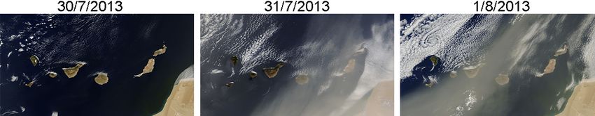
Figure 1. H2 O (left panel) and δD profiles (right panel) as measured by ISOWAT above the subtropical Atlantic close to Tenerife between
10:00 and 13:00 UT on 6 days at the end of July 2013. The depicted data are 10 m vertical averages. For comparison we also depict the
a priori profiles used for the MUSICA NDACC/FTIR and METOP/IASI remote sensing retrievals (grey dashed lines).
dry air was then humidified in a small temperature-stabilized laser frequencies between 7183.5 and 7184 cm−1 . For more
bubbler system. Calibrations were performed 2–5 times per details see the Picarro website (http://www.picarro.com).
flight at varying altitudes in order to check the performance In March 2012 we installed a Picarro L2120-i water iso-
of ISOWAT under all environmental conditions. By combin- topologue analyser at the Izaña Observatory at 2370 m a.s.l.
ing the ground-based and in-flight calibration measurements The measured H2 O and δD time series is depicted in the left
we were able to provide a robust accuracy estimate for the graphs of Fig. 2. In June 2013 we installed an additional Pi-
ISOWAT in-flight data. For the majority of conditions en- carro L2120-i analyser at a small observatory located close
countered, ISOWAT provided profile measurements with an to the cable car summit station of the Teide mountain (at
accuracy for δD of about 10 ‰. Below 2000 ppmv the ac- 3550 m a.s.l.). The Teide H2 O and δD time series is depicted
curacy increases and can exceed 35 ‰ for a humidity below in the right graphs of Fig. 2. We only depict data measured
500 ppmv. during the second half of each night (between midnight and
The ISOWAT humidity data are calibrated against a com- 1 hour after sunrise). By this measure we avoid that the mea-
mercial hygrometer (Edge Tech model Dew Master). We es- surements are affected by local upslope flow, which can bring
timate a precision and accuracy of about 4 %. boundary layer air to the mountain observatories. The mea-
ISOWAT measures the isotopologues with a temporal res- surement gaps are due to instrumental problems when the in-
olution of 1 s. This translates to a horizontal spatial resolution struments were sent to the manufacturer for repair. The time
of about 80 m depending on the aircraft velocity. During the series document that the atmospheric water vapour fields are
MUSICA campaign, profile flights consisted in a relatively rather variable already on hourly timescales.
fast ascent followed by a slower descent with intermediate The δD calibration procedure for the Picarro instruments
level flights at certain selected altitudes and we achieved an is based on a standard delivery module (SDM). It consists of
average vertical resolution of about 1.2 m. The good tempo- two syringe pumps and allows injecting two different stan-
ral resolution of ISOWAT allows observing the rather sharp dards into the vaporizer where a constant dry air flow sus-
vertical gradients encountered during the flights (see Fig. 1). tains immediate evaporation of the liquid in the air stream
For a more detailed report about the aircraft campaign, (for more details see also Aemisegger et al., 2012). The cali-
the ISOWAT measurements, and the calibration procedures bration is made every 8 h. It uses two different δD standards
please refer to Dyroff et al. (2015). (at −142.2 and −245.3 ‰) that are analysed by the instru-
ment at three different humidity levels covering the typical
2.2 Surface-based Picarro humidity range at Izaña and at Teide (during summer).
The precision of our 0.6 Hz measurements was 13.5 and
2 ‰ at 500 and 4500 ppmv, respectively. This noise almost
Similar to ISOWAT, the Picarro water isotopologue analy-
completely averages out in the 10 min averages (our final
sers work with a tunable diode laser. The laser light enters
data product). The random uncertainty of the individual cali-
a cavity filled with the air mass to be analysed. The absorp-
brations (performed every 8 h) was 0.5 and 0.2 ‰ at 500 and
tion signal of the air mass is determined by the ring-down
4500 ppmv, respectively, which also averages out on longer
time of the laser light intensity. In order to get an absorp-
timescales. Systematic uncertainties of the used standard
tion spectrum the ring-down time is measured for different
www.atmos-meas-tech.net/8/483/2015/ Atmos. Meas. Tech., 8, 483–503, 2015486 M. Schneider et al.: Empirical validation of δD remote sensing products
Figure 2. H2 O (upper panel) and δD data (bottom panel) as measured by the Picarro instruments on Tenerife between midnight and 1 hour
after sunrise. The depicted data are 10 min averages obtained during a large amount of different days (numbers as given in the panel). For
comparison we also depict the a priori values used for the MUSICA NDACC/FTIR and METOP/IASI remote sensing retrievals (grey dashed
lines).
water and uncorrected humidity dependence were 1.7 and ratory (a shipping container equipped with electricity, air-
0.7 ‰ at 500 and 4500 ppmv, respectively. conditioning, internet, etc.) and just about 50 m away from
Our Picarro humidity data are calibrated with respect to the Observatory’s main building. Typically we measure on
humidity data measured by standard meteorological sensors. about 2–3 days per week. The number of measurement days
The humidity values measured by the Picarro and the me- is mainly limited by manpower, which is needed for oper-
teorological sensors are very strongly correlated and for the ating the instrument. Ground-based FTIR systems measure
calibrated data we estimate a precision and accuracy of better high-resolution mid-infrared solar absorption spectra. The
than 2 %. spectra contain absorption signatures of many different atmo-
A more detailed description of the MUSICA Picarro in situ spheric trace gases. Therefore, the technique can simultane-
measurements at Tenerife island is the subject of a dedicated ously monitor many different atmospheric trace gases. Con-
paper, which is currently in preparation. tinuous developments of sophisticated retrieval algorithms
allow also the retrieval of tropospheric water vapour isotopo-
logues (for retrieval details please refer to Schneider et al.,
3 The investigated remote sensing products 2006b, 2010b).
Using the measured spectra for estimating the atmospheric
The characteristics of the water vapour isotopologue remote trace gas distributions is generally an ill-posed problem. For
sensing products are rather complex. Schneider et al. (2012) this purpose the solution state is constraint towards an a priori
introduce a proxy state concept that allows for reasonably state. The H2 O and δD a priori values applied for the isotopo-
characterizing the interesting products, namely humidity (or logue retrievals are depicted in Fig. 1 as grey line. The MU-
H2 O) and δD (or HDO/H2 O). They identify two product SICA FTIR retrieval works with several spectral microwin-
types. Product type 1 is a vertical H2 O profile and product dows between 2655 and 3025 cm−1 and with HITRAN 2008
type 2 is for isotopologue studies. Product type 2 provides (Rothman et al., 2009) spectroscopic parameters, and the
H2 O and δD data that are representative for the same air mass H2 O and HDO parameters have been adjusted for speed-
and assures that the δD product is optimally independent on dependent Voigt line shapes (Schneider et al., 2011), which
H2 O. In the following we use this proxy state concept for affects pressure broadening parameters but also line intensi-
briefly discussing the characteristics of the MUSICA remote ties. For H2 O the adjustment has been made taking coinci-
sensing products that are available for the area of Tenerife dent H2 O profile observations as the reference. For HDO the
island. adjustment is more uncertain, since the atmospheric HDO
state was calculated from the measured H2 O state assum-
3.1 Ground-based NDACC/FTIR ing standard δD profiles (there were no HDO measurements
available).
Ground-based FTIR remote sensing measurements have
The averaging kernel is an important output of the re-
been performed at Izaña since 1999 (e.g. García et al., 2012).
trieval. It describes the response of the retrieval on actual
The experiment is situated in its own measurement labo-
Atmos. Meas. Tech., 8, 483–503, 2015 www.atmos-meas-tech.net/8/483/2015/M. Schneider et al.: Empirical validation of δD remote sensing products 487
NDACC / FTIR (type 1) NDACC / FTIR (type 2)
15 15 15 15
2.4 km 2.4 km
4.9 km 4.9 km
7.2 km 7.2 km
9.8 km 9.8 km
10 10 10 10
altitude [km]
altitude [km]
5 5 5 5
DOFS: 2.95 DOFS: 1.73
0 0 0 0
-0.2 0.0 0.2 0.4 0.6 -0.2 0.0 0.2 0.4 0.6 -0.2 0.0 0.2 0.4 0.6 -0.2 0.0 0.2 0.4 0.6
15 15 15 15
10 10 10 10
altitude [km]
altitude [km]
5 5 5 5
DOFS: 1.74 DOFS: 1.71
0 0 0 0
-0.2 0.0 0.2 0.4 0.6 -0.2 0.0 0.2 0.4 0.6 -0.2 0.0 0.2 0.4 0.6 -0.2 0.0 0.2 0.4 0.6
Figure 3. Typical row kernels for the {H2 O, δD}-proxy states as retrieved from Izaña’s ground-based NDACC/FTIR spectra. Left panel of
graphs: product type 1 kernels; Right panel of graphs: product type 2 kernels. The upper graphs of each panel display how the retrieved H2 O
is affected by actual H2 O variations (left graph) and by actual δD variations (right graph). The lower graphs of each panel display the same
for the retrieved δD. For more details on the proxy state kernels see Schneider et al. (2012).
atmospheric variability. The left panel of graphs in Fig. 3 dependency of the retrieved δD on humidity, i.e. the cross-
shows typical averaging kernels for the product type 1 {H2 O, dependency on humidity (compare the bottom left graphs be-
δD}-state. The panel consists of four graphs. The upper left tween the type 1 and type 2 panels).
graph demonstrates how actual atmospheric H2 O affects re- The Izaña FTIR product type 2 offers a degree of free-
trieved H2 O, the upper right graph how actual atmospheric dom for the signal (DOFS, trace of the averaging kernel ma-
δD affects retrieved H2 O, the bottom right graph how ac- trix quantifying the retrieval’s independency on the a priori
tual atmospheric H2 O affects retrieved δD, and the bottom assumptions) for H2 O and δD of typically 1.75. The lower
left graph how actual atmospheric δD affects retrieved δD. tropospheric kernels have an FWHM (full width at half max-
Product type 1 offers H2 O profiles (FWHM, full width at imum) of about 2 km and the middle tropospheric kernels
half maximum, of kernels is 2 km in the lower troposphere, a FWHM of about 5–6 km. In Schneider et al. (2012) the
4 km in the middle troposphere, and 6–8 km in the upper tro- lower and middle tropospheric random uncertainty has been
posphere, Schneider et al., 2012), which have been empiri- estimated to be smaller than 2 % for H2 O and 25 ‰ for δD,
cally validated in a variety of previous studies (e.g. Schnei- respectively, whereby measurement noise, spectral baseline
der et al., 2006a; Schneider and Hase, 2009; Schneider et al., uncertainties, and assumed tropospheric a priori temperature
2010a). A further validation of product type 1 is not the sub- are the leading error sources. The systematic uncertainty can
ject of this paper. reach 10 % for H2 O and 150 ‰ for δD. It is dominated by
Product type 2 is for isotopologue studies and shall be in- uncertainties in the spectroscopic parameters (intensity and
vestigated in this paper. The type 2 product is calculated with pressure broadening). The a posteriori correction method re-
the a posteriori correction method as presented in Schneider duces the δD cross-dependency on humidity to less than 10–
et al. (2012). The respective {H2 O, δD}-state averaging ker- 15 ‰.
nels are depicted as the graphs in the right panel of Fig. 3.
The a posteriori correction significantly reduces the verti- 3.2 Space-based METOP/IASI
cal resolution of the retrieved H2 O state (compare upper left
graphs between type 1 and type 2 panels). This sensitivity IASI is a Fourier transform spectrometer flown aboard the
reduction is mandatory in order to assure that the H2 O prod- METOP satellites. It combines high temporal, horizontal,
uct is representative for the same air mass as the δD product and spectral resolution (covers the whole globe twice a day,
(compare upper left and bottom right graphs in the type 2 measures nadir pixels with a diameter of only 12 km, and
panel). In addition, the a posteriori correction reduces the records thermal radiation between 645 and 2760 cm−1 with a
www.atmos-meas-tech.net/8/483/2015/ Atmos. Meas. Tech., 8, 483–503, 2015488 M. Schneider et al.: Empirical validation of δD remote sensing products
METOP / IASI (type 1) METOP / IASI (type 2)
15 15 15 15
0.0 km 0.0 km
2.3 km 2.3 km
4.9 km 4.9 km
7.2 km 7.2 km
10 10 10 10
altitude [km]
altitude [km]
9.8 km 9.8 km
13.6 km 13.6 km
5 5 5 5
DOFS: DOFS:
3.75 0.67
0 0 0 0
-0.1 0.0 0.1 0.2 0.3 -0.1 0.0 0.1 0.2 0.3 0.00 0.05 0.10 0.00 0.05 0.10
15 15 15 15
10 10 10 10
altitude [km]
altitude [km]
5 5 5 5
DOFS: DOFS:
0.69 0.67
0 0 0 0
-0.1 0.0 0.1 0.2 0.3 -0.1 0.0 0.1 0.2 0.3 0.00 0.05 0.10 0.00 0.05 0.10
Figure 4. As Fig. 3, but for the {H2 O, δD}-proxy states as retrieved from METOP/IASI spectra measured over the subtropical ocean. Please
note the different scales in the x axis for the type 1 and type 2 kernels. For more details on the METOP/IASI proxy state kernels see Schneider
et al. (2012) and Wiegele et al. (2014).
resolution of 0.5 cm−1 ). IASI measurements are assured until logical radiosondes, ground-based FTIR, and the EUMET-
2020 on three different METOP satellites, whereby the first SAT METOP/IASI product and in Wiegele et al. (2014) by
two are already in orbit: MetOp-A has been launched in Oc- comparison to ground-based FTIR at three different locations
tober 2006, MetOp-B in September 2012. For our study we (polar, mid-latitudinal and subtropical) and a further valida-
consider spectra measured by the IASI instruments aboard tion of this type 1 product is not the subject of this paper.
both satellites. Each IASI instrument has two Tenerife over- Interesting for isotopologue studies is product type 2
passes a day (about 10:30 and 22:30 UT). For MUSICA which shall be further investigated in this paper. The respec-
we work so far only with overpasses that observe clear sky tive {H2 O, δD}-state kernels are depicted in the right panel
scenes. We use very strict cloud-screening conditions and of graphs in Fig. 4. The sensitivity is typically limited to
therefore work with only about 10 % of all possible overpass between 2 and 8 km altitude, with a maximum in the mid-
spectra. dle troposphere around 4–5 km. The random uncertainty for
The retrieval uses the spectral window between 1190 and type 2 H2 O and δD is estimated to be about 5 % and 20 ‰,
1400 cm−1 and HITRAN 2008 (Rothman et al., 2009) spec- respectively, whereby measurement noise, surface emissiv-
troscopic line parameters. The applied a priori values are the ity, assumed tropospheric a priori temperature, and unrecog-
same as for the FTIR retrievals and are depicted in Fig. 1 nized thin elevated clouds are the leading error sources. The
as grey line. Schneider and Hase (2011) present our IASI re- systematic uncertainty is very likely dominated by errors in
trieval algorithm as well as a first theoretical error assessment the spectroscopic line parameters and can reach 2–5 % for
of the respective H2 O and δD products. H2 O in the case of a 2–5 % error in the line intensity param-
The left panel of graphs in Fig. 4 shows typical averag- eter. For δD the systematic uncertainty can reach 50 ‰ in
ing kernels for the product type 1 {H2 O, δD}-state of MU- the case of inconsistencies of 5 % between the spectroscopic
SICA IASI retrievals corresponding to spectra measured over intensity parameters of H2 O and HDO. Despite the a pos-
the subtropical northern Atlantic. Product type 1 offers ver- teriori correction there remains a δD cross-dependency on
tical H2 O profiles with the FWHM of the kernels of about humidity, which can cause an additional δD uncertainty of
2 km in the lower and middle troposphere and 3 km in the 30–50 ‰ (Wiegele et al., 2014).
upper troposphere (see upper left graph in type 1 panel of
Fig. 4 and Schneider and Hase, 2011; Wiegele et al., 2014,
for more a more detailed characterization). The MUSICA
product type 1 IASI H2 O profiles are empirically validated
in Schneider and Hase (2011) by comparison to meteoro-
Atmos. Meas. Tech., 8, 483–503, 2015 www.atmos-meas-tech.net/8/483/2015/M. Schneider et al.: Empirical validation of δD remote sensing products 489
4 Assessing random uncertainty and bias 29
Remote sensing data do not represent a single altitude. In-
stead they reflect the atmospheric situation as averaged out
over a range of different altitudes (the kind of averaging is
documented by the averaging kernels of Figs. 3 and 4). Such
latitude [°]
data can only be quantitatively compared to reference data 28
that are available as vertical profiles. Here we compare the
NDACC/FTIR and METOP/IASI products (product type 2,
see Schneider et al., 2012) to the in situ profiles as measured
by ISOWAT between 200 and 6800 m a.s.l.
For a quantitative comparison we have to adjust the ver-
tically highly resolved ISOWAT profiles (xIW as depicted in 27
Fig. 1) to the modest vertical resolution of the remote sens-
ing profiles. For this purpose we first perform a smoothing
-17 -16 -15
towards the altitude grid of the remote sensing retrieval’s for-
longitude [°]
ward model. It can be described by MxIW , whereby M is a
v × w matrix with v and w being the numbers of the grid Figure 5. Site map indicating the location of the different instru-
points of the forward model and of the vertically highly re- ments and ground pixels during the aircraft campaign on 6 days in
solved ISOWAT profile, respectively. This smoothing works July 2013. Green star: Izaña observatory (location of the first Pi-
in a way that assures a conservation of the partial columns carro and the FTIR); blue star: Teide observatory (location of the
between two forward model grid points (i.e. the respective second Picarro); grey lines: aircraft flight track during ISOWAT
partial columns are very similar, before and after the smooth- measurements; black squares and diamonds: cloud-free ground pix-
ing process). In a second step we convolve M xIW with the els of IASI-A and -B, respectively, during the six aircraft flights;
remote sensing averaging kernel Â: coloured filled squares and diamonds: pixels that fulfil our coinci-
dence criteria for IASI-A and -B, respectively (the colours mark the
x̂IW = Â (MxIW − xa ) + xa . (2) different days in analogy to Fig. 1).
Here xa is the a priori profile used by the remote sensing
retrieval. When using the {H2 O, δD}-proxy state averaging
kernels as depicted in Figs. 3 and 4 we have to make sure ISOWAT profile measurement, takes about 3 hours and is
that M xIW in Eq. (2) is in the {H2 O, δD}-proxy state. The re- made over the ocean (see flight tracks of Fig. 5). This is in
sult of this convolution is an ISOWAT profile (x̂IW ) with the contrast to the FTIR remote sensing measurements, which
same vertical resolution as the remote sensing profile. In the need only about 10 min and are made at Izaña observatory
following we will use the “hat”-index for marking parame- at 2370 m a.s.l. on a mountain ridge of an island. It is well
ters or amounts that are retrieved from measured spectra or documented (e.g. Rodríguez et al., 2009) that the immedi-
obtained by convolution calculations according to Eq. (2). ate surroundings of the island at this altitude are affected by
The ISOWAT profiles are limited to 200–6800 m altitude, mixing from the marine boundary layer (MBL). This mixing
whereas the FTIR and IASI remote sensing instruments are is mostly thermally driven: it is weak during the night and
also sensitive to altitudes above 7000 m (and IASI is also starts increasing during the morning hours and the air mass
very weakly sensitive for altitudes below 200 m). For the measured at or very close to the island becomes more and
comparison study we extend the ISOWAT profiles above the more affected by the MBL. At the end of the morning this air
aircraft’s ceiling altitude by the values we use as a priori for mass is not well representative for the situation encountered
the remote sensing retrievals (the a priori values are the same at the same altitude over the ocean.
for FTIR and IASI and depicted as grey dashed line in Fig. 1). For this study we compare the ISOWAT profile with the
Below 200 m altitude we use the values as measured during FTIR data obtained from the spectra measured in the morn-
the first 100 m of available aircraft data. ing with a solar elevation angle of 30◦ . This elevation as-
sures that the FTIR has good sensitivity (absorption pathes
4.1 NDACC/FTIR are short enough and water vapour lines are not too heavily
saturated) and it occurs only about 2:30 h after sunrise, when
When comparing two atmospheric measurements we have to the influence of the MBL on the immediate surroundings of
take care that the different instruments detect the same (or at the island is still moderate.
least very similar) air masses. Large differences in the verti- In Fig. 6 we compare the H2 O measurements. The data
cal resolution can be accounted for by Eq. (2). In addition we are depicted as difference to the a priori, i.e. we discuss here
have to be aware that ISOWAT measures the profile aboard the variability that is actually introduced by the remote sens-
a descending and ascending aircraft. Each flight, i.e. each ing measurement and observed by ISOWAT. Here and in the
www.atmos-meas-tech.net/8/483/2015/ Atmos. Meas. Tech., 8, 483–503, 2015490 M. Schneider et al.: Empirical validation of δD remote sensing products
ISOWAT (FTIR grid) ISOWAT (FTIR resolution) FTIR
7
6
21
altitude [km]
22
5
24
25
4
30
31
3 ^
Mx - x x - x
IW a IW a
2
-100 0 100 -100 0 100 -100 0 100
H O difference to apriori [%]
2
Figure 6. Comparison of ISOWAT and FTIR H2 O measurements (one coincidence for each of the days 21, 22, 24, 25, 30, and 31 of
July 2013). Shown are differences with respect to the a priori profiles. Left panel: ISOWAT data represented for the FTIR altitude grid;
central panel: ISOWAT data convolved with the FTIR kernels, i.e. representative for the vertical resolution of the FTIR; right panel: FTIR
data measured at the end of the morning when solar elevation is still < 30◦ . Depicted are also lower and middle tropospheric error bars for
day 130730 (dry conditions) and 130731 (humid conditions), which are hardly discernible, since the H2 O errors are only a few percent.
following we calculate the H2 O differences as differences Furthermore, we calculate the typical/mean scatter as pre-
between the logarithms of the H2 O concentrations. Since dicted from the combined uncertainties of the remote sensing
1 ln X ≈ 1X X we can interpret these differences between the and the convolved ISOWAT data, ˆRS and ˆIW , respectively:
logarithms of the H2 O concentrations as relative differences. n q
The graphs also show the predicted uncertainties for the 1X
ˆDIFF = ˆ 2 + ˆIW,i
2 . (5)
lower and middle troposphere and for dry (day 130730) and n i=1 RS,i
humid conditions (day 130731). The respective error bars are
hardly discernible, since the H2 O errors are only a few per- For comparison we also calculate a parameter, which is the
cent. Please note that the uncertainties as shown in the cen- scatter in the convolved ISOWAT data:
tral graph take into account the assumption of climatologic v
u n
u1 X 2
a priori values for altitudes above the aircraft’s ceiling alti- σ̂IW = t x̂IW,i − µ̂IW (6)
tude (no measurements!), which is the reason for the relative n i=1
large uncertainty as estimated for the middle troposphere for
the ISOWAT data smoothed by the FTIR kernels. n
whereby µ̂IW = n1
P
x̂IW,i . The σ̂IW parameter informs
The comparison between the left and the central panels of i=1
Fig. 6 gives insight into the vertical structures that can be about the random uncertainty of the water vapour state when
resolved by the remote sensing measurements. The profiles no measurements are available (a priori uncertainty).
depicted in the central and the right panels represent the same The values that result from these calculations for the
vertical structures and their comparison allows conclusions comparison of FTIR and ISOWAT H2 O data are depicted
about the quality of the remote sensing data. in Fig. 7. In the left graph, the scatter between FTIR and
For this purpose we statistically analyse the differences be- ISOWAT (parameter σ̂DIFF according to Eq. 4) is shown as
tween the remote sensing product (x̂RS ) and the convolved black triangles, together with the predicted scatter (ˆDIFF ac-
ISOWAT product (x̂IW , see Eq. 2). We determine the mean cording to Eq. (5), red dashed line). We observe a scatter of
difference b̂DIFF from the n numbers of coincidences: about 28 and 20 % for the lower and middle troposphere, re-
n
spectively. In the lower troposphere the observed scatter is
1X significantly larger than the scatter predicted from the com-
b̂DIFF = x̂RS,i − x̂IW,i (3)
n i=1 bined uncertainties, which might be caused by the fact that
the two instruments observe similar, but not the same air
and the standard deviation of the differences (the scatter be- masses. The large inhomogeneity in the tropospheric water
tween both data sets): vapour fields becomes clearly visible in Fig. 1 (spatial in-
v homogeneity) and Fig. 2 (temporal inhomogeneity). In this
u n
u1 X 2 context the observed scatter has to be interpreted as a rather
σ̂DIFF = t x̂RS,i − x̂IW,i − b̂DIFF . (4) conservative empirical estimation of the FTIR’s random un-
n i=1
certainty. The blue solid line depicts the scatter between the
six ISOWAT profiles when smoothed with the FTIR kernels
Atmos. Meas. Tech., 8, 483–503, 2015 www.atmos-meas-tech.net/8/483/2015/M. Schneider et al.: Empirical validation of δD remote sensing products 491
Assessment of random uncertainty Assessment of bias
7 7
^
^ b
DIFF
DIFF
^
^ +/- [ /sqrt(n-1)]
6 DIFF 6 DIFF
^
/sqrt(n-1)
DIFF
altitude [km]
5 5
for com-
parison:
^
4 IW
4
IW
3 3
2 2
0 25 50 -50 0 50
H O scatter [%] H O mean difference [%]
2 2
Figure 7. Left graph, assessment of the random uncertainty. Black symbols: the FTIR-ISOWAT scatter (σ̂DIFF value according to Eq. 4).
Red dashed line: the predicted scatter (ˆDIFF value according to Eq. 5). Blue solid line: the scatter in the convolved ISOWAT data (σ̂IW value
according to Eq. 6). Blue dashed line: the uncertainty in the not convolved ISOWAT data (IW ). Right graph, assessment
√ of the bias. Black
symbols and error bars: the FTIR-ISOWAT mean difference and standard error of the mean (b̂√DIFF and σ̂DIFF / n − 1 values according to
Eqs. (3) and (4), respectively). Red area: the predicted uncertainty range (calculated as ˆDIFF / n − 1).
ISOWAT (FTIR grid) ISOWAT (FTIR resolution) FTIR
7
6 21
22
altitude [km]
5
24
25
30
4
31
3 ^
Mx - x x - x
IW a IW a
2
-100 0 100 -100 0 100 -100 0 100
D difference to apriori [%]
Figure 8. As Fig. 6, but for δD. Here the error bars are clearly discernible.
(the σ̂IW values according to Eq. 6). It is much larger than to the combined random uncertainties√ of ISOWAT and FTIR
the scatter in the difference with the FTIR profiles meaning (this area is calculated as ˆDIFF / n − 1, see Eq. 5). The ob-
that the FTIR well follows the ISOWAT reference, which served differences overlap well with this area meaning that
confirms previous empirical validation exercises made for we cannot observe a significant bias between the FTIR and
H2 O (e.g. Schneider et al., 2006a; Schneider and Hase, 2009; the ISOWAT data.
Schneider et al., 2010a). Please note that the depicted red The coincident δD profiles are shown in Fig. 8. Here the
dashed line represents the combined uncertainty of the con- predicted uncertainties are clearly discernible. The results of
volved ISOWAT data and the FTIR data. The pure ISOWAT the statistical analysis of the δD comparison are presented
uncertainty (uncertainty of ISOWAT if not convolved with in Fig. 9. In the left graph we observe a scatter (σ̂DIFF ) of
the FTIR kernel, IW ) is much smaller and depicted as blue about 45 and 15 ‰ for the lower and middle troposphere,
dashed line. respectively, which can be interpreted as a conservative em-
The mean difference between FTIR and ISOWAT and pirical estimation of the FTIR’s random uncertainty. In the
the respective
√ standard error of the mean (b̂DIFF and middle troposphere this observed scatter is clearly smaller
σ̂DIFF / n − 1, according to Eqs. (3) and (4), respectively) than the predicted one (ˆDIFF ) indicating that our theoretical
are shown in the right graph of Fig. 7 as black triangles and ISOWAT and/or FTIR error estimations might be too conser-
error bars. The red area depicted around the zero line indi- vative. In particular the ISOWAT estimates are rather con-
cates the zone where a bias might be observed accidently due servative since we assumed that on a single day all δD errors
www.atmos-meas-tech.net/8/483/2015/ Atmos. Meas. Tech., 8, 483–503, 2015492 M. Schneider et al.: Empirical validation of δD remote sensing products
Assessment of random uncertainty Assessment of bias
7 7
^
^
b
DIFF DIFF
^ ^
+/- [ /sqrt(n-1)]
6 DIFF 6 DIFF
^
/sqrt(n-1)
DIFF
for com-
altitude [km]
5 5
parison:
^
IW
4 IW
4
3 3
2 2
0 25 50 75 -50 0 50
0 0
D scatter [ / ] D mean difference [ / ]
00 00
Figure 9. As Fig. 7, but for δD.
H O D
2 -100
FTIR H O [ppmv]
3000
]
00
D [ /
0
-200
2
2000 21
FTIR
22
24
-300
25
1000
30
31
1000 2000 3000 -300 -200 -100
^ ^ 0
ISOWAT H O (x ) [ppmv] ISOWAT D (x ) [ / ]
2 IW IW 00
Figure 10. Correlation between ISOWAT data (smoothed with FTIR kernels) and FTIR data for 5 km altitude (left for H2 O and right for
δD). Black line is the 1 : 1 diagonal and red dotted line is the 1:1 diagonal shifted by +60 ‰. Error bars represent the ISOWAT and FTIR
uncertainty estimations. Note that a large part of the uncertainty in the smoothed ISOWAT data is due to the fact that there are no ISOWAT
measurements above the aircraft’s ceiling altitude.
that occur at different altitudes and during ascent and descent to detect a significant bias. It is about 25 ‰ in the lower tro-
are fully correlated. Allowing for δD errors that are not fully posphere and 70 ‰ in the middle troposphere.
correlated (for instance positive errors at 2 km altitude and In Fig. 10 we show a correlation plot for the H2 O and
negative errors at 5 km altitude) would strongly decrease the δD data as observed in the middle troposphere (altitude of
error as estimated for the ISOWAT data, since through the 5 km) by ISOWAT and FTIR. This plot can serve as a sum-
convolution with the kernel a large part of the error would mary of the comparison exercise: (1) H2 O and δD signals are
cancel out. The comparison of the observed scatter with the similarly observed by both instruments (good correlation),
blue solid line (scatter between the six convolved ISOWAT (2) there is no significant difference between the H2 O data,
profiles, σ̂IW ) demonstrates that the FTIR δD product well and (3) there is a significant positive bias in the FTIR δD
captures the atmospheric variations as seen by the ISOWAT data.
reference data.
The right graph of Fig. 9 reveals a clear systematic differ- 4.2 METOP/IASI
ence between the FTIR and the ISOWAT δD data.
At and above 3 km altitude this difference lies outside the
The black squares and diamonds in Fig. 5 show all the IASI-
zone where a bias might be observed accidentally due to the
A and IASI-B pixels for morning overpasses that have been
combined random uncertainties of ISOWAT and FTIR (red
declared cloud free (according to EUMETSAT level 2 data)
area calculated according to Eq. 5), meaning that we are able
within a 250 km × 250 km area around the aircraft’s flight
tracks. In order to assure that IASI and ISOWAT observe
Atmos. Meas. Tech., 8, 483–503, 2015 www.atmos-meas-tech.net/8/483/2015/M. Schneider et al.: Empirical validation of δD remote sensing products 493
H O D
2 -100
3000
IASI H O [ppmv]
]
00
D [ /
0
-200
2
IASI
2000
24
-300
25
1000 30
31
1000 2000 3000 -300 -200 -100
^ ^ 0
ISOWAT H O (x ) [ppmv] ISOWAT D (x ) [ / ]
2 IW IW 00
Figure 11. As Fig. 10, but for correlation between ISOWAT data (here smoothed with IASI kernels, i.e. this ISOWAT data are different to
the ISOWAT data as depicted in Fig. 10) and IASI data for 5 km altitude. Three H2 O outliers on day 130731 (blue triangles) are marked by
black edges. For clarity the error bars are only given for one observation per day and on day 130731 in addition for one of the three outliers.
similar air masses we only work with IASI observations that Table 1. Scatter values as obtained from IASI and ISOWAT coinci-
are made not further away than 50 km from the typical lo- dences that fulfil our coincidence criteria (presents the same as the
cation of the aircraft. This yields 13 coincidences (three for left panels of Figs. 7 and 9, but for IASI instead of FTIR and at 5 km
IASI-A and ten for IASI-B) made on four different days: altitude only). Predicted: combined ISOWAT and IASI estimated
130724, 130725, 130730, and 130731. The respective pix- uncertainties (ˆDIFF ); IASI − ISOWAT: scatter as observed in the
difference between ISOWAT and IASI (σ̂DIFF ); ISOWAT: scatter as
els are marked by the filled squares and diamonds in Fig. 5
observed in the ISOWAT data (σ̂IW ). The values in parenthesis are
(the different colours are for the different days). for calculations without considering the three outliers on 130731.
IASI can hardly measure the vertical distribution of δD
(see right panel of Fig. 4). For this reason we can limit the H2 O [%] δD [‰]
validation exercise to a single altitude level where IASI has
typically good sensitivity. This is the case for the altitude Predicted (ˆDIFF ) 9.9 (8.5) 13.2 (12.3)
of 5 km, which typically represents the atmospheric situation IASI − ISOWAT (σ̂DIFF ) 16.0 (6.0) 12.0 (13.2)
between 2 and 8 km altitude. ISOWAT (σ̂IW ) 29.9 (34.4) 37.1 (36.7)
Figure 11 shows the same as Fig. 10 but for the IASI in-
stead of the FTIR data. It depicts the correlation between the
ISOWAT data (convolved with IASI kernels) and the IASI this quantitatively, we compare the scatter observed in the
data. difference between IASI and ISOWAT with the scatter ob-
For H2 O the data group nicely around the 1 : 1 diagonal. served in the ISOWAT profiles as well as with the scatter pre-
For three of the five IASI observations on day 130731 the dicted from our ISOWAT and IASI uncertainty estimations.
agreement is unusually poor. These data points are marked These scatter values are collected in Table 1. First, we see
by black edges and they correspond to the one IASI-A pixel that the scatter in the IASI − ISOWAT difference (the value
and the two IASI-B pixels marked by the black edges in σ̂DIFF according to Eq. 4) is much smaller than the scatter
Fig. 5. The reason for their relatively poor agreement is that in the convolved ISOWAT data (the value σ̂IW according to
for these coincidences the two IASI and ISOWAT instru- Eq. 6), i.e. IASI well tracks the H2 O and δD variations as
ments observe different air masses. For more details see Ap- observed by ISOWAT. From the σ̂DIFF values we empirically
pendix A. For δD we observe a good correlation but there is assess an IASI random uncertainty of better than 6–16 % for
a significant systematic difference. All the IASI data show H2 O and about 13 ‰ for δD. For the latter the value is not
rather consistently about 60 ‰ less HDO depletion than larger than the combined estimated errors of the convolved
ISOWAT and this bias is outside the predicted uncertainty ISOWAT and the IASI δD data (ˆDIFF according to Eq. 5),
range, i.e. it is significant. In this context it is interesting that which is also about 13 ‰. Since ISOWAT and IASI actu-
for the FTIR data we observe a similar systematic difference, ally do not detect the same air mass, part of the observed
which confirms the work of Schneider and Hase (2011) and scatter should be due to the observation of a different air
Wiegele et al. (2014), where no systematic differences be- mass. Consequently our combined uncertainty estimations
tween IASI and FTIR are reported. are very likely too conservative, which might be explained
The good correlations as seen in Fig. 11 demonstrate that by the aforementioned conservative ISOWAT uncertainty as-
IASI can well capture the variations of the middle tropo- sumption (assumption of fully correlated errors).
spheric water vapour isotopologues. In order to document
www.atmos-meas-tech.net/8/483/2015/ Atmos. Meas. Tech., 8, 483–503, 2015494 M. Schneider et al.: Empirical validation of δD remote sensing products
4.3 Bias in the remote sensing data 0
When comparing the remote sensing and ISOWAT H2O data
we find a systematic difference of up to 10 %. However, the -200
]
00
mean difference is clearly smaller than the respective stan-
D [ /
0
dard error of the mean, making this empirical bias estimation
statistically insignificant (see black triangles and error bars -400
ISOWAT (nearby TFE)
in the right panel of Fig. 7). Since the lower/middle tropo- Picarro (at TFE)
spheric H2 O fields are temporally and spatially very variable Picarro (at KA)
Rayleigh
(variability in the range of 50–150 %), it is difficult to iden- -600
Mixing
tify a bias in the H2 O remote sensing product using a limited
1000 10000
number of nearby in situ reference observations. H O [ppmv]
2
Tropospheric δD variability is in the range of 50–
150 ‰ and a remote sensing δD bias of a similar magni- Figure 12. δD–H2 O plot using in situ observations made from
tude might be detected even by using a small number of different platforms (aircraft/ISOWAT and surface/Picarro) and at
coinciding reference measurements. In fact the bias we ob- different sites (mid-latitudes at Karlsruhe, KA, and subtropics at
serve between the few ISOWAT reference data and our re- Tenerife, TFE). Cyan line: Rayleigh curve for initialization with
mote sensing δD product is statistically significant. It is be- T = 25 ◦ C and RH = 80 %. Magenta lines: two mixing lines. First
tween 10 and 70 ‰ for the FTIR (see right panels in Figs. 9 for mixing between H2 O[1] = 25 000 ppmv; δD[1] = −80 ‰ and
and 10) and about 60 ‰ for the IASI data (see right panel of H2 O[2] = 900 ppmv; δD[2] = −430 ‰. Second for mixing between
H2 O[1] = 25 000 ppmv; δD[1] = −80‰ and H2 O[2] = 200 ppmv;
Fig. 11). Wiegele et al. (2014) found consistency between
δD[2] = −610 ‰.
a large amount of IASI and FTIR data obtained at three
rather different locations (subtropics, mid-latitudes and Arc-
tic), which suggests that the biases are similar and stable for a the in situ reference data with the remote sensing averaging
wide range of different locations. However, in order to inves- kernels further increases this risk of misinterpreting the δD
tigate the consistency of the bias for different locations more remote sensing data quality: by convolving the in situ data
quantitatively further ISOWAT profile measurements at dif- with the averaging kernels we create a δD in situ reference
ferent sites and during different seasons would be desirable. that has a similar dependency on H2 O as the remote sensing
data and the good correlation between the remote sensing and
the convolved in situ δD data might partly be a result of the
5 Proofing the added value of δD convolution calculations according to Eq. (2).
For these reasons it is rather important to complement
5.1 The added value of δD observations the quantitative validation exercises as shown in Sect. 4 by
a qualitative study demonstrating that the δD remote sens-
In Fig. 12 we plot all the in situ data that have been measured ing measurements add new information to the H2 O remote
so far in the lower or middle troposphere within the project sensing data. This added value of δD can be examined by
MUSICA. These data represent different altitudes and two analysing δD–H2 O diagrams (we face a two-dimensional
different locations (subtropics and mid-latitudes). We ob- validation problem!). We have to demonstrate that our com-
serve a strong correlation between the logarithm of H2 O con- bined δD/H2 O remote sensing products are really useful for
centrations and δD (for linear correlation we get an R 2 of studying atmospheric moisture transport processes.
about 80 %), which suggests that δD and H2 O contain sim- In this section we work with pure in situ data (not con-
ilar information thereby relativizing the results as presented volved with the remote sensing averaging kernels). This does
in Sect. 4: in Fig. 9 and Table 1 we show that the remote not allow a quantitative study, but it ensures that our in situ
sensing measurements can correctly detect a large part of the reference remains completely independent from the remote
actual δD variations. However, we do not show if the remote sensing data.
sensing δD measurements are precise enough for detecting
the small part of the lower/middle tropospheric δD variations 5.2 Dehydration via condensation versus vertical
that are complementary to H2 O. mixing from the boundary layer
In this context, we have to be aware that the remote sens-
ing retrievals provide δD data that are slightly dependent on The downwelling branch of the Hadley circulation plays a
the atmospheric H2 O state (see the bottom left graphs in the dominating role for the free troposphere (FT) of the sub-
type 1 and 2 panels of Figs. 3 and 4), meaning that the re- tropics. It is responsible for a strong subsidence inversion
mote sensing δD data might be correlated to the in situ δD layer which hinders mixing of planetary boundary layer
data only via its dependency on H2 O and not because δD (PBL) air into the FT. Under such situation the FT air mass
is correctly retrieved. The fact that in Sect. 4 we convolve is transported from higher latitudes and/or higher altitudes
Atmos. Meas. Tech., 8, 483–503, 2015 www.atmos-meas-tech.net/8/483/2015/M. Schneider et al.: Empirical validation of δD remote sensing products 495
(Galewsky et al., 2005; Barnes and Hartmann, 2010; Cuevas PM10 < 2 g / m
3
PM10 > 25 g / m
3
et al., 2013).
In addition, the summertime FT of the northern subtropical 60 60
Atlantic is frequently affected by air masses that are advected
latitude [°]
40 40
from the African continent (e.g. Prospero et al., 2002; Ro-
dríguez et al., 2011; Andrey et al., 2014). At that time of the 20 20
year there are strong and extended heat lows over the African all all
continent at 20–35◦ N. These heat lows modify the transport clean dust
0 0
-80 -60 -40 -20 0 -80 -60 -40 -20 0
pathways to the FT and enable mixing from the PBL to the longitude [°] longitude [°]
FT (e.g. Valero et al., 1992).
These two different transport pathways can be observed Figure 13. 72 h backward trajectories between May and October
at our reference site (island of Tenerife and surroundings), (2012 and 2013) for Izaña classified with respect to the PM10 value
and we can use these circumstances for validating the added as measured in situ at Izaña. Grey lines: all backward trajectories;
value of the δD signal and for demonstrating the usefulness blue lines: for PM10 < 2 µg m−3 ; red lines: for PM10 > 25 µg m−3 .
of the remote sensing data for studying atmospheric moisture
transport processes.
The Izaña Picarro data are paired with Izaña’s PM10
5.2.1 Aerosol data as proxy for transport pathways in situ aerosol measurements. As definition for clean con-
ditions we use PM10 < 2 µg m−3 and for dust conditions
Saharan dust aerosols measured in the FT around Tenerife PM10 > 25 µg m−3 . More information about these data is
can be used for identifying an air mass that has experienced given in Appendix B (Fig. B2). We only work with night-
vertical transport over the African continent. This shall be time data (observed between midnight to 1 hour after sun-
demonstrated by Fig. 13, which shows that at Izaña and rise). Thereby we can minimize the risk of data affected by
in summer high aerosol concentrations (PM10 > 25 µg m−3 ) local mixing between the MBL and the FT.
are clearly correlated to air masses that have been advected At Teide there are no continuous in situ aerosol ob-
from the African continent. The PM10 aerosol data show servations and we pair the Teide Picarro data with the
the aerosol mass concentration considering all particles with Izaña AERONET (http://aeronet.gsfc.nasa.gov) remote sens-
aerodynamic diameter smaller than 10 µm, and at Izaña, ing data. The AERONET photometers analyse the direct
PM10 is, by far, dominated by Saharan dust particles (Ro- sunlight and report the aerosol optical depth (AOD) for the
dríguez et al., 2011). For the calculation of the backward whole atmosphere above Izaña, i.e. they are reasonably rep-
trajectories we use HYSPLIT (Hybrid Single-Particle La- resentative for the altitudes around Teide. For an AOD value
grangian Integrated Trajectory – some examples and expla- at 500 nm below 2 × 10⁻² we assume clean conditions and
nations of the HYSPLIT calculations are given in Cuevas above 5 × 10⁻² dust conditions. In order to avoid that the Pi-
et al., 2013). carro observations are affected by local vertical mixing we
In the following we use low aerosol concentrations as only work with nighttime data (as for the Izaña Picarro we
proxy for an FT air mass that has been mainly transported only use data obtained between midnight and one our after
from higher latitudes and/or higher altitudes (clean condi- sunrise). Note that we have to interpolate to AERONET data
tions, no vertical mixing from the PBL to the FT). High during the nighttime, since the AERONET photometer ob-
aerosol concentrations are our proxy for air masses influ- servations work with direct sunlight.
enced by vertical mixing over the African continent (dust Izaña’s ground-based FTIR remote sensing system has the
conditions). We investigate the isotopologue data measured capability to resolve the first few kilometres above Izaña.
by the different instruments under the different conditions. The Izaña AERONET data are representative for similar air
For each instrument we need aerosol data that are represen- masses and can be used for classifying the FTIR data. We use
tative for a similar air mass as the isotopologue data. the same threshold levels as for the classification of the Teide
For ISOWAT we use the V10 aerosol data observed in situ Picarro data.
during the flights. The V10 aerosol data is the aerosol volume For the classification of the IASI data we also use Izaña’s
concentration considering particles with a diameter smaller AERONET data. However, we have to consider that IASI is
than 10 µm. The vertical resolution of these measurements most sensitive at around 5 km altitude, i.e. an altitude signif-
is 100 m. The ISOWAT data are much higher resolved. We icantly above the location of the Izaña AERONET photome-
calculate 100 m averages from the ISOWAT data in order to ter. In order to have a reasonable proxy for aerosol amounts
make them representative for the same layers as the aerosol around 5 km altitude we work with higher AOD threshold
data. An air mass with V10 < 1 µm3 cm−3 is defined as a values. We use a value below 5 × 10⁻² for clean conditions
clean air mass and an air mass with V10 > 10 µm3 cm−3 is de- and above 1 × 10⁻¹ for dust conditions.
fined as dust air mass. For more details on the aircraft aerosol A brief overview of the Izaña AERONET data is given in
data see Appendix B and Fig. B1. Appendix B (Fig. B3).
www.atmos-meas-tech.net/8/483/2015/ Atmos. Meas. Tech., 8, 483–503, 2015You can also read