Sensitivity of Landsat-8 OLI and TIRS Data to Foliar Properties of Early Stage Bark Beetle (Ips typographus, L.) Infestation - University of ...

Article
Sensitivity of Landsat-8 OLI and TIRS Data to Foliar
Properties of Early Stage Bark Beetle (Ips
typographus, L.) Infestation
Haidi Abdullah 1,*, Roshanak Darvishzadeh 1, Andrew K. Skidmore 1,2 and Marco Heurich 3,4
 1 Faculty of Geo-Information Science and Earth Observation (ITC), University of Twente, P.O. Box 217, 7500
 AE Enschede, The Netherlands; r.darvish@utwente.nl (R.D.); a.k.skidmore@utwente.nl (A.K.S.)
 2 Department of Environmental Science, Macquarie University, NSW 2106, Australia

 3 Department of Conservation and Research, Bavarian Forest National Park, 94481 Grafenau, Germany;

 Marco.Heurich@npv-bw.bayern.de
 4 Chair of Wildlife Ecology and Wildlife Management, University of Freiburg, Tennenbacher Straße 4, D-

 79106 Freiburg, Germany
 * Correspondence: H.j.Abdullah@utwente.nl

 Received: 7 January 2019; Accepted: 13 February 2019; Published: 15 February 2019

 Abstract: In this study, the early stage of European spruce bark beetle (Ips typographus, L.) infestation
 (so-called green attack) is investigated using Landsat-8 optical and thermal data. We conducted an
 extensive field survey in June and the beginning of July 2016, to collect field data measurements
 from several infested and healthy trees in the Bavarian Forest National Park (BFNP), Germany. In
 total, 157 trees were selected, and leaf traits (i.e. stomatal conductance, chlorophyll fluorescence,
 and water content) were measured. Three Landsat-8 images from May, July, and August 2016 were
 studied, representing an early stage, advanced stage, and post-infestation, respectively. Spectral
 vegetation indices (SVIs) sensitive to the measured traits were calculated from the optical domain
 (VIS, NIR, and SWIR), and canopy surface temperature (CST) was calculated from the thermal
 infrared band using the mono-window algorithm. The leaf traits were used to examine the impact
 of bark beetle infestation on the infested trees and to explore the link between these traits and remote
 sensing data (CST and SVIs). The differences between healthy and infested samples regarding
 measured leaf traits were assessed using Student’s t test. The relative importance of the CST and
 SVIs for estimating measured leaf traits was evaluated based on the variable importance in
 projection (VIP) obtained from the partial least squares regression (PLSR) analysis. A temporal
 comparison was then made for SVIs with a VIP > 1, including CST, using statistical significance
 tests. The clustering method using a principal components analysis (PCA) was used to examine
 visually how well the two groups of sample plots (healthy and infested) are separated in 2-D space
 based on principal component scores. Finally, linear regression (LR) was used to generate the leaf
 traits maps using the SVI that have highest VIP score and then used to produce a stress map for the
 study area. The results revealed that all measured leaf traits were significantly different (p < 0.05)
 between healthy versus infested samples. Moreover, the study showed that CST was superior to the
 SVIs in detecting subtle canopy changes due to bark beetle infestation for the three months
 considered in this study. The results showed that CST is an essential variable for estimating
 measured leaf traits with VIP > 1, improving the results of clustering when used with other SVIs.
 Likewise, the stress map produced by CST and leaf traits well presented the infestation areas at the
 green attacked stage. The new insight offered by this study is that the stress induced by the early
 stage of bark beetle infestation is more pronounced by Landsat-8 thermal bands than the SVIs
 calculated from its optical bands. The potential of CST in detecting the green attack stage would
 have positive implications for forest practice.

Remote Sens. 2019, 11, 398; doi:10.3390/rs11040398 www.mdpi.com/journal/remotesensing

Remote Sens. 2019, 11, 398 2 of 23

 Keywords: bark beetle (Ips typographus, L.); green attack; Landsat-8; canopy surface temperature;
 spectral vegetation indices

1. Introduction
 Forests are important ecosystem with economical, social, and ecological values. The economic
value of timber in a forest is typically threatened by natural disturbances such as fire, drought, wind,
snow, and insect or disease outbreaks [1,2]. In Europe, the European spruce bark beetle (Ips
typographus, L.) is a common disturbance agent in forests dominated by Norway spruce (Picea abies)
[3]. Bark beetle infestation extends across ten million hectares of trees in Europe. Much public money
has been invested to compensate forest owners for their economic loss and for the cost of reforestation
[4–6]. In addition to the negative impact on timber production, bark beetles can also have a positive
impact on the ecosystem by providing a suitable habitat in the form of opening forest canopy,
increasing habitat heterogeneity and biodiversity, all of which enhance the survival of other species
[7,8].
 The principle of bark beetles killing host trees has been well described in Wermelinger [9]. After
a successful attack, the trees change colour in three stages; referred to as green, red, and grey attack,
respectively [9,10]. The green attack is the early stage of bark beetle infestation in which the colonised
trees are yet to show distinct symptoms observable by the human eye [11,12]. A red-attack is evidence
of the advanced stage of bark beetle infestation, in which the attacked trees develop stress symptoms
involving turning the colour of their needles from green to yellow to red-brown. Subsequently, the
needles fall from the infested trees, and only the grey bark remains; hence, this stage is termed ‘grey
attack’ [13].
 Detection of bark beetle infestation at the green attack stage means locating infested trees at the
stage where the beetle larvae are still within the tree. Effective measures to manage the beetles can
then be undertaken. This will ultimately help reduce the number of infested trees, lessening the
economic loss. Visual inspections during field surveys and pheromone traps have traditionally been
used to detect bark beetle infestations in Norway’s spruce forests. However, these methods are
subjective, very laborious, costly, and only able to cover relatively small areas. Remote sensing
presents an alternative to existing methods for monitoring and detecting infestations on large spatial
scales [14]. To date, remote sensing data have been successfully used to detect the advanced stages
(red and grey attacks) of bark beetle infestation.
 For example, many studies have employed spectral vegetation indices (SVIs) from low-to-
medium resolution satellite data to detect the advanced stages of bark beetle infestation (red and grey
attack) [12,15–19]; however, to date, the identification of European spruce bark beetle (Ips typographus,
L.) green attack has been less satisfactory due to many biological, technical and logistical
constraints/limitations. These issues include the flight activity of the bark beetle, the time duration
required for the colonisation process and the period when the infested trees have yet to show distinct
symptoms capable of being observed by human eye. Hence, it is important to consider biological as
well as logistical factors when using remotely sensed data to detect bark beetle green attack [20]

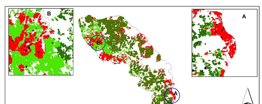
Remote Sens. 2019, 11, 398 3 of 23

 Figure 1. Studies that have used remote sensing data to attempt detecting bark beetle infestation at
 the green attack stage.

 There are very few studies that have paid particular attention to investigating the impact of bark
beetle green attack on biochemical properties and physiological status of infested trees. However,
they studied different beetle (mountain pine beetle) and tree (lodgepole pine) species. For example,
Yamaoka et al. [21] documented a decline in sapwood moisture content resulting from mountain pine
beetle attack. Likewise, Cheng et al. [22] revealed water deficit and changes in chlorophyll content of
artificially stressed pine trees by mountain pine beetle. They also identified the wavelength range
between 950 nm and 1390 nm asa good spectral region able to separate healthy from green attacked
trees. In general, moisture stress in vegetation may result in non-visual symptoms that are detectable
with remote sensing data, particularly in the shortwave and thermal infrared regions, where water
absorption features exist [23–26]. However, the majority of the studies on bark beetle (either
mountain pine beetle or spruce bark beetle) green attack detection with remotely sensed data have
mainly utilised optical remote sensing data (Figure 1). There are few published examples of studies
which investigate the use of temperature, and none which focus on the impact of European spruce
bark beetle infestation on biochemical properties and physiological status of infested trees in the TIR
domain. To our knowledge, only one study, by Hais and Kučera [27], has investigated the impact of
bark beetle (Ips typographus, L.) infestation at the advanced stages (Gray attack) on surface
temperature using thermal infrared (TIR) data. Their study examined the effect of spruce bark beetle
infestation and clear-cutting on surface temperature between 1987 and 2002 in the central part of
Sumava National Park in the Czech Republic. Further, Sprintsin et al. [28] used the surface
temperature calculated from the Landsat 7 ETM+ to detect an early stage of mountain pine beetle
infestation in British Columbia. Although Sprintsin, Chen, and Czurylowicz [28] suggested that
temperature condition indices (TCI) used in their study have the potential to differentiate between
healthy and green attacked pine they could not validate their results due to lack of ground reference
data for their green attacked study areas.
 Numerous studies have shown the significant potential of TIR data to elucidate plant
biophysical and biochemical properties [29–31]. For example, the primary absorption feature that is
associated with leaf water content can be observed in both shortwave and thermal infrared regions
(Table 1) [32,33]. As such, several studies have shown that TIR data have great potential to detect
plant diseases and pathogens before the plants develop visual stress symptoms [34–38]. Moreover,
retrieving the canopy surface temperature (CST) from TIR data is widely used to track vegetation
water status [39]. The surface temperature is interrelated with plant functions, such as
evapotranspiration which is controlled by stomatal conductance [34,40]. Therefore, alterations in
these processes will lead to changes in the air and the surface temperature of leaves [41–44].
Furthermore, physiological studies have shown that the reduction of leaf water content disturbs
stomatal conductance and leads to an increase in leaf surface temperature [45–47]

Remote Sens. 2019, 11, 398 4 of 23

 In addition to water content and stomatal conductance, recent studies have shown that there is
a strong relationship between canopy surface temperature and photosynthetic activity, which can be
measured by chlorophyll fluorescence [36]. Chlorophyll fluorescence has been found to be a reliable
indicator for examining the impact of different stressors (drought, insect infestation, and pathogens)
on plant photosynthesis and the physiological state of vegetation [48,49]. When leaf transpiration rate
decreases (i.e., by closing stomata) both chlorophyll fluorescence and photosynthetic activity will
decrease, while heat dissipation will increase [50]. Hence, chlorophyll fluorescence has been used as
a reliable indicator for monitoring plant water stress [21,51].
 In this study, for the first time, we sought to explore and compare the potential of both optical
and thermal infrared (TIR) data from Landsat-8 for detection of pre-visual symptoms induced by
European spruce bark beetle green attack. We studied the impact of spruce bark beetle green attack
on leaf properties (foliar stomatal conductance, chlorophyll fluorescence, and water content). To do
this, canopy surface temperature (CST) and spectral vegetation indices (SVIs) were calculated using
three Landsat-8 images for May, July, and August 2016, as these months, represent the time of early,
advanced, and after spruce bark beetle green infestation, respectively. Our study benefits from
valuable in situ measurements of leaf traits at the time of infestation that have been used to explain
the impact of bark beetle attacks on Landsat 8 optical and TIR data. Our objectives were as follow: (i)
to assess the potential of CST and SVIs calculated from Landsat 8 data to differentiate between
healthy and infested sample groups; (ii) to study the temporal variation of CST and SVIs under spruce
bark beetle infestation; and (iii) to evaluate the utility of CST and a number of SVIs to estimate
measured leaf traits within infested and healthy samples.

2. Materials and Methods

2.1. Study Site and in Situ Data Collection
 The field campaign was conducted during June and July 2016 in the Bavarian Forest National
Park (BFNP), which is a 24.222 ha forest located in south-eastern Germany along the border with the
Czech Republic, between 13°12’9” E (longitude) and 49°3’19” N (latitude) (Figure 2). The BFNP was
established in 1970, and significantly extended in 1997. Depending on the elevation within the BFNP,
which ranges from 600 m to 1453 m, the mean annual temperature fluctuates between 3.5 °C and 9
°C, and the total annual precipitation varies from 900 mm to 1800 mm [52,53]. The first bark beetle
infestations began in 1984 and, to date, more than 7000 ha have been affected. The strict non-
intervention policy of the National Park offers the possibility of studying bark beetle dynamics
without human interference [52,54].

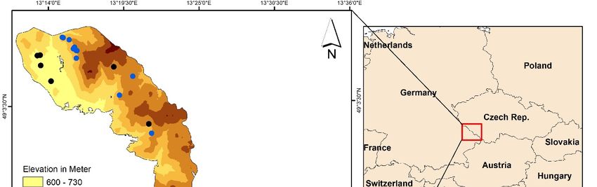
Remote Sens. 2019, 11, 398 5 of 23

 Figure 2. The location of Bavarian Forest National Park in Central Europe.

 We sampled trees from healthy stands and stands with trees freshly infested by the bark beetle.
For the healthy stands, we randomly selected plots (30 m × 30 m) from all over the national park. To
select the green attacked trees, we conducted an extensive field survey to search for dry brown
powder around the trees. Care was taken to only consider those plots with all trees freshly infested
or which were dominated (80%) by freshly green-attack trees. In this way, we were assured that the
extracted remote sensing signature from these plots would not have mixed effects from the attacked
trees of previous years. In total, 40 healthy and 21 infested plots were sampled. The centre of each
plot was measured using Differential Global Positioning System (DGPS) Leica GPS 1200 (Leica
Geosystems AG, Heerbrugg, Switzerland) with an accuracy of better than 1 m after post-processing.
Each of 61 selected plots measured 30 × 30 m to encapsulate the spatial resolution of a Landsat-8 data,
which allows for a 30 m radius buffer zone around the ‘central pixel’ location for uncertainty in spatial
registration of image pixels. By doing this we minimized the potentially confounding influence
(mixed pixels) of green attacked Norway spruce trees.
 From each plot, three to five trees were selected as representative for the plot. Since the height
of Norway spruce trees reaches 25 to 30 m, we used a crossbow to shoot an arrow with a fishing line
attached to a branch with sunlit leaves. The fishing line was used to feed a rope over the targeted
branch from the upper canopy. Once the rope was in place, the branch was pulled down gently until
it broke off. Full details regarding the use of the crossbow can be found in Ali et al. [55]. On average
two to three branches, exposed to sunlight, were taken from the upper part of each tree. Next, needle
samples were taken from the collected branches to measures leaf traits.

2.2. Measurement of Leaf Properties
 In this study, a steady-state instrument SC-1 Leaf Porometer (Decagon Devices Inc. 2365 NE
Hopkins, Court Pullman, WA 99163) was used to measure the needle stomatal conductance. This
instrument computes stomatal conductance using a leaf clip chamber that can monitor the relative
humidity (RH%) released from the leaf stomata. To measure the stomata, a number of needles were
gently attached to cover the chamber port. Since stomata are sensitive to environmental conditions
and physical stress, all the measurements were taken under similar environmental conditions (clear

Remote Sens. 2019, 11, 398 6 of 23

sky, between 11 am to 3 pm local time). An average of three to four measurements was taken for each
sampled tree within each plot (SC-1 Operator’s Manual, 2016).
 Immediately after the stomata measurement, a chlorophyll content meter CCM-330 (Opti-
Sciences, Inc. 8 Winn Ave Hudson, NH 03051 USA) was used to measure the chlorophyll fluorescence
ratio (CFR). This instrument uses the emission ratio of fluorescence at both the red (700 nm) and the
far red (735 nm) part of the electromagnetic spectrum, as proposed by Gitelson et al. [56]. On average
ten readings were taken per sample from each branch. Then, the leaf water content (CW, mg/cm2)
was computed using fresh and dry weight. To do this, three grams of the freshly harvested needles
were weighed from each sample. A portable leaf area meter (AM-350) was used to measure the total
needles’ surface area for each of the three grams considered. Norway spruce needles are cylindrical
and, therefore, this surface area was multiplied by a universal conversion factor of 2.57 [57]. Then, to
acquire the hemispherical-surface projection of the sample surface needles, the total area obtained
was divided by 2. Finally, the needle samples were oven dried for 72 hours at 75 °C, and the dried
weight of each sample was measured. The leaf water content (Cw) was computed using the following
equation [58]:
 Wf − Wd
 w =
 A
where Wf and Wd are the fresh and dry weight, respectively, and A is the sample leaf area.

2.3. Landsat-8 Imagery and Pre-Processing
 Cloud-free Landsat-8 images were obtained from the USGS Global Visualization Viewer
(http://glovis.usgs.gov/) for the months May, July, and August 2016. According to the Bavarian Forest
National Park authorities, the bark beetles of the infestation in 2016 had started to swarm on May 10,
2016. Therefore, the May image was designated as the early stage of bark beetle infestation.
 Landsat-8 has two sensors called OLI and TIRS. The OLI sensor collects data from nine spectral
bands ranging from 0.43–2.29 nm with a 30 m spatial resolution, while the TIRS sensor collects data
from two thermal bands ranging from 10.6–12.5 nm with a 100 m spatial resolution resampled to 30
m in the delivered data product (Table 1).
 For both the OLI and the TIRS sensor, radiance values were calculated, using the coefficient
supplied by USGS. Secondly, for OLI data, a radiometric calibration was applied to convert the
radiance value to top-of-atmosphere (TOA) reflectance. Then, MODTRAN4-based atmospheric
correction software (FLAASH) was used to convert the TOA Reflectance to surface reflectance [59].
Full details regarding the use of FLAASH can be found in [60]. Finally, the reflectance values of the
infested and healthy plots were extracted from the Landsat-8 scenes and were used for further
analysis.

 Table 1. The Landsat-8 sensors, the operational land imager (OLI), and the thermal infrared sensor
 (TIRS) spectral bands and their spatial resolution.

 Resoultion
 Bands Wavelength (micrometers)
 (meters)
 Band-1 (Coastal aerosol) 0.43–0.45 30
 Band-2 (Blue) 0.45–0.51 30
 Band-3 (Green) 0.53–0.59 30
 Band-4 (Red) 0.64–0.67 30
 Band-5 (Near Infrared –NIR) 0.85–0.88 30
 Band-6 (SWIR-1) 1.57–1.65 30
 Band-7 (SWIR-2) 2.11–2.29 30
 Band-9 (Panchromatic) 0.50–0.68 15
 Band-10 (Cirrus) 1.36–1.38 30
 Band-11 (Thermal infrared-TIRS1) 10.60–11.19 100 (resampled to 30)
 Band-12 (Thermal infrared-TIRS2) 11.50–12.51 100 (resampled to 30)

Remote Sens. 2019, 11, 398 7 of 23

 2.3.1. Spectral Vegetation Indices
 Several spectral vegetation indices exist in the literature that are used for estimation of
 vegetation biochemical properties [61–63]. In this study, spectral vegetation indices linked to
 measured leaf traits were calculated from the spectral reflectance data collected from the Landsat OLI
 sensor. In previous work [64–66], the selected SVIs have shown sensitivity to stress-induced
 variations in chlorophyll and also water content, which are all important indicators of tree health.
 This sensitivity could potentially be used to assess stomatal closure and tree water stress due to insect
 infestation. The mathematical transformation for computing these vegetation indices is given in Table
 2.

 Table 2. List of spectral vegetation indices calculated from Landsat-8 optical bands.

 Index Formula Full name Reference
Cigreen (NIR / Green) − 1 Chlorophyll index green [67]
 CVI NIR × (Red / Green2) Chlorophyll vegetation index [67]
 CI (Red – Blue) / Red Coloration index [68]
 GVI NIR − Green Green difference vegetation index [69]
 DVI 2.4 × (NIR – Red) Difference vegetation index [70]
 [(NIR + 0.1) − (SWIR +0.02)] / [(NIR + 0.1) + (SWIR +
GVMI Global vegetation moisture index [71]
 0.02)]
 [NIR − (Green − (Blue − Red))] / [NIR − (Green +
GARI Green atmospherically resistant vegetation index [72]
 (Blue − Red))]
 GLI [2×(Green − Red − Blue)] / [2 × (Green + Red + Blue)] Green leaf index [73]
 LWCI [log(1 − (NIR − SWIR))] / [log(1 − (NIR + SWIR))] Leaf water content index [74]
 NLI (NIR − Red) / ( NIR + Red) Nonlinear vegetation index [75]
 PVR (Green – Red) / (Green + Red) Normalized Difference Photosynthetic vigour ratio [76]
SIWSI (NIR-SWIR) / (NIR + SWIR) Normalized Difference 860/1640 [77]
 BGI Costal / Green Blue-green pigment index This study
 RDI SWIR2 / NIR Ratio Drought Index [78]
NDVI (NIR − Red) / (NIR + Red) Normalized difference vegetation index [79]
TNDVI Log [(NIR − Red) / NIR + Red) × 0.5] Transformed NDVI [80]

 2.3.2. Canopy Surface Temperature (CST)
 The Landsat-8 TIR sensor provides data from two bands (band 10 and band 11) in the thermal
 domain. However, band 11 is no longer operational for quantitative analysis, as reported by USGS
 (https://landsat.usgs.gov/using-usgs-landsat-8-product). Therefore, in our study, band 10 with
 wavelengths ranging from 10.60 to 11.19 nm was utilised to retrieve canopy surface temperature CST.
 To minimise and reduce the effects of different climatic conditions on CST retrieval, the mono-
 window algorithm, proposed by Qin et al. [81], was applied. The core of this method is the equation
 transferring thermal radiance, which converts digital satellite values to a radiometric value [82]. To
 apply this algorithm, a number of parameters such as emissivity, air transmittance, and effective
 mean atmospheric temperature are required. The air transmittance and mean atmospheric
 temperature are estimated using another two additional parameters, namely: air surface temperature
 and water vapour content. Water vapour was calculated using relative humidity ratio and air surface
 temperature [83]. The following equations summarise the steps required when using the mono-
 window algorithm for retrieving CST.
 First, digital values (DVs) of band 10 are converted to TOA spectral radiance using the equation:
 Ly = ML × Qcal + AL (1)
 where Ly is TOA spectral radiance received by the sensor measured in mW cm-2 sr-1 μm-1; ML is
 the band specific multiplicative rescaling factor for band 10 equal to 0.0003342; Qcal is the actual band
 10 digital number (DN), and AL is a band-specific additive rescaling factor equaling 0.1. This
 information was obtained from the metadata file and USGS Landsat-8 product use documentation
 (https://landsat.usgs.gov/using-usgs-landsat-8-product).

Remote Sens. 2019, 11, 398 8 of 23

 The next step was to convert spectral radiance to satellite brightness temperature (blackbody
temperatures) by expressing Planck’s function. The equation used was proposed by Markham and
Barker (1986):
 Bt = [K2 / log(1 + K1 / Ly)] – 273.15 (2)
where Bt is the satellite brightness temperature in Celsius, K1 and K2 are calibration constants (774.89
and 1321.07, respectively) of Landsat-8 representing at-sensor spectral radiances of Landsat TM Band
10, and Ly is the satellite spectral radiance retrieved from Equation (1). The brightness temperature
calculated with this second equation is called the top of the atmospheric temperature [84]. The
following additional parameters were measured:
 1. Land surface emissivity
 The brightness temperature derived from Equation (2) refers to a blackbody target. Since the
target bodies on land surfaces are not perfect blackbodies, the thermal emissivity of the land surface
must be retrieved from the area being studied [85]. Several factors such as plant chemical composition
and surface roughness affect the estimation of canopy surface emissivity from remote sensing data
[86]. Several methods have been proposed to retrieve emissivity from remote sensing data, such as
image classification and the NDVI-based threshold approach. Image classification based on Landsat
imagery is not an appropriate method for the estimation of land surface emissivity due to the spatial
resolution, with one pixel possibly comprising different land cover classes [87]. As a result, the NDVI-
based threshold is a more appropriate approach for the calculation of ground emissivity using
Landsat imagery [88]. The NDVI-based approach was first proposed by Van de Griend and Owe [89]
and was later modified by Valor and Caselles [90]. In this study, we followed the approach by Valor
and Caselles [90] using NDVITHM to calculate emissivity for the study area as follows:
 ɛ = ɛv × Pv + (1 – Pv) + 4 < dɛ > Pv × (1 – Pv) (3)
where ɛ is the ground emissivity; ɛv is the emissivity for pure vegetation covered area; dɛ is the
constant value of topography factor (0.01), and Pv is the proportion of vegetation, obtained from
NDVI, based on the following equation proposed by Carlson and Ripley [91]:
 Pv = (NDVI – NDVIg) / (NDVIv − NDVIg) (4)
where Pv is the proportion of vegetation for each pixel; NDVIg is the NDVI value in bare soil (NDVI
< 0.2); and NDVIv is the NDVI value for purely vegetation-covered areas (NDVI > 0.5). Further details
regarding emissivity based NDVI estimation can be found in [92].
 2. Estimation of atmospheric transmittance
 The atmospheric transmittance was estimated using water vapour content based on the formula
by Qin, Karnieli, and Berliner [81]:
 Wc = 0.0981 × [10 × 0.6108 × exp ((17.27 × (T0)) × RH] + 0.1697 (5)
where Wc is the water vapour content in g/cm2, T0 is the near-surface or air temperature in degrees
Celsius and RH it is the relative humidity.
 Both near-surface temperature and relative humidity (RH) data were obtained from climate-
station Waldhäuser located in the BFNP at 950 m above sea-level on a southwest slope.
 Based on the air surface temperature and humidity ratio data from the Waldhäuser station, the
water vapour content ranged between 1.6 and 3.0 g/cm2 with our data being captured in the
summertime. Thus, the following formula was used to estimate atmospheric transmittance:
 Ƭ = 1.031412 – 0.11536 × Wc (6)
where Ƭ is the atmospheric transmittance, and Wc is the estimated water vapour content obtained
from the previous equation.
 3. Mean atmospheric temperature
 The final parameter required for the calculation of CST using the mono-window algorithm is
mean atmospheric temperature. The Landsat data were captured in May, July and August, 2016,

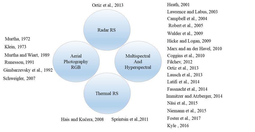
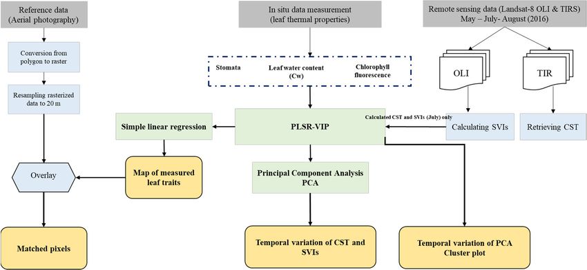
Remote Sens. 2019, 11, 398 9 of 23

which meant summer conditions. Therefore, the following formula was used to estimate the mean
atmospheric temperature [81,93]:
 Ƭa = [16.0110 + 0.92621 × (T0)] − 273.15 (7)
where Ta is the mean atmospheric temperature in degrees Celsius, and T0 is the surface air
temperature in Kelvin. Data on air temperature were obtained from the Waldhäuser weather station.
 Finally, the mono-window algorithm was employed to retrieve canopy surface temperature over
the study area, as follows:
 CST = (A × (1 – C – D) + [B × (1 – C – D) + C+D] × Bt – D × Ta) / C (8)
where CST is the canopy surface temperature in degrees Celsius, Bt which is the effective temperature
viewed by the satellite under an assumption of unity emissivity in degrees Celsius, and Ta is the
mean atmospheric temperature in degrees Celsius. In addition, the parameters A and B have
standard values proposed by Qin, Karnieli and Berliner [81] which are −67.355351 and 0.458606,
respectively, while the parameters C and D are obtained using the following formulae:
 C=ɛ×Ƭ (9)
and
 D= (1 – Ƭ ) × [1 + (1 − ɛ) × Ƭ ] (10)
where ɛ is the emissivity estimated from Equation (3), and Ƭ is the atmospheric transmittance.

2.4. Statistical Analysis
 To fulfil the objective of this research, three statistical analyses were employed, namely,
statistical significance test (Student’s t tests), partial least squares regression (PLSR), and principal
components analysis (PCA). The Student’s t tests were used to assess the impact of bark beetle
infestation at the green attack stage on the measured leaf traits (foliar stomatal conductance,
chlorophyll fluorescence, and water content) and remote sensing data (SVIs and CST). Next, to
identify the key SVIs for estimating the studied leaf traits (foliar stomatal conductance, chlorophyll
fluorescence, and water content) variable importance in projection (VIP) was calculated from the
PLSR analysis. The VIP scores are useful in understanding X space predictor variables (SVIs and CST)
that best explain dependent (Y) variables (leaf traits). The “VIP method selects those X variables that
contribute most to the underlying variation in the X variables. This includes the variation not related
to y, but describing interferences, that is so-called orthogonal variation.” [94] To achieve this, PLSR
analysis was employed. The PLSR “is a regression method that takes into account both the variance
of the dependent and the predictor variables. It specifies a linear relationship between a set of
dependent (Y) variables (leaf traits) and a set of predictor (X) variables.” (CST and SVIs) [95]. The
PLSR was used for the Landsat-8 image captured in July 2016, as it matched the time of field data
collection. Three independent PLSR models were built for each leaf trait separately as well as for each
sample group (green attacked and healthy samples). In general, a VIP score > 1 unit indicates that the
contribution of the variable (CST or SVI) was significant, and the greater the VIP value, the larger is
the contribution of the variable to the model [96].
 Moreover, to investigate the potential of separating healthy plots from infested ones in a 2-D
space, the clustering method using PCA was employed. In other words, PCA was used to determine
the importance of each SVI for discriminating between healthy and infested plots during all three
months considered in this study. PCA is an unsupervised technique and has been successfully used
in many remote sensing studies as a data reduction approach [97]. The mean centring and unit
variance producer were used to preprocess the data. The SVIs (those having a VIP score higher than
one for both healthy and infested sample plots) were treated as independent variables, and for each
image date considered in this study, two PCA models were built as follows: (a) a PCA model
including all selected SVIs and CST (VIP > 1); (b) a PCA model including only SVIs. This step is
essential because it allows us to understand and identify the most effective SVIs in terms of making
a significant contribution to discriminating healthy from freshly infested spruce plots (Figure 3).

Remote Sens. 2019, 11, 398 10 of 23

 From the selected SVIs, those that have VIP > 1, a box plot technique was used to explore the
temporal variation between healthy and infested plots for all three months considered in this study.
The values of SVIs and CST were normalized between 0 and 1 using the MinMax normalisation
method.

2.5. Mapping Bark Beetle Green Attack Infestation
 To generate the map of bark infestation, we considered the SVI with the highest VIP score as the
most important variable to estimate studied leaf traits. Linear regression was used to generate maps
of the measured leaf traits (foliar stomatal conductance, chlorophyll fluorescence, and water content),
and the generated maps of leaf traits were used as a proxy to produce a map of bark beetle green
attack. To do this, we classified the produced maps using the range of the leaf traits from the field
(Table 3). The final map contains three classes corresponding to the stress intensity in each trait.
Following this, to validate the generated map of infestation, ancillary vector-based reference data of
the green attacked areas in 2016 were obtained from the Bavarian Forest National Park (BFNP)
administration (Abdullah et al., 2018b). The flight on 11 Jun 2017 documented new dead wood (grey
attack stage) from the previous year 2016, with reference data collected from airborne colour-infrared
(VIS and NIR) aerial images (CIR) with 0.1 m spatial resolution. Full details about the processing and
interpretation of the aerial photography in the BFNP can be found (Heurich et al., 2009; Lausch et al.,
2013a). The reference data (ground truth) were in the form of polygons and were rasterised into 30
m × 30 m grid cells to match with the produced maps from Landsat-8 SVI. In total, 417 pixels were
used as the ground truth data. Furthermore, land cover data obtained from the national park
administration were used to mask out non-spruce stands and young stands. This is because bark
beetles only infest old and mature Norway spruce (Picea abies (L.) Karst). The masked land cover was
overlaid on the classified leaf traits maps in this study (Figure 3). Finally, the total number of pixels
(ground truth) located within each (stress class) were extracted and calculated.

 Table 3. Stress level categories classified using the range of the leaf traits (leaf water content, stomatal
 conductance, and chlorophyll fluorescence) from the field, in the Bavarian Forest National Park, July
 2016.

 Severely stressed Moderately stressed Healthy
 Leaf water content (g/cm2) 0.0145
 Stomatal conductance (mmol/m2s) 120
 Chlorophyll fluorescence ratio 1.25

 Figure 3. The framework of the research methodology.

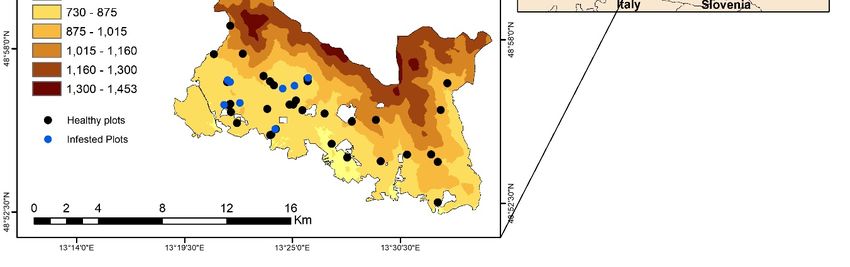
Remote Sens. 2019, 11, 398 11 of 23

3. Results

3.1. The Importance of CST versus SVIs to Estimate Measured Leaf Properties
 Infestation by bark beetle caused substantial changes in all studied leaf traits during the green
attack stage. The result of the Student’s t test demonstrated a significant difference (p < 0.05) between
healthy and infested leaves for all the studied leaf traits (chlorophyll fluorescence, leaf water content,
and stomatal conductance) (Figure 4). Furthermore, as can be seen from Figure 5, the VIP scores show
that CST significantly contributes to the estimation of studied leaf traits (chlorophyll fluorescence,
water content, and stomatal conductance) for both healthy and infested plots. However, among the
SVIs only five out of 23 had a VIP score above one for both healthy and infested sample plots; these
five indices are CIgreen, CVI, CI, NLI, and BGI (Figure 5). The single bands of Landsat-8 showed the
lowest VIP score for all measured leaf traits.

 Figure 4. Distribution of measured leaf traits for healthy and infested needles, in the Bavarian Forest
 National Park, July 2016. There is a significant difference (p < 0.05) in all measured leaf traits between
 healthy and infested samples.

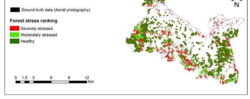
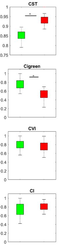
Remote Sens. 2019, 11, 398 12 of 23

 Figure 5. PLSR variable importance in the projection (VIP) for predictor (CST and SVIs) and response
 variables (measured leaf traits) in the Bavarian Forest National Park, July 2016 (the vertical black line
 represents VIP ≥ 1).

3.2. Temporal Response of CST and SVIs under Spruce Bark Beetle Infestation
 To assess the temporal variation of the CST and those SVIs that obtained a VIP score > 1, we
studied the boxplots for all three months considered in this study. Figure 6 shows a comparative
time-series of CST and SVIs for healthy and infested sample plots. As can be seen from this figure,
the CST in infested and healthy plots differ from the SVIs by exhibiting increased temperature from
the beginning of the infestation in May, whereas almost all other indices show no differences between
healthy and infested plots. Similarly, in July, when the infestation is still at its early stage (green
attack), CST shows high potential for discriminating between healthy and infested sample plots.
However, in August, when the infested plots entered into the advanced stage (in which the infested
trees developed stress symptoms by turning their needles’ colour from green to yellow to red-brown
and can be detected by the human eye), CST as well as CIgreen, NLI, and BGI are significantly
different (p < 0.05) between healthy and infested plots.
 The selected SVIs, which had a VIP value > 1 (CST, CIgreen, CVI, CI, NLI, and BGI) have been
used to build the PCA model. As shown in Figure 7, in May, when the infestation is in its early stage,
there is an apparent overlap and mixed scattering between healthy and infested sample plots when
SVIs were applied in the model. However, in July and August, when CST is included into the model,
the majority of healthy plots tend to be on the negative side of PC1, while the infested plots are
relatively scattered on the positive side of PC1. In general, we observed distinct improvement to
differentiate between healthy and infested plots when both CST and SVIs were used to build the PCA
model.

3.3. Mapping Bark Beetle Green Attack and Validation
 As shown in Figure 5, CST recorded the highest VIP score in all measured leaf traits, and
therefore we considered it as the most important variable for predicting studied leaf traits. The CST
was then used to estimate leaf traits (foliar stomatal conductance, chlorophyll fluorescence, and water
content) and generate maps using the SLR model (Table 4). Following this, based on the defined
threshold value (Table 3), stress maps were generated using leaf traits’ data. These maps were then
overlaid with ground truth reference data (417 pixels) to calculate those pixels located within each
stress class. Figure 8 and Table 5 depict those areas (pixels) that were located in each class. As can be
seen from Table 5, 274 pixels out of 417 (66%) from ground truth data were located with the severely
stressed class; following this, 89 (21%) pixels were located in the moderately stressed class and the
remaining 54 (13%) pixels where located within the healthy class .

 Table 4. Regression equations between canopy surface temperature (CST) and measured leaf
 properties.

 Equation No. Regression equations
 1 Leaf water content = −0.0004 CST + 0.0203
 2 Stomatal conductance = −6.4377 CST + 255.66
 3 Chlorophyll fluorescence = −0.0264 CST + 1.68

Remote Sens. 2019, 11, 398 13 of 23

 May July August

 Figure 6. Temporal variation of the SVIs and CST (VIP > 1) for healthy and green attacked sample
 plots in the Bavarian Forest National Park. Green and red boxes represent healthy and infested plots,
 respectively. A * indicates the significant difference between healthy and infested plots obtained using
 Student’s t tests.

Remote Sens. 2019, 11, 398 14 of 23

 A B
 Figure 7. Cluster plots based on the first two principal components (PCs), blue squares and red circles
 represent healthy and infested plots, respectively. (A) Cluster plots based on all spectral indices VIP
 > 1 including CST, and (B) cluster plots based on all spectral indices VIP > 1 excluding CST.

 Table 5. Assessment of the generated map using reference data obtained from aerial photography.

 Forest stress classes Pixels correctly matched
 Severely stressed 274
 Moderately stressed 89
 Healthy 54
 Reference pixels (aerial photography) = 417 pixels (30m).

Remote Sens. 2019, 11, 398 15 of 23

 Figure 8. The map showing the distribution of Norway spruce stands under different stress levels in
 the Bavarian Forest National Park, July 2016. The map was produced using canopy surface
 temperature and measured leaf traits (foliar stomatal conductance, chlorophyll fluorescence, and
 water content).

4. Discussion
 In the present study, for the first time, we assessed the potential of CST and SVIs to discriminate
between healthy and green-attacked trees by European spruce bark beetle (Ips typographus, L.). The
results confirmed the superiority of CST in discriminating subtle differences between healthy and
infested trees, compared to other utilised SVIs at different stages of bark beetle attack. Furthermore,
all three considered leaf traits in this study exhibited significant differences (p < 0.05) between the
two sample groups (healthy and infested), and CST was found to be an essential indicator (VIP > 1)
to estimate them.
 Of all 23 remote sensing variables (CST, SVIs, and single bands) used, the variable importance
in projection (VIP > 1) showed that CST was by far the best at estimating studied leaf traits (Figure
5). This result reaffirms findings by [24], who used TIR data obtained fixed-wing UAVs to study
thermal water stress over the peach trees. Moreover, apart from the importance of CST in estimating
leaf properties, we found that CST better discriminates between infested and healthy trees than other
SVIs. In July and August, CST was significantly higher (p < 0.05) for the infested plots than for healthy
ones (Figure 6). For example, in May, just at the beginning of the infestation, a slightly higher CST
was observed for the infested plots, whereas the SVIs showed no difference between the two groups.
According to bark beetle phenology studies, the flight activity of bark beetles and their successful
attack on living trees starts in late spring when the air temperature reaches 16.5 °C [9,98]. The new
insight offered by this result is the potential of CST to detect the subtle changes induced by bark
beetles at this stage is quite important and promising. Likewise, in July, when the infestation had
progressed, and the infested trees were completely stressed, CST maintained its sensitivity in
differentiating between healthy and green-attacked sample plots (Figure 6). It is well-known that
physiological factors, such as plant water content, can control the temperature of plants through the

Remote Sens. 2019, 11, 398 16 of 23

stomatal transpiration process [35]. Therefore, the distinct variation in CST between healthy and
infested plots is attributed to differences in the measured leaf traits, in particular, leaf water content.
As depicted in Figure 4, the amount of water content was significantly lower (p < 0.05) in the infested
plots than in the healthy ones. This may be attributed to the spores of fungi and the drilling activities
of the beetle itself that affect the living cells in the phloem and xylem and, therefore, disrupt the flow
of water and cause stomatal closure in infested trees [21]. This result further confirms our earlier
finding [99] showing a decrease of foliar biochemical properties (chlorophyll and nitrogen
concentration) in trees infested by bark beetles (I. typographus, L.) at the green attack stage. Likewise,
our findings are in agreement with [22], who studied the impact of a similar species (the mountain
pine beetle, Dendroctonus spp.) on leaf water content using hyperspectral data. Infested trees tend to
close their stomata to prevent further water loss and hydraulic failure [100]. This stomatal closure
will temporarily offset xylem cavitation and cause damage to the photosynthetic apparatus [101].
However, this behaviour leads to other physiological changes in the infested trees, such as a decrease
in the transpiration cooling process and, therefore, an increase in leaf surface temperature. Over time,
this will affect the process of photosynthesis and cause a change in foliar colour [102]. These findings
match those observed in earlier studies that the TCI index retrieved from the Landsat 7 ETM thermal
band could detect areas under mountain pine beetle (Dendroctonus spp.) green attack [28].
 In August, when the infestation had progressed and the subsequent degradation of the needles
could be observed in the field (the infested trees developed stress symptoms by turning their needles’
colour from green to yellow to red-brown), the variation of SVIs became more evident between
healthy and infested plots. CST, Cigreen, NLI and BGI were shown to have the potential to detect the
infested trees at that time. However, for effective management, identifying infested trees at that stage
is too late, because the beetles will have already left the infested trees, and logging operations will
not have any effect on the population dynamics of the beetles at that time anymore [9,20,103].
 In addition to the temporal variation, we also observed that CST improved discrimination
between healthy and infested plots when using PCA analysis for all dates considered in this study
(Figure 7). In May, when the PCA model was built based on optical data only, the two groups of
sample plots had mixed scattering and exhibited an apparent overlap, whereas, when CST was
included into the model the healthy plots were separated from the infested ones. This indicates the
increased sensitivity of Landsat-8 TIR data to changes at canopy level induced by bark beetle at a
very early stage in May. One possible reason for such sensitivity of CST to spruce bark beetle
infestation in May could be due to the nature of spruce bark beetle outbreaks, which generally occur
over the course of several years. In other words, the healthy trees are always surrounded by other
healthy trees, while, for infested trees in most cases, the infestation occurs close to the previous year’s
infestation [104]. Therefore, the open areas and dead trees around newly infested trees can lead to an
increase in surface temperature. To confirm this, we further analysed and calculated the CST for
different habitat types in the landscape. To do this, a habitat map obtained from the national park
administration was used to extract the CST for each habitat type [105]. As can be observed from
Figure 9, the results revealed that clear-cut areas, followed by lying dead-wood and standing dead-
wood areas, had the highest CST for all three months. In contrast, mixed stands showed the lowest
CST. This is supported by Peterson et al. [106] who found that forest structure (i.e. canopy closure) is
negatively correlated with simulated thermal data from the Thematic Mapper Simulator (TMS).
 Similarly, Junttila et al. [107] and Hais and Kučera [27] have shown that higher surface
temperatures were detected in dead-wood stands and clear-cut areas, respectively. Furthermore, a
water body had the lowest CST, which supports the hypothesis that more moisture in healthy tree
needles decreased their surface temperature. This also corresponded with our in situ measurements
that showed green-attacked trees had lower water content and more closed stomata than healthy
trees (Figure 4). The clear-cut area and dead-wood stands had no foliage and, thus, no leaf surface
area for evapotranspiration. This resulted in higher canopy temperatures in the cleared and dead-
wood stands than in intact stands.

Remote Sens. 2019, 11, 398 17 of 23

 Figure 9. Mean canopy surface temperature over different habitat classes in the Bavarian Forest
 National Park, 2016. The graph shows that standing dead-wood, lying dead-wood, clear-cut, and
 rocky areas recorded high surface temperature comparing to other forest classes.

 Moreover, an equally significant aspect of CST was found when used to estimate measured leaf
traits (foliar stomatal conductance, chlorophyll fluorescence, and water content) and producing the
stress map for the study area (Figure 8). The stress map highlighted the sensitivity of CST for
detecting canopies that are stressed by bark beetle green attack. In general, the majority (66%) of
ground truth data were located within the severely stressed class. However, 13% where falsely
located in the healthy class (Table 5). Consequently, CST derived from Landsat-8 TIR data might be
used to generate hotspot maps of stressed areas within the forest that show high potential areas of
bark beetle green attack. Such maps can provide valuable information to the forest management
practice when they aim to control this species and preclude a mass outbreak. Furthermore, such maps
can also be used to improve the bark beetle modelling community. For example, in our study and the
previous studies by [27] the highest temperature was observed over the dead-wood stands. Such
information on the dead-wood stands combined with the less reliable information from green
attacked areas can be used to improve the accuracy of predisposition models [108]

5. Conclusions
 The results of this study showed the potential of CST retrieved from the Landsat 8 TIR band to
detect early-stage bark beetle infestation. We further found that the infestation at the green attack
stage affected the leaf stomatal conductance, chlorophyll fluorescence, and water content. The CST
has the highest VIP value for estimating all three leaf traits measured in this study for July. In
addition, we found that CST maintained its sensitivity for monitoring and detecting bark beetle
infestation before, during and after infestation. In conclusion, our key concept is that we show for the
first time that satellite TIR data has a high potential to detect bark beetle green attack and examining
the link between the leaf traits and thermal remote sensing data is an important step that further
improves our understanding of the relationship between Earth observation data and plant traits for
forest areas under bark beetle green attack. It is important to note that TIR images obtained from
Landsat-8 are the only available satellite images that provide data at 30 m spatial resolution.
However, the original data were acquired at 100 m, so the actual footprint of the pixel is larger.
Therefore, further research investigating different TIR data with higher spectral and spatial
resolution, such as TIR from airborne hyperspectral measurements, may improve the use of thermal
imagery for bark beetle green attack detection in Norway spruce forests.
Author Contributions: H.A., R.D., A.K.S., and M.H. conceived and designed the experiment. H.A. analyzed the
data and wrote the manuscript. All authors contributed to editing of the manuscript.

Remote Sens. 2019, 11, 398 18 of 23

Funding: This research received financial support from the EU Erasmus Mundus Salam-2 and was co-founded
by Natural Resources Department, Faculty of Geo-Information Science and Earth Observation (ITC), University
of Twente, the Netherlands.

Acknowledgements:. The author’s thanks the Bavarian Forest National Park staff for approving access to the
test site and providing field and camping facilities. The authors extend their appreciation for the great support
during the laboratory measurements from the GeoScience Laboratory at ITC Faculty, University of Twente.

Conflicts of Interest: The authors declare no conflict of interest.

References
1. Morris, J.L.; Cottrell, S.; Fettig, C.J.; Hansen, W.D.; Sherriff, R.L.; Carter, V.A.; Clear, J.L.; Clement, J.;
 DeRose, R.J.; Hicke, J.A.; et al. Managing bark beetle impacts on ecosystems and society: Priority questions
 to motivate future research. J. Appl. Ecol. 2017, 54, 750–760.
2. Tchakerian, M.D.; Coulson, R.N. Ecological Impacts of Southern Pine Beetle; Coulson, R.N., Klepzig, K.D., Eds.;
 Southern Pine Beetle II. Gen. Tech. Rep. SRS-140; US Department of Agriculture Forest Service, Southern
 Research Station: Asheville, NC, USA, 2011; Volume 140, pp. 223–234.
3. Schelhaas, M.J.; Nabuurs, G.J.; Schuck, A. Natural disturbances in the european forests in the 19th and 20th
 centuries. Glob. Chang. Biol. 2003, 9, 1620–1633.
4. Eidmann, H. Impact of bark beetles on forests and forestry in sweden. J. Appl. Entomol. 1992, 114, 193–200.
5. Pasztor, F.; Matulla, C.; Rammer, W.; Lexer, M.J. Drivers of the bark beetle disturbance regime in alpine
 forests in austria. For. Ecol. Manag. 2014, 318, 349–358.
6. Seidl, R.; Rammer, W.; Jäger, D.; Lexer, M.J. Impact of bark beetle (ips typographus l.) disturbance on timber
 production and carbon sequestration in different management strategies under climate change. For. Ecol.
 Manag. 2008, 256, 209–220.
7. Lehnert, L.W.; Bässler, C.; Brandl, R.; Burton, P.J.; Müller, J. Conservation value of forests attacked by bark
 beetles: Highest number of indicator species is found in early successional stages. J. Nat. Conserv. 2013, 21,
 97–104.
8. Müller, J.; Bütler, R. A review of habitat thresholds for dead wood: A baseline for management
 recommendations in european forests. Eur. J. For. Res. 2010, 129, 981–992.
9. Wermelinger, B. Ecology and management of the spruce bark beetle ips typographus—A review of recent
 research. For. Ecol. Manag. 2004, 202, 67–82.
10. Raffa, K.F.; Grégoire, J.-C.; Staffan Lindgren, B. Chapter 1 - natural history and ecology of bark beetles. In
 Bark beetles, Vega, F.E.; Hofstetter, R.W., Eds. Academic Press: San Diego, 2015; pp 1-40..
11. Niemann, K.O.; Visintini, F. Assessment of Potential for Remote Sensing Detection of Bark Beetle-Infested Areas
 during Green Attack: A Literature Review; Natural Resources Canada, Canadian Forest Service, Pacific
 Forestry Centre, Victoria, BC, Canada, 2005.
12. Wulder, M.A.; White, J.C.; Bentz, B.; Alvarez, M.F.; Coops, N.C. Estimating the probability of mountain
 pine beetle red-attack damage. Remote Sens. Environ. 2006, 101, 150–166.
13. Coulson, R.N.; Amman, G.D.; Dahlsten, D.L.; DeMars, C., Jr.; Stephen, F. Forest-bark beetle interactions:
 Bark beetle population dynamics. In Integrated Pest Management in Pine-Bark Beetle Ecosystems; John Wiley
 & Sons: New York, NY, USA, 1985; pp. 61–80.
14. Wulder, M.A.; Dymond, C.C.; White, J.C.; Leckie, D.G.; Carroll, A.L. Surveying mountain pine beetle
 damage of forests: A review of remote sensing opportunities. For. Ecol. Manag. 2006, 221, 27–41.
15. Filchev, L. An Assessment of European Spruce Bark Beetle Infestation Using WorldView-2 Satellite Data.
 In Proceedings of 1st European SCGIS Conference with International Participation Best Practices:
 Application of GIS Technologies for Conservation of Natural and Cultural Heritage Sites‖ (SCGIS-
 Bulgaria, Sofia), Sofia, Bulgaria, 21–23 May 2012; pp. 9–16
16. Franklin, S.E.; Wulder, M.A.; Skakun, R.S.; Carroll, A.L. Mountain pine beetle red-attack forest damage
 classification using stratified landsat tm data in british columbia, canada. Photogramm. Eng. Remote Sens.
 2003, 69, 283–288.
17. Hais, M.; Jonášová, M.; Langhammer, J.; Kučera, T. Comparison of two types of forest disturbance using
 multitemporal landsat tm/etm+ imagery and field vegetation data. Remote Sens. Environ. 2009, 113, 835–845.
18. Havašová, M.; Bucha, T.; Ferenčík, J.; Jakuš, R. Applicability of a vegetation indices-based method to map
 bark beetle outbreaks in the high tatra mountains. Ann. For. Res. 2015, 58, 295–310.

Remote Sens. 2019, 11, 398 19 of 23

19. Meddens, A.J.H.; Hicke, J.A.; Vierling, L.A.; Hudak, A.T. Evaluating methods to detect bark beetle-caused
 tree mortality using single-date and multi-date landsat imagery. Remote Sens. Environ. 2013, 132, 49–58.
20. Wulder, M.A.; White, J.C.; Carroll, A.L.; Coops, N.C. Challenges for the operational detection of mountain
 pine beetle green attack with remote sensing. For. Chron. 2009, 85, 32–38.
21. Yamaoka, Y.; Swanson, R.; Hiratsuka, Y. Inoculation of lodgepole pine with four blue-stain fungi associated
 with mountain pine beetle, monitored by a heat pulse velocity (hpv) instrument. Can. J. For. Res. 1990, 20,
 31–36.
22. Cheng, T.; Rivard, B.; Sánchez-Azofeifa, G.A.; Feng, J.; Calvo-Polanco, M. Continuous wavelet analysis for
 the detection of green attack damage due to mountain pine beetle infestation. Remote Sens. Environ. 2010,
 114, 899–910.
23. Buitrago Acevedo, M.F.; Groen, T.A.; Hecker, C.A.; Skidmore, A.K. Identifying leaf traits that signal stress
 in tir spectra. ISPRS J. Photogramm. Remote Sens. 2017, 125, 132–145.
24. Berni, J.A.J.; Zarco-Tejada, P.J.; Gonzalez-Dugo, V.; Fereres, E. Remote sensing of thermal water stress
 indicators in peach. Acta Hortic. 2012, 962, 325–331
25. Jang, J.D.; Viau, A.A.; Anctil, F. Thermal-water stress index from satellite images. Int. J. Remote Sens. 2006,
 27, 1619–1639.
26. Sepulcre-Cantó, G.; Zarco-Tejada, P.J.; Jiménez-Muñoz, J.; Sobrino, J.; De Miguel, E.; Villalobos, F.J.
 Detection of water stress in an olive orchard with thermal remote sensing imagery. Agric. For. Meteorol.
 2006, 136, 31–44.
27. Hais, M.; Kučera, T. Surface temperature change of spruce forest as a result of bark beetle attack: Remote
 sensing and gis approach. Eur. J. For. Res. 2008, 127, 327–336.
28. Sprintsin, M.; Chen, J.M.; Czurylowicz, P. Combining land surface temperature and shortwave infrared
 reflectance for early detection of mountain pine beetle infestations in western canada. J. Appl. Remote Sens.
 2011, 5, 053566.
29. Ullah, S.; Skidmore, A.K.; Ramoelo, A.; Groen, T.A.; Naeem, M.; Ali, A. Retrieval of leaf water content
 spanning the visible to thermal infrared spectra. ISPRS J. Photogramm. Remote Sens. 2014, 93, 56–64.
30. Buitrago, M.F.; Groen, T.A.; Hecker, C.A.; Skidmore, A.K. Changes in thermal infrared spectra of plants
 caused by temperature and water stress. ISPRS J. Photogramm. Remote Sens. 2016, 111, 22–31.
31. Neinavaz, E.; Darvishzadeh, R.; Skidmore, A.K.; Groen, T.A. Measuring the response of canopy emissivity
 spectra to leaf area index variation using thermal hyperspectral data. Int. J. Appl. Earth Obs. Geoinf. 2016,
 53, 40–47.
32. Kümmerlen, B.; Dauwe, S.; Schmundt, D.; Schurr, U. Thermography to measure water relations of plant
 leaves. In Handbook of Computer Vision and Applications; London: Academic Press 1999; Volume 3, pp. 763–
 781.
33. Fabre, S.; Lesaignoux, A.; Olioso, A.; Briottet, X. Influence of water content on spectral reflectance of leaves
 in the 3–15μm domain. IEEE Geosci. Remote Sens. Lett. 2011, 8, 143–147.
34. Xu, H.; Zhu, S.; Ying, Y.; Jiang, H. In Early detection of plant disease using infrared thermal imaging, Optics for
 Natural Resources, Agriculture, and Foods, 2006; International Society for Optics and Photonics: p 638110.
35. Oerke, E.; Steiner, U.; Dehne, H.; Lindenthal, M. Thermal imaging of cucumber leaves affected by downy
 mildew and environmental conditions. J. Exp. Bot. 2006, 57, 2121–2132.
36. Ni, Z.; Liu, Z.; Huo, H.; Li, Z.-L.; Nerry, F.; Wang, Q.; Li, X. Early water stress detection using leaf-level
 measurements of chlorophyll fluorescence and temperature data. Remote Sens. 2015, 7, 3232–3249.
37. Aldea, M.; Hamilton, J.G.; Resti, J.P.; Zangerl, A.R.; Berenbaum, M.R. Indirect effects of insect herbivory on
 leaf gas exchange in soybean. Plant Cell Environ. 2005, 28, 402–411.
38. Moller, M.; Alchanatis, V.; Cohen, Y.; Meron, M.; Tsipris, J.; Naor, A.; Ostrovsky, V.; Sprintsin, M.; Cohen,
 S. Use of thermal and visible imagery for estimating crop water status of irrigated grapevine. J. Exp. Bot.
 2007, 58, 827–838.
39. Hunt, E.R.; Rock, B.N. Detection of changes in leaf water content using near-and middle-infrared
 reflectances. Remote Sens. Environ. 1989, 30, 43–54.
40. Kim, Y.; Still, C.J.; Hanson, C.V.; Kwon, H.; Greer, B.T.; Law, B.E. Canopy skin temperature variations in
 relation to climate, soil temperature, and carbon flux at a ponderosa pine forest in central oregon. Agric.
 For. Meteorol. 2016, 226–227, 161–173.