UNMIXING RIVER SEDIMENTS FOR THE ELEMENTAL GEOCHEMISTRY OF THEIR - EARTHARXIV
←
→
Page content transcription
If your browser does not render page correctly, please read the page content below
Unmixing river sediments for the elemental geochemistry of their
                                                                                       source regions
                                                                                         Submitted, non-peer reviewed manuscript, compiled April 15, 2021

                                                                           ∗
                                                            Alex G. Lipp1 , Gareth G. Roberts1 , Alexander C. Whittaker1 , Charles. J. B. Gowing2 , and Victoria M. Fernandes1
                                                                                    1
                                                                                      Department of Earth Sciences and Engineering, Imperial College London, UK
                                                                               2
                                                                                   Centre for Environmental Geochemistry, British Geological Survey, Keyworth, UK

                                                                                                                     Abstract
                                                                 The geochemistry of river sediments is routinely used to obtain information about geologic and environmental
                                                                 processes occurring upstream. For example, downstream samples are used to constrain chemical weathering
                                                                 and physical erosion rates, as well as the locations of mineral deposits or contaminant sources. Previous work
                                                                 has shown that, by assuming conservative mixing, the geochemistry of downstream samples can be reliably
                                                                 predicted given a known source region geochemistry. In this study we tackle the inverse problem and ‘unmix’
                                                                 the composition of downstream river sediments to produce geochemical maps of drainage basins (i.e., source
                                                                 regions). The scheme is tested in a case study of rivers draining the Cairngorms, UK. The elemental geochemistry
Manuscript submitted for publication in Geochemistry,

                                                                 of the < 150 µm fraction of 67 samples gathered from the beds of channels in this region is used to invert for
                                                                 concentrations of major and trace elements upstream. We solve this inverse problem using the Nelder-Mead
                                                                 optimisation algorithm and by seeking only spatially smooth maps. The best-fitting source region geochemistry

                                                                                                                                                                                                   Preprint doi: YYYYYYYYYYYYYYYYYY
                                                                 for 20 elements of different affinities (e.g., Be, Li, Mg, Ca, Rb, U, V) is assessed using independent geochemical
                                                                 survey data. The inverse approach makes reliable predictions of the major and trace element concentration in
                                                                 first order river sediments. We suggest this scheme could be a novel means to generate geochemical baselines
              Geophysics, Geosystems

                                                                 across drainage basins and within river channels.

                                                        Keywords Sedimentary geochemistry · Inverse modelling · Mixing · Geochemical mapping · Fluvial Geomorphology

                                                        1    Introduction                                                     River sediment geochemistry is also widely used as a medium
                                                                                                                              for geochemical surveys which provide valuable data for mineral
                                                                                                                              resource exploration, environmental monitoring and wider geo-
                                                        Sediments contained in river channels are the products of phys-       logic understanding (Garrett et al. 2008). The understanding of
                                                        ical and chemical weathering of rocks outcropping in the up-          river sediment geochemistry is therefore also significant from an
                                                        stream drainage basin (Weltje and Eynatten 2004; Weltje 2012;         applied and economic geochemistry perspective. As sediments
                                                        Caracciolo 2020). During transport, sediment geochemistry             in streams integrate the geochemistry of their entire catchment,
                                                        is also altered by processes including weathering, sorting and        sampling them is a more resource efficient way to survey large
                                                        cation-exchange (Bouchez et al. 2011, 2012; Tipper et al. 2021).      areas than sampling, for instance, soils or outcropping rocks. De-
                                                        As fluvial sediments can be transported on relatively long            pending on practical constraints however, the size of the sampled
                                                        timescales, of order 102 − 103 yr, their geochemistry repre-          catchment can vary over orders of magnitude. For example, the
                                                        sents a spatially and temporally integrated signal of catchment       National Geochemical Survey of Australia samples catchments
                                                        processes (Repasch et al. 2020). They are therefore frequently        with areas ∼ 5000 km2 , whereas the analogous national survey
                                                        studied to understand the rates and location of chemical weath-       of the UK typically samples catchments with upstream area gen-
                                                        ering, physical erosion and sediment transport (e.g., Canfield        erally less than 100 km2 (Caritat and Cooper 2016; Johnson et al.
                                                        1997; Gaillardet et al. 1999; Riebe et al. 2003; Viers et al. 2009;   2018b). Understanding precisely how the geochemical signal of
                                                        Garzanti et al. 2012; Lupker et al. 2012, 2013; Garzanti et al.       source regions propagates downstream in sediments, and how it
                                                        2014; Schneider et al. 2016; Ercolani et al. 2019). However,          can be recovered from samples downstream, would allow better
                                                        given that geochemical mixing, in-transit modification or selec-      understanding of the trade-offs involved in surveying catchments
                                                        tive deposition may take place, the extent to which downstream        of different areas. This in turn would better inform subsequent
                                                        river sediment geochemistry contains the desired source region        sampling campaigns.
                                                        signal remains challenging to quantify. An objective scheme
                                                        which translates downstream sediment geochemistry into that
                                                        of the corresponding upstream source-region is therefore desir-       1.1   Study design
                                                        able. Such a scheme would produce predictions of the upstream
                                                        geochemistry which can be used investigate controls on Earth          Our study design is illustrated by the schematic in Figure 1.
                                                        surface processes, but without the unwanted effects of mix-           Consider a river catchment that contains three geochemical end-
                                                        ing. Moreover, such a scheme would allow the effects of other         members which could correspond to, e.g., lithologic units. These
                                                        proposed in-transit processes (e.g., weathering in-transit) to be     endmembers are represented as the red, green and blue areas in
                                                        quantified. Proposing and testing such an ‘unmixing’ scheme is        Figure 1. The sediment in rivers draining each of these regions
                                                        the goal of this study.                                               inherits the geochemistry of these sediment sources, as indi-

                                                                                                      *correspondence: a.lipp18@imperial.ac.uk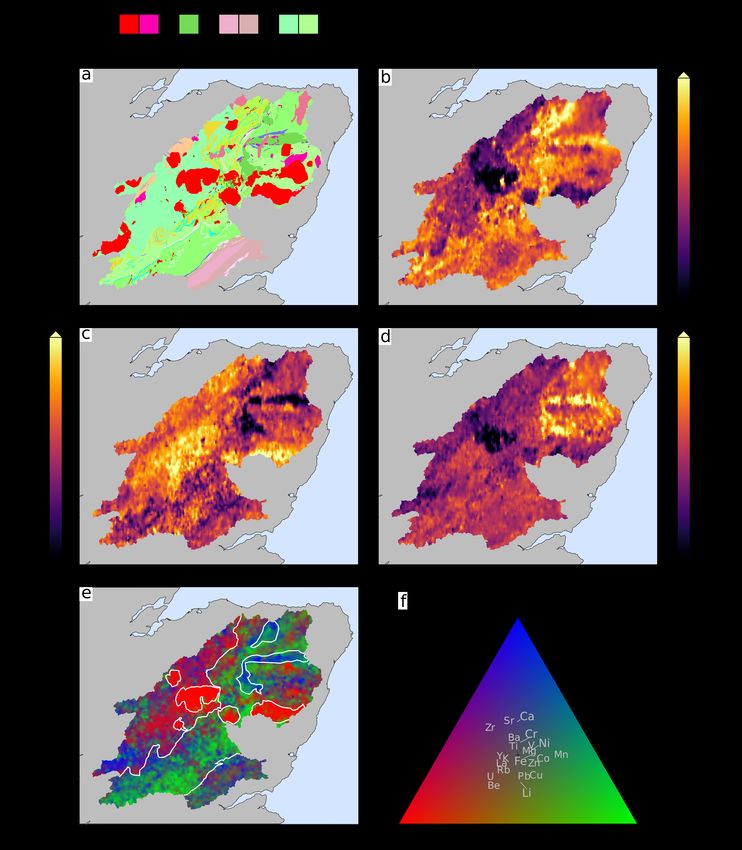
Preprint – Unmixing river sediments for the elemental geochemistry of their source regions                                          2

Figure 1: Predicting provenance: Composition of sediments in rivers and upstream sources from forward and inverse
modelling. (a) Schematic showing composition of source regions (X, Y, Z), drainage network (white lines) and composition
of sampled river sediments (white circles). In this simple scheme composition of sediment in rivers (e.g., colored pie charts)
is determined by the composition of upstream source regions. (b) Schematic shows the forward, ‘mixing’, problem when the
source region geochemistry is known and the downstream composition at sample sites is predicted (see Lipp et al. 2020). (c) The
inverse, ‘unmixing’, problem attempts to reconstruct the composition of source regions from the point observations of downstream
sediment composition, which is the focus of this study.

cated in Figure 1 by the pie charts representing the contributions   endmembers (i.e., the compositions that are being mixed) and
from each endmember. Downstream geochemistry changes as              the mixing proportions are sought, so as to explain variability
tributaries draining different sources join or the river erodes a    in a proposed mixture dataset. Weltje (1997) developed a nu-
different source region. The ‘forward’ problem, as we define it      merical solution to this general problem which has been used to
here, is to predict the composition of sediment at sample sites      model a range of different datatypes including fossil abundances,
downstream given the spatial distribution of geochemistry in         rock magnetism and grain size distributions (Dam and Weltje
source regions and a known drainage network (Figure 1b). An          1999; Weltje and Prins 2007; Dekkers 2012). In the instance
example of this forward problem was implemented and suc-             where the endmembers are assumed to be known, calculating the
cessfully validated in Lipp et al. (2020). The ‘inverse’ problem     mixing proportions is relatively straightforward, and frequently
addressed in this paper seeks unknown source region composi-         solved on an ad hoc basis or as part of a Bayesian framework
tion by inverting the known sediment compositions at the sample      (e.g., Stock et al. 2018). The unmixing problem we consider
sites downstream (Figure 1c).                                        differs in that we explicitly seek the spatial structure of both
                                                                     the endmembers and the mixture, i.e., geochemical maps of
In this manuscript we consider the ‘source region geochemistry’
                                                                     source regions and the composition of downstream river sedi-
to mean the elemental composition of river sediments in the
                                                                     ment samples, respectively. This approach is most similar to that
most upstream portion of the drainage network, i.e., first order
                                                                     developed by De Doncker et al. (2020). They sought the spatial
streams. We recognise that other definitions of source region
                                                                     pattern of erosion in a catchment through a Bayesian inverse of
geochemistry may be used, most obviously the composition of
                                                                     downstream sediment tracers. We, instead, seek the composition
the underlying bedrock lithology. We use the geochemistry of
                                                                     of source regions given mixing proportions calculated using
stream sediments as our target as opposed to the bedrock as
                                                                     drainage networks.
stream sediments have already undergone chemical weathering
on hillslopes prior to entering the drainage network. Stream
sediment geochemistry is also strongly influenced by the under-      1.2   Outline
lying bedrock (see e.g.,Kirkwood et al. 2016). Stream sediments
hence incorporate geochemical information about both lithol- In this study, we first introduce the study area in the Cairngorms,
ogy and weathering whereas bedrock can only inform about     UK, where we demonstrate the approach. We describe how 67
lithology.                                                   samples of bed material were gathered from trunk channels and
                                                             tributaries along the five major river basins in the area. An im-
Given the ubiquity of mixing in the Earth sciences, a number plementation of the forward problem for these drainage basins
of quantitative unmixing procedures have been previously de- is described in Lipp et al. (2020). We then present a quantitative
veloped. The most general case of unmixing is where both the procedure that uses the structure of drainage networks to convert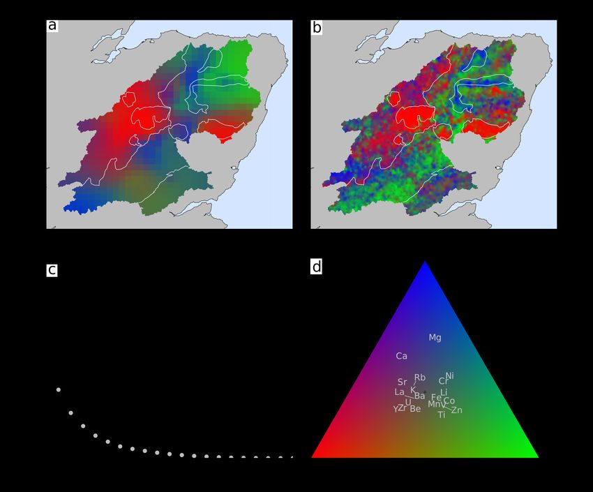
Preprint – Unmixing river sediments for the elemental geochemistry of their source regions                                           3

maps of source region geochemistry into predictions of down-        of magnesium, potassium and titanium respectively in stream
stream sediment geochemistry at sample sites. A formal inverse      sediments from the G-BASE dataset. These geochemical maps
problem is then posed, in which the unknown geochemistry of         indicate the strong relationship between stream sediment geo-
source regions is sought. We describe how this problem can be       chemistry and the underlying lithology (Figure 3a). For example,
solved by inverting downstream samples by optimisation of a         the felsic intrusions at the centre of our region are low in Mg
regularised objective function. The fidelity of predicted source    and Ti but enriched in K.
compositions generated from this inverse procedure is assessed
                                                                    We can explore the geochemical variability of the region better
by recovery of known synthetic inputs. We then present the
                                                                    using Principal Component Analysis (PCA), a multivariate tool
results of inverting real geochemical data from downstream sedi-
                                                                    frequently applied to geochemical survey data (e.g., Kirkwood
ment samples for different geochemical elements. Finally, these
                                                                    et al. 2016). PCA rotates multi-dimensional data onto a smaller
results are evaluated using independent geochemical survey data
                                                                    number of principal components (PCs) along which variance
from the study region.
                                                                    is maximised. This rotation therefore simplifies a dataset. Full
                                                                    details of this multivariate method are given in the methods.
1.3   Study area                                                    Figure 3e displays the first three PCs of 22 elements from the G-
We focus our study on five rivers draining the Cairngorms moun-     BASE dataset in a red-green-blue (RGB) ternary space (Figure
tains, Scotland, UK: Dee, Deveron, Tay, Don and Spey (Figure        3f), where the RGB channels correspond to the (normalised
2a). River sediments were extracted from these channels at          exponents of the) first, second and third PCs respectively. This
67 sample sites indicated in Figure 2b–c. Sediments within          figure therefore displays the principal geochemical domains of
these rivers have been previously analysed by Lipp et al. (2020),   the region. The first PC corresponds to relative enrichment in
where it was demonstrated that the forward problem described        felsic associated elements (e.g., U, Be, Rb) and defines the felsic
in Figure 1 can be used to make accurate predictions of down-       intrusions at the centre of the study region. The second PC
stream river geochemistry. This successful demonstration of the     corresponds to an enrichment in certain metals (e.g., Pb, Cu, Li)
forward model means that these same rivers are excellent can-       and appears to demarcate the different sedimentary units. The
didates to explore the use of inverse modelling. The region has     third PC corresponds to relative enrichment in some alkaline
also been geochemically mapped by the Geochemical Baseline          earths (Sr, Ca, Ba) and identifies the mafic intrusions in the
Survey of the Environment (G-BASE), a geochemical survey            NE of the study area. The goal of our inverse modelling is
conducted by the British Geological Survey (Johnson et al. 2005;    to reconstruct these principal geochemical domains using just
sample sites shown in Figure 2d). As a result, there is a pre-      a small number of sediment samples gathered from localities
existing independent dataset that can be used to test predictions   downstream.
from inverse modelling. We chose this region for three reasons.
First, for the UK, it has relatively high topographic relief and    2.2   Downstream sediment geochemistry
a high natural sedimentary flux. Second, a significant portion
of the region is in a protected national park limiting potential    The < 150 µm fraction of bed material was gathered from local-
anthropogenic effects. Finally, this region contains a variety of   ities on the studied rivers and their geochemistry was measured
lithologic units and substrate compositions including mafic and     following G-BASE protocols. This dataset was first reported
felsic igneous intrusions hosted within meta-sedimentary units      in Lipp et al. (2020). In total, 67 samples were gathered from
(Figure 3a).                                                        63 sample sites (Figure 2b). The sample sites divide the study
                                                                    area into a series of nested sub-catchments, which are displayed
                                                                    in Figure 2c. Sampling density means that the majority of sub-
2     Data & Methods                                                catchments have areas 200–400 km2 . In the southern portion
                                                                    of the Tay catchment lower sampling density results in sub-
2.1   Upstream source region geochemistry                           catchments with greater areas (Figure 2c).
We will test predicted source compositions using the indepen-       At four localities duplicate samples were extracted to investi-
dent G-BASE geochemical survey data. G-BASE sampled the             gate local geochemical heterogeneity. Statistical analysis of the
fine-grained, < 150 µm, fraction of low-order stream sediments      duplicate samples, reported in Lipp et al. (2020), indicated that
(i.e., those with very small upstream areas) with an average        the vast majority of the geochemical variability in these samples
sampling density of 1 per 2 km2 . These sediment samples were       reflects variation between sample sites, not local heterogeneity.
subsequently analysed for a range of geochemical analytes. In       Whilst a larger suite of elements was gathered, we focus on the
the study region this analysis was performed principally by Di-     following 22 elements, which are present in the downstream
rect Reading Optical Emission Spectrometry, with the exception      samples and were measured consistently by G-BASE in the
of uranium which was analysed by Delayed Neutron Activation.        study area: Ba, Be, Ca, Co, Cr, Cu, Fe, K, La, Li, Mg, Mn, Ni,
The sampling and geochemical analytic procedure used by G-          Pb, Rb, Sr, Ti, U, V, Y, Zn and Zr. This subset was selected so
BASE, as well as quality control measures, are described by         that predictions from the inverse model can be evaluated using
Johnson et al. (2018a,b).                                           the independent G-BASE dataset.
The G-BASE stream sediment geochemical survey, like other           The sampling procedure we used replicated the standard G-
high sample density surveys, primarily reflect geochemicals         BASE sampling protocol. This replication makes the data gath-
variations in the underlying bedrock (Everett et al. 2019). This    ered directly comparable between the two datasets. bed material
lithological control on geochemical survey data is also clearly     was extracted from the river channel by shovel and deposited
displayed in our study region. Figure 3a displays the geological    on a sieve-stack. First, a 2 cm grill was used to remove pebbles.
map of our study area. Figures 3b-d indicate the concentration      The material was then rubbed through a 2 mm and then 150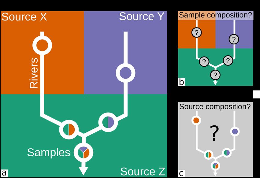
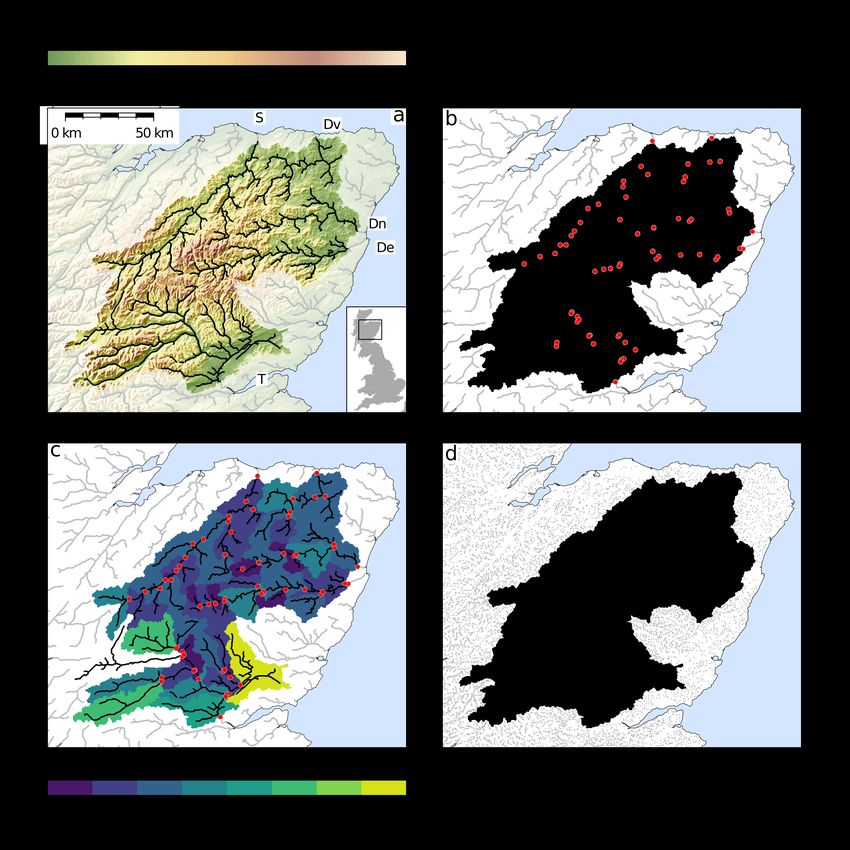
Preprint – Unmixing river sediments for the elemental geochemistry of their source regions                                   4

Figure 2: Introduction to study area: Cairngorms, UK. (a) Topography from SRTM1s digital elevation model. Transparent
overlay indicates region outside the five studied river catchments. Black lines = river channels with upstream area > 25 km2 .
Rivers labelled: S = Spey, Dv = Deveron, Dn = Don, De = Dee, T = Tay. Inset shows location of study area. (b) Location of
67 sediment sample sites (red circles) on river channels used to predict the composition of upstream source regions. (c) Unique
drainage area segments corresponding to each sample site; color indicates area of sub-catchment, which approximates effective
resolution of the inverse model (see body text). (d) Black points = G-BASE geochemical survey sample sites, which are used to
test the accuracy of predicted source region chemistry. Gray points lie outside of studied catchments.
Preprint – Unmixing river sediments for the elemental geochemistry of their source regions                                         5

Figure 3: Geology and geochemistry of Cairngorms. (a) Geologic map of studied area, reproduced with the permission of the
British Geological Survey UKRI, all rights reserved. Major lithologies indicated: FIg = Ordovician to Devonian felsic igneous
intrusions; MIg = Ordovician to Silurian mafic igneous intrusions; SR = Sedimentary rocks, mostly Devonian sandstones; MS
= Metasedimentary rocks, mostly Neoproterozoic psammites. See mapapps.bgs.ac.uk/geologyofbritain/home.html for
full geologic key. (b) Concentration of magnesium in first-order stream sediments from G-BASE survey. Note relationship to
lithology shown in panel (a) and similar spatial structure to other elements displayed in panels (c–e). (c) Potassium. (d) Titanium.
(e) Principal component map for 22 elements in G-BASE dataset following a centred log-ratio transformation (Aitchison 1983).
The first three principal components of the dataset are extracted and converted into a red-green-blue ternary space, which highlights
the major geochemical domains in the study region. White lines indicate simplified lithological map to highlight key geochemical
domains. See panel (f) for key. (f) Ternary plot showing relationship between colour, principal components and geochemistry.
Reds and greens indicate compositions that are relatively enriched in elements such as U, Be, Rb indicating felsic association and
metallic elements (e.g., Li, Pb, Cu, Co), respectively; blues indicate relative enrichment in alkaline earth elements (e.g., Ca, Sr,
Ba). The displayed principal components explain 62.1 % of the total variance.
Preprint – Unmixing river sediments for the elemental geochemistry of their source regions                                            6

µm nylon sieve into a fiberglass collecting pan. After letting      exponentials. The resulting values (which sum to one) are then
suspended sediment settle out for ∼ 15 minutes, excess water        used to weight the red, green and blue channels respectively for
was decanted, and the homogenised sediment slurry was poured        visualisation.
into a reinforced paper bag. Each paper bag was placed within a
sealed plastic bag to prevent contamination. The bagged sedi-
ment samples were air-dried until they had the consistency of       3     Forward and Inverse Modelling
modelling clay, before being freeze-dried for short-term storage
prior to geochemical analysis.                                      3.1   Forward model
The freeze-dried sediments were powderised in an agate ball mill    Here we describe the procedure to predict downstream sediment
and homogenised, and an analytical subsample taken by cone-         geochemistry given a known distribution of geochemistry and to-
quartering. For each geochemical analysis 0.25 g of powder          pography in the source-region. The forward model as described
was accurately weighted into Savillex tubes. The powders were       here has been implemented and succesfully tested for this region
digested using HF, HNO3 and HClO4 on a hotplate. Comparison         previously (Lipp et al. 2020). Let C(x, y) be the concentration
to standards indicated that some elements hosted in resistate       of some element in the sediment source regions of a drainage
minerals (e.g., Zr) were, as expected from this method, only        network, e.g., magnesium. C can be approximated by geochem-
partially digested at this stage. Post-digestion the sample was     ical surveying, e.g., Figure 3b-d. We seek to predict D which
resolubilised using HNO3 and H2 O2 , and analysed for a full        is the concentration of that same element in downstream river-
suite of elements using an Agilent 8900 Inductively Coupled         sediments at a point in a river which has an upstream drainage
Plasma Mass Spectrometer at the British Geological Survey.          area ‘A’. The concentration downstream, D, is simply the sum
                                                                    of the contributions to this element from every upstream point in
                                                                    the basin, A, normalised to the total sediment flux. If A has a spa-
2.3   Topographic data and processing
                                                                    tially varying erosion/surface-lowering rate, ∂z
                                                                                                                   ∂t , then each point
For our inverse scheme we require the drainage-network of the                         ∂z
                                                                    in A contributes ∂t × C amount of the target element, i.e., the
region to be defined. We opt to extract drainage automatically      total amount of sediment produced by that point, multiplied by
from topographic data using widely-used algorithms. Drainage        the concentration of the element in question. The total sedimen-
networks were extracted from the SRTM1s topographic dataset         tary
                                                                    R ∂zflux is the total amount of erosion occurring upstream, i.e.,
down-sampled to a square grid with resolution 200 × 200 m.                dA. Combining these relationships provides the following
                                                                     A ∂t
Prior to down-sampling the data underwent a cylindrical equal-      estimate of concentration in downstream samples
area projection centred on the study area using GMT 6.0.0 (Farr
et al. 2007; Wessel et al. 2013). Depressions in the digital ele-
                                                                                                                 ∂z
                                                                                                         Z
vation model were then filled use the ‘priority-flood’ algorithm                                 1
                                                                                        D= R                        C dA.           (1)
(Barnes et al. 2014). Subsequently, drainage networks were                                       ∂z
                                                                                                    dA       A   ∂t
                                                                                               A ∂t
extracted from this DEM using the ‘D8’ flow-routing algorithm,
which allows drainage area to be defined at every point in the      Under this formulation the concentration of element in sediment
model grid (O’Callaghan and Mark 1984). The location of             downstream can be predicted if the erosion rate and concentra-
major channels, i.e., cells with upstream area > 25 km2 are         tion can be defined at all points in the upstream region, assuming
shown in Figure 2a-c. All landscape modelling calculations          instantaneous sediment transport and no in-transit chemical mod-
were performed using the LandLab 2.2.0 package for python           ification (e.g., Sharman et al. 2019; De Doncker et al. 2020).
3.8.5 (Van Rossum and Drake 2009; Barnhart et al. 2020). The        This approach assumes that all chemical weathering happens
resulting extracted drainage networks are displayed throughout      in-situ (e.g., on hillslopes) before sediments enter the fluvial
the manuscript (e.g., Figure 2a–c).                                 system.
                                                                    An unknown in this formulation is erosion rate, ∂z/∂t. As ∂z/∂t
2.4   Principal Component Analysis                                  is required to be defined continuously across the studied region,
                                                                    a reasonable approach is to use landscape evolution models.
PCA is used in this study to investigate relationships between
                                                                    The widely-used stream power model, for example, predicts
elements and to identify spatial geochemical domains. PCA
                                                                    erosion rates using empirical relationships between slope angle,
is a very widely used technique to simplify high-dimensional
                                                                    upstream area and erosion rate (see e.g., Howard and Kerby
datasets. As geochemical datasets are compositional in nature
                                                                    1983; Tucker and Whipple 2002). In Lipp et al. (2020) the
(i.e., strictly positive data that sum to a constant) a log-ratio
                                                                    stream power model was used to predict erosion rates and hence
transformation must be applied prior to application of PCA.
                                                                    composition of sediment downstream using Equation 1 for the
In this instance we use the centred log-ratio transformation
                                                                    same data-set used here. Changing model parameters had a
(Aitchison 1983). We apply PCA to both the G-BASE datasets
                                                                    minor effect on the goodness-of-fit for downstream data. In
and our inverse solutions. We use the implementation of PCA in
                                                                    fact, spatially homogenous incision (i.e., constant ∂z/∂t) was
the scikit-learn package for python which uses singular value
                                                                    found to provide, by a small margin, the best fit to the data
decomposition to define the principal components (Pedregosa
                                                                    downstream. These results, combined with the results of tests
et al. 2011).
                                                                    in which substrate was varied, indicated that downstream geo-
To visualise three PCs simultaneously on one map we transform       chemistry was much more sensitive to the drainage network
them onto an RGB mixing ternary (e.g., Figure 3e–f) as fol-         topology and source region geochemistry. Hence, in this study
lows. The scores on the first three PCs are calculated, raised      we proceed with this assumption of homogeneous incision. The
to an exponent and then normalised by the sum of these three        validity of this assumption of spatially constant incision will be
Preprint – Unmixing river sediments for the elemental geochemistry of their source regions 7
implicitly tested when predictions from inverse modelling are 3.2.2 Data misfit
compared to independent data.
We seek the upstream geochemistry vector, C, that best explains
Under the assumption of homogenous incision (i.e., ∂z/∂t = k, the observations of concentration downstream which we repre-
where k is a constant), Equation 1 can be simplified further to sent as a vector, Dobs . This vector has length 67, equal to the
give number of observations we have made. For each observation,
there is a corresponding predicted concentration, which is sim-
1
Z ply the value of F(C) evaluated at the sample site. We represent
D(x, y) = F(C) = C dA. (2) these predictions, for a given C, as the vector F(C). We need to
|A| A formally define a metric that quantifies the difference between
This simply states that the composition of sediment downstream, the predicted, F(C), and observed, Dobs , sediment concentra-
D, is an equal area weighted mixture of the composition of tions. For this, we use the square of the Euclidean norm of the
its upstream region. In summary, Equation 2 is the forward difference between the values, after a logarithmic transform, i.e.,
model, F(C), we use to transform a spatial map of upstream
geochemistry, C(x, y), into a prediction of sediment geochem- 2
X
= log{F(C)i } − log{Dobs,i } 2 .
istry downstream, D(x, y). Figure 4 shows solutions to this log{F(C)} − log{Dobs }
forward problem. In this example the mapped concentration of i
Mg from G-BASE (Figure 3b) is used as C and input into the (3)
forward model to predict the downstream sediment concentra- We utilise the logarithmic transform prior to calculating the
tion, D = F(C). This predicted downstream concentration is misfit, again, due to the relative nature of information in compo-
shown in Figure 4a with the true observations overlain. sitional data. A visualisation of the misfit between and observed
and predicted concentrations is shown in Figure 4b.
3.2 Defining the inverse model
3.2.3 Regularisation
3.2.1 Traversing model space
This inverse problem is likely to always be underdetermined
The goal of the inverse procedure is to identify the upstream (i.e., there are fewer observations than free parameters). In the
geochemistry, C, that best fits point observations downstream. example we consider there are almost an order of magnitude
Here we describe a procedure for systematically and objectively more unknown compositions (upstream source) than known
exploring different possible values of C. We discretise C onto a compositions (downstream samples). Underdetermined prob-
grid of x × y resolution 5 × 5 km. Thus C is represented as a lems are often solved by imposing constraints on properties of
vector, C, of length equal to the number of grid-cells contained the solution, e.g., minimising roughness (Parker 1994). In this
within or overlapping our studied drainage area, which for our instance, we seek smooth geochemical maps that best fit the
chosen resolution is 601. This discrete vector can be converted composition of the 67 downstream samples. We do so by penal-
into a continuous map of geochemistry, C, by upsampling onto ising the roughness of upstream geochemistry, C. We formally
the resolution of the base DEM we use (200 × 200 m). This define roughness here as the sum of the square of the Euclidean
upsampled C can then be fed into the forward model. norms of the first derivative of C 0 in both the x and y directions,
i.e.,
Instead of seeking the vector C directly, we instead seek the
vector log(C), which we term C0 . We seek log(C) as the infor-
mation contained in geochemical data is relative, not absolute ∂C 0 2
∂C 0 2
+ . (4)
(Aitchison 1986; Pawlowsky-Glahn and Egozcue 2006). For ∂x ∂y
example, consider the change in concentration of some trace-
element from 0.01 wt% to 1 wt%. This is a significant relative To quantify the first-derivative we calculate the first discrete
change of 100 times the original value, but an absolute change difference between adjacent values of the, logarithmic, C0 grid
of only 0.99 wt%. If that same element changes in concentra- in both the x and y directions, assuming Von Neumann boundary
tion again to 2 wt%, the relative change is only two times the conditions that are equal to zero (i.e., ∂C 0 /∂x = ∂C 0 /∂y = 0).
intermediate value, much smaller than the initial change. How-
ever, the absolute change is in fact larger, i.e., 1 wt%. Given 3.2.4 Optimising the objective function
that elemental concentrations frequently traverse many orders Considering both the data-misfit and roughness constraints, the
of magnitude, our cost function must be sensitive to relative not best fitting source-region chemistry is that which minimises the
absolute changes in concentration. In logarithmic space, the first following objective function, X(C0 ):
change in concentration is correctly identified as traversing a
greater compositional distance than the second change, hence
its application here. Roughness
Data Misfit z }| {
0 2 0 2
We note that as compositional data is strictly bounded between ∂C ∂C
z }| {
2
X(C0 ) = log{F(C)} − log{Dobs } +λ2 + .
0 and some closure value (e.g., 100 %, 106 ppm etc...), the sig- ∂x ∂y
moidal logit function should be used instead of a log function.
(5)
However, given that the elements we analyse here are all gener-
ally < 10 wt%, where the logit and log functions are functionally As we, strictly speaking, seek log(C), which must be raised to
identical, we use a log function as it is computationally faster to an exponent prior to being entered into the forward model, this
calculate. is a non-linear inverse problem.Preprint – Unmixing river sediments for the elemental geochemistry of their source regions 8
a b
4.5
57.5° Misfit
Observed Mg / log10(mg kg-1)
4.0
1
1:
3.5
56.5°
||Misfit|| = ΣMisfit2 = 1.28
3.0
−5° −4° −3° −2° 3.5 4.0 4.5
Predicted Mg / log10(mg kg-1)
3.4 3.6 3.8 4.0 4.2 4.4
Sediment Mg Concentration / log10(mg kg-1)
Figure 4: Predicting chemistry downstream: Example of solving the forward problem. (a) Coloured lines show predicted
concentration (C) of magnesium along rivers generated by integrating magnesium concentrations from the G-BASE survey with
respect to distance downstream (Figure 3b; see body text). Coloured circles are 67 independent spot measurements of magnesium
concentration in river-sediments (see Lipp et al. 2020). (b) Cross-plot of observed, F(C), and predicted, Dobs , magnesium
concentration at the 67 sample sites. Black line = 1:1 relationship. Global misfit (1.28) is the summed squared differences between
the logarithm of F(C) and Dobs (see body text; e.g., double-headed arrow).
The parameter λ is the smoothness coefficient that controls the five rivers. The number of iterations required to converge to
extent to which roughness is penalised. λ is a hyper-parameter a solution is generally of the order 105 –106 depending on the
that must be manually set for each element. High values of element and λ value chosen. On the authors’ standard desktop
λ result in solutions which are spatially very smooth but fit with Intel i7 processor at 2.5 GHz this takes on the order of
the data poorly (underfitting). Conversely, very low values of 101 - 102 hours to converge. A Jupyter notebook containing
λ result in very good fits to the data but resultant maps of C python implementations all of the calculations described above
which are geologically implausible due to their spatial roughness is provided (see Data Availability Statement).
(overfitting). Hence, λ is chosen based on this trade-off between
roughness and data-misfit. We use the ‘elbow’ method of Parker
(1994), where many values of λ are tried and the optimal λ is 4 Results
chosen such that it lies at the maximum curvature of a data-misfit 4.1 Synthetic Examples
against roughness plot.
First we explore the extent to which this inverse scheme can
Assuming that there is no analytic solution for the minima of recover a known, synthetic input. Figure 5a displays a synthetic
X we minimise Equation 5 numerically. We minimise X, with source-region geochemistry for an arbitrary geochemical ele-
respect to C0 , using Gao and Han (2012)’s implementation of ment. This ‘chequerboard’ pattern has a peak-to-trough distance
the Nelder-Mead algorithm using SciPy libraries (Virtanen et al. of 40 km. From this synthetic input we then calculate the compo-
2020). The Nelder-Mead algorithm, also known as the downhill sition of downstream samples, which become the ‘observations’
simplex method, works by generating a series of multidimen- used to invert for a source composition (Equations 2 & 5). We
sional simplexes (the 2D simplex is a triangle, the 3D simplex invert 67 ‘observations’ at locations corresponding to the actual
is a tetrahedron etc.) that by a series of reflections, expansions sample locations along the Spey, Deveron, Dee, Don and Tay
and contractions brackets the minimum of the objective function rivers. If the inverse scheme is working correctly, the best fitting
with an increasingly tight radius (see e.g., Press et al. 1992). The C should approximate the input map displayed in Figure 5a.
algorithm finishes when the absolute change in the objective
function and the maximum change of any parameter at each Comparing Figure 5b to Figure 5a it is clear that the inverse
iteration cycle is less than a specified tolerance. Both these scheme is successfully able to largely recover the location and
criteria must be met for convergence. We use an absolute finish- amplitude of geochemistry in sediment source regions. We em-
ing tolerance for both X and C0 of 10−4 . As an initial starting phasise that this input was recovered using just the 67 (synthetic)
condition for C0 we assume a homogenous composition equal to observations at the sample sites (red dots in Figure 5b). The
the upstream-area weighted average composition of the samples ‘pixelation’ in Figure 5b is a result of the discretization of C,
extracted from the most downstream samples of each of the discussed above, but does not prevent the scheme from resolv-
ing the significant spatial signals. The best-fitting solution toPreprint – Unmixing river sediments for the elemental geochemistry of their source regions 9
Concentration, log10(mg/kg)
3.0 3.2 3.4 3.6 3.8 4.0
−5° −4° −3° −2° −5° −4° −3° −2°
a b
57.5° 57.5°
56.5° 56.5°
4.0
c d RMS = 0.115
3.8 57.5°
Synthetic Input, log10(mg/kg)
3.6
3.4
1
3.2
1:
56.5°
3.0
R2 = 0.712
3.2 3.4 3.6 3.8 4.0 −0.3 0.0 0.3
Inversion Output, log10(mg/kg)
0 20 40 −0.4 −0.2 0.0 0.2 0.4
Count Misfit, log10(mg/kg)
Figure 5: Predicting geochemistry upstream: An example of solving the inverse problem. In this example we test the fidelity
of the inverse model by inverting for a synthetic (i.e., completely known) source composition using real rivers and positions of
actual sample sites. (a) Synthetic elemental concentration map generated using a 2D sine function (peak to trough = 40 km).
This map was used to calculate sediment concentrations at sample sites (red circles in panel b), which were inverted for source
composition. (b) Predicted source composition calculated by inverting synthetic compositions at the 67 sample sites (red circles).
In this example smoothing parameter λ = 10−0.5 . (c) 2D histogram of observed and predicted source concentrations; the grid
resolution of observed and predicted composition is 5 × 5 km (see panel b). 1:1 relationship is shown by gray dashed line; black
solid line = linear regression. (d) Misfit between observed and predicted source composition. Color bar is discretised on intervals
equal to global RMS misfit. Misfit is highest in regions of low sample coverage (see Figure 2c). Inset shows histogram of misfits
with binwidth = global RMS misfit; Best fitting normal distribution (black curve) is shown for comparison. Analogous figures for
synthetic inputs with different input wavelengths are given in Supplementary Figure S-1.Preprint – Unmixing river sediments for the elemental geochemistry of their source regions 10
−5° −4° −3° −2° −5° −4° −3° −2°
4.0 a b
57.5° 57.5°
Concentration, log10(mg/kg)
3.8
3.6
3.4
3.2
56.5° 56.5°
3.0
4.0
c d S Dv
3.8 57.5°
Observed, log10(mg/kg)
3.6 Dn
De
3.4
3.2
56.5°
1
1:
T
2 -4
||Misfit|| = ΣMisfit = 3.04 x 10
3.0
3.0 3.2 3.4 3.6 3.8 4.0
Predicted, log10(mg/kg)
4.0
e
Concentration, log10(mg/kg)
3.9
3.8
3.7
3.6
140 120 100 80 60 40 20 0
Distance upstream from mouth, km
Figure 6: Downstream chemistry from best fitting inverse model. (a) Best fitting source region geochemistry generated by
inverting synthetic ‘samples’ shown as coloured circles in panel (b), see Figure 5b. (b) Colored lines = predicted downstream
sediment concentrations from best fitting inverse model. Filled circles = synthetic ‘observations’ that were inverted for source
composition. (c) Cross-plot of observed and predicted concentrations at each sample site (black circles). Gray dashed line = 1:1
line. (d) Coloured lines indicate locations of river long-profiles displayed in panel (e): S = Spey, Dv = Deveron, Dn = Don, De =
Dee, T = Tay. (e) Coloured lines = predicted sediment concentration from best fitting inverse model along the rivers shown in
panels (b) and (d). Colored dots show concentrations at the sample sites indicated by black crosses in panel (d).Preprint – Unmixing river sediments for the elemental geochemistry of their source regions 11
the inverse problem and the synthetic input are compared on a chemical survey dataset. Hence, the veracity of predictions
cross-plot in Figure 5c. Note that we downsample (i.e., resample from the inversion scheme can be validated using independent
onto a lower-resolution grid) the input onto the same resolution observations.
as the inverse grid using a block-mean function to allow the two
As an example, we focus first on the results for magnesium.
grids to be compared. The data lie clustered close to the 1:1
Figure 7a shows the concentration of Mg upstream that best-fits
line with an R2 of 0.71 and root-mean-square (RMS) misfit of
the composition of the 67 downstream samples. Figure 7b shows
0.20, indicating that the majority of variance is explained in an
Mg from the G-BASE database downsampled.to the resolution
unbiased manner by our model.
of the inversion grid. The two maps show the same spatial
Plotting the misfit between the synthetic input and the inverse structure. The low Mg of sediments derived from the felsic
solution spatially indicates where our scheme performs compara- intrusions in the centre-left of the region is correctly identified
tively worse. Figure 5d shows that the residuals are not randomly by the inverse solution. Similarly, the two lobes of high-Mg
distributed. This is confirmed by calculating the Moran’s I for in the upper-right of the region, corresponding to sediments
these residuals, a statistic of autocorrelation which ranges be- derived from mafic intrusions, are also correctly identified in the
tween -1 and +1. Variables with no spatial autocorrelation (i.e., best-fitting inverse model. A cross-plot of the inverse solution
spatially decorrelated) tend to have an I ∼ 0. We find that the and G-BASE data is shown in Figure 7c and confirms that our
residuals shown in Figure 5d have a Moran’s I of 0.08. Whilst inverse solution correlates with the independent dataset and
this I value is low in magnitiude (indicating a generally small clusters around the 1:1 line. We emphasise again here that
effect size) this value was greater than the expected I under the the solution displayed in Figure 7a is completely independent
null hypothesis with a p-value < 0.05 suggesting a statistically of the G-BASE survey data and calculated using only the 67
significant spatial structure. This structure in the residuals is data-points we collected downstream.
imparted by spatial changes in sampling density. In the south
The predicted downstream geochemistry, i.e., F(C), for this op-
of the studied region, the residual misfits are larger. This region
timal solution is displayed in Figure 8. Comparing the predicted
coincides with low sampling density (Figure 2c; Figure 5b).
downstream chemistry indicates that the model captures the im-
Where the sample density is more consistently high, across the
portant geochemical variability within and between drainage
rest of the region, the signal is successfully recovered.
basins. However, the model does not overfit the data which, as
Figure 6 displays how this best fitting upstream geochemistry it likely contains some random noise, is a desirable result. A
relates to the observations of geochemistry downstream. Fig- cross-plot of predicted and observed downstream geochemistry
ure 6b displays the predicted downstream geochemistry for the indicates that the model is unbiased with a regression close to
best-fitting solution displayed in Figure 5b. Overlain on this the 1:1 line, and explains 76 % of the total variability.
panel are the synthetic ‘observations’, which were inverted for
The solutions displayed in Figures 7 and 8 use a smoothing
upstream composition. Figure 6c is a cross-plot of synthetic
coefficient λ = 100.3 . This value is chosen as it lies in the
‘observed’ concentrations against the predicted concentration
‘elbow’ of the data-misfit – roughness plot shown in Figure 9a.
from the best-fitting inverse model. These points all lie clustered
Each point on this graph corresponds to the roughness and data-
on the 1:1 line indicating that the model was able to fit the down-
misfit of a solution which minimises Equation 5 for a specified
stream data well. The variation in predicted geochemistry of the
λ. Changing the λ affects the extent to which roughness or
arbitrary element as a function of downstream distance, with the
data-misfit are weighted in Equation 5. The optimum λ value
observations overlain, is shown in Figure 6e. The discrete jumps
is that which weights both factors without either dominating
displayed in the concentration profiles are caused by tributaries
the total value of the objective functions, resulting in a point
joining the main channel. The inverse solution correctly predicts
which lies in the elbow of the figure. Choosing λ values greater
‘observed’ downstream variability of sediment geochemistry.
than the optimum clearly over-smooth the solution relative to
By inputting synthetic signals with patterns of different spatial the independent G-BASE dataset resulting in a poor-fit to the
scales we can qualitatively assess the effective resolution of data (Figures 9e-f). Conversely, reducing λ allows the scheme to
our scheme. Herein we refer to the different spatial-scales of overfit the data with results which are implausible in reference
geochemical features as wavelengths. Figure S-1 displays the to the independent dataset (Figures 9b-c). λ must be calibrated
inverse results for analogous signals to Figure 5a but with differ- in this way for each element.
ent trough-to-peak distances. When the spatial structure is small
In Figure 10 we display the optimal solution to the inverse equa-
(< O(10) km) our scheme cannot resolve any spatial variability.
tion against independent data for four other elements, chosen
It is however very successful at resolving longer-wavelength
as they show a range of different chemical affinities. Calcium
spatial structures. These results indicate that, generally, our
(Figure 10a-b) shows a broadly similar spatial structure to mag-
scheme is able to resolve geochemical spatial structures greater
nesium in both the inverse solution and the independent dataset.
than ∼ 20 − 30 km.
The mafic, Ca-rich intrusions in the northeast are correctly iden-
tified by the inverse solution as well as the felsic, Ca-poor in-
4.2 Real Data trusions in the centre of the region. Rubidium (Figure 10c-d)
has a different chemical affinity to Mg and Ca, and is generally
Having successfully trialled our scheme on synthetic examples
associated with felsic rocks. The best-fitting inverse solution
we now minimise Equation 5 for the true observed concentration
for Rb correctly identifies the regions of elevated Rb concen-
of each of our studied elements independently. The solutions are
tration associated with the felsic-intrusions. Conversely there
therefore the best estimate for source region chemistry C(x, y)
is a broad region of predicted low-Rb associated with the sedi-
given the 67 data constraints downstream. These estimates of
mentary units in the south-east. The distribution of vanadium
C(x, y) can be independently tested against the G-BASE geo-Preprint – Unmixing river sediments for the elemental geochemistry of their source regions 12
Mg Concentration, log10(mg/kg)
3.5 4.0 4.5
−5° −4° −3° −2° −5° −4° −3° −2°
a b
57.5° 57.5°
56.5° 56.5°
5.0
c R2 = 0.393 d RMS = 0.195
57.5°
Observed, log10(mg/kg)
4.5
4.0
3.5
56.5°
3.0
3.0 3.5 4.0 4.5 5.0 −0.5 0.0 0.5
Predicted, log10(mg/kg)
−0.5 0.0 0.5
Misfit, log10(mg/kg)
Figure 7: Inverting real downstream sediment samples for concentration of magnesium in source regions. (a) Optimum
upstream concentration of magnesium generated by inverting the magnesium concentration of the 67 samples gathered downstream
with smoothing parameter λ = 100.3 (see Figures 4, 8a & body text for details). (b) Independent G-BASE stream sediment
concentration of magnesium gridded to same resolution as panel (a); see Figure 3b for full resolution map. (c) Cross-plot of
observed (G-BASE) and predicted concentrations for each grid cell (5 km resolution). Colors show misfit discretised at intervals
equal to global RMS misfit (0.195). Gray dashed line = 1:1 relationship; black line = linear regression. (d) Misfit between observed
magnesium concentration and best-fitting inverse model. Inset indicates distribution of residuals and normal distribution; bin-width
= global RMS misfit (0.195). Note higher residuals in regions of low coverage identified in Figure 2c.Preprint – Unmixing river sediments for the elemental geochemistry of their source regions 13
−5° −4° −3° −2° −5° −4° −3° −2°
4.5
a b S Dv
Concentration, log10(mg/kg)
57.5° 57.5°
Dn
4.0
De
3.5
56.5° 56.5°
T
5.0
c d R2 = 0.760
4.4
Observed, log10(mg/kg)
Misfit, log10(mg/kg)
0.2 4.5
0.0 4.0 4.0
−0.2 3.5
3.6
RMS = 0.093 3.0
150 100 50 0 3.0 3.5 4.0 4.5 5.0
Distance upstream from mouth, km Predicted, log10(mg/kg)
Figure 8: Evaluating the fit to downstream data from best-fitting inverse model: Magnesium. (a) Colored circles = measured
concentrations at 67 sample sites used to invert for source composition. Colored lines show predicted magnesium sediment
concentration along rivers from best-fitting inverse model shown in Figure 7. (b) Colored lines indicate locations of river long-
profiles displayed in panel (c): S = Spey, Dv = Deveron, Dn = Don, De = Dee, T = Tay. (c) Colored lines = predicted concentration
of magnesium in sediments along rivers shown in panel (b). Colored dots = observed concentrations at the sample-sites shown in
panel (a). (d) Cross plot of observed and predicted concentrations of river sediments at the 67 sample sites. Colors = misfit; gray
dashed line = 1:1 relationship; black line = regression.Preprint – Unmixing river sediments for the elemental geochemistry of their source regions 14
Smoothing coefficient (λ), 10x Mg concentration, log10(mg/kg)
−2 −1 0 1 2 3.5 4.0 4.5
−5° −4° −3° −2°
a b
b
2.0 57.5°
Overfitting
Roughness
1.5
c
1.0
d
0.5 e
f 56.5°
Underfitting
0.0
λ = 10-1.5
1.0 1.5 2.0
Data misfit
c d
57.5° 57.5°
56.5° 56.5°
λ = 10-1.0 λ = 100.3 (optimal)
e f
57.5° 57.5°
56.5° 56.5°
λ = 101.0 λ = 102.0
−5° −4° −3° −2° −5° −4° −3° −2°
Figure 9: Identifying the optimum value for smoothing parameter, λ. (a) Data misfit vs. model roughness for inverse models
with different smoothing parameter values (colored circles). This example shows best-fitting concentrations of magnesium. Arrows
indicate the points corresponding to the solutions displayed in panels (b–f). Small values of λ result in rough solutions that over-fit
the data, e.g., panels (b–c). High values of λ produce smooth solutions that are a poor fit to the data e.g., panels (e–f). Optimum
solutions lie in the ‘elbow’ of this tradeoff plot (Parker 1994). The optimal solution used in this study is shown in panel (d).Preprint – Unmixing river sediments for the elemental geochemistry of their source regions 15
−5° −4° −3° −2° −5° −4° −3° −2°
a b
Ca Concentration, log10(mg/kg)
4.5 57.5°
4.0
R2 = 0.330
56.5°
RMS = 0.233
2.4 c d
Rb Concentration, log10(mg/kg)
57.5°
2.2
2.0
1.8 R2 = 0.537
56.5°
1.6
RMS = 0.151
e f
V Concentration, log10(mg/kg)
2.2
57.5°
2.0
1.8
R2 = 0.538
1.6
56.5°
1.4 RMS = 0.202
g h
Be Concentration, log10(mg/kg)
1.0
57.5°
0.5
R2 = 0.440
56.5°
0.0
RMS = 0.247
Figure 10: Inverting selected elements in downstream samples for source composition and a comparison to independent
data. (a) Predicted calcium concentration from inverse model with λ = 10−0.3 . (b) Independent G-BASE stream sediment calcium
concentration gridded to same resolution as panel (a). Inset shows cross-plot of observed and best-fitting theoretical concentrations;
gray line = 1:1 relationship; black line = regression. (c–d) Rubidium, λ = 100.4 . (e–f) Vanadium, λ = 100.7 . (g–h) Beryllium,
λ = 100.3 .Preprint – Unmixing river sediments for the elemental geochemistry of their source regions 16
is different again to the previous elements, and appears to be the dominant long-wavelength geochemical features of a large
mostly set by NE-SW trending distribution of sedimentary units. area. Successful unmixing suggests that sedimentary geochem-
These separate domains are correctly identified by the inverse istry is a largely deterministic process dominated by mixing.
solution. Beryllium has a similar spatial structure to rubidium, Deterministic behaviour is strongly encouraging for attempts to
consistent with its association with felsic units. The best fitting build quantitative models of sediment provenance, an approach
maps for all other studied elements are given in the Supporting termed ‘quantitative provenance analysis’ (Weltje and Eynat-
Information (Figures S-2 to S-22). ten 2004). Moreover our results validate approaches that have
previously attempted to describe sediment geochemistry assum-
These results indicate that the inversion is able to successfully
ing conservative behaviour (e.g. Garzanti et al. 2012; Ercolani
recover the spatial distribution of geochemistry for elements
et al. 2019). Significantly, our predictions are unbiased against
with a range of different geochemical affinities. We can formally
independent data with residuals generally distributed normally
assess the similarities between our inverse solutions and the
around zero. This result suggests that geochemical modification
G-BASE dataset using the R2 and RMS. These values for all
of sediments in transit through our studied drainage networks is
elements are shown in Figure 11. Figure 11a shows the statistics
negligible. Whilst we consider the inorganic sediment fraction
comparing our upstream predictions against the independent G-
only in this study, this approach could in principle be used to un-
BASE dataset. Figure 11b compares the predicted and observed
derstand organic geochemistry which is also strongly controlled
concentrations for the downstream sediment concentration. Note
by mixing (Menges et al. 2020).
that results are not presented for Cu and Pb as not enough so-
lutions at different λ values were able to be found to reliably The success of our model, which does not explicitly consider cli-
choose an optimum value. Inverse models failed to converge matic effects, may be considered surprising given other studies
on a solution in a reasonable amount of time for these elements which demonstrate that climatic factors, via chemical weather-
given our tolerance and smoothing values. The mean R2 for the ing are a significant control on fluvial sedimentary geochemistry
upstream predictions against the independent G-BASE dataset (e.g., Canfield 1997; Riebe et al. 2003; Garzanti et al. 2013,
is 0.322, with an RMS of 0.226. For fitting the downstream data 2014; Dinis et al. 2017). However, the results are not inconsis-
we have a mean R2 and RMS of 0.776 and 0.0863, respectively. tent. Our results imply that weathering of sediment takes place
in-situ before sediment enters the fluvial system. Therefore,
4.3 Multivariate analysis any relationship between climate and weathering occurs before
fluvial transport, i.e. on hillslopes. That our predicted source-
Studying the results from inverse modelling of individual el- region geochemistry appears to be controlled almost entirely by
ement neglects the important relationships that exist between lithology (and hence not climate) is because we only consider
elements. If our inverse scheme is successful it should also relatively small catchments which do not cross any significant
be able to recover geologically plausible relationships between climatic gradients. By contrast, an analogous study in areas of
different elements. By applying PCA to the upstream inverse strong climatic gradients (e.g., Angola; Dinis et al. 2017) may
solutions for all of our studied elements we can see if our inver- produce maps of source region geochemistry with a correlation
sion has captured meaningful associations between the different to climate, with lithology taking a secondary role. We note that
elements. In addition, by plotting these associations spatially globally there is, however, only a weak observed relationship be-
we can see if it has recovered the different geochemical domains tween the composition of large river sediments and the climatic
for the region identified in Figure 3. parameters of river basins (Gaillardet et al. 1999). This result
The first three PCs of our suite of inverse results are shown could be explained by the fact that the potential obscuring effects
in Figure 12a using a RGB ternary space. The relationships of intra-catchment mixing have not been sufficiently accounted
between the geochemical elements and these PCs are shown for prior to comparison to climate parameters. An unmixing
in Figure 12d. The first PC corresponds to relative enrichment approach similar to the one we propose could therefore be used
in felsic lithophile elements (e.g., U, Be). The second PC is to correct for mixing effects better revealing the role of climate.
associated with metals (e.g., Ni, Co, Ti) and the third appears to
be associated with mafic lithophile elements (Mg, Ca). These
associations are very similar to the principal geochemical re- 5.2 Non-conservative behaviour
lationships of the G-BASE dataset (Figure 3e-f). This result An exception to the general rule of unbiased predictions (i.e.,
indicates that our inverse solution has correctly identified the residuals distributed around zero) appears to be calcium, which
major geochemical associations of this region. Moreover, the our inversion scheme tends to over-predict relative to G-BASE
spatial distribution of these associations mimics that of the G- upstream (Figure 10a-b; Figure S-5). One possible explanation
BASE PCA map, albeit with finer resolution details unresolvable. for this could be the adsorption of dissolved calcium cations
The similarities of the G-BASE data structure to that of our in- to the surface of clays in sediments, a process that is observed
verse solution, and their similar spatial pattern, indicates that in rivers globally (Sayles and Mangelsdorf 1979; Lupker et al.
the inverse procedure has successfully recovered the principal 2016; Tipper et al. 2021).
geochemical variability of the region.
Zirconium, in contrast to Ca, is underpredicted in our inverse
solutions (Figure S-22). This is caused by the fact that our
5 Discussion method of chemical analysis can underpredict elements hosted
in resistate minerals, as discussed in the Methods section. As
5.1 Sediment geochemistry as deterministic
a result, the predictions upstream inherit this underprediction.
Our inverse scheme is able to produce maps of upstream geo- Notably however, the predicted spatial structure of Zr is similar
chemistry that are validated against independent data and capture to that of the independent dataset, but offset to lower values. TheYou can also read