Sensorless PMSM Control for an H-axis Washing Machine Drive - Designer Reference Manual
←
→
Page content transcription
If your browser does not render page correctly, please read the page content below
Sensorless PMSM Control for an H-axis
Washing Machine Drive
Designer Reference Manual

 MC56F8013/23/25
 Digital Signal Controller

 DRM110
 Rev. 0
 02/2010

 freescale.com
Sensorless PMSM Control for an H-axis Washing Machine
Drive
Designer Reference Manual

by: Peter Balazovic
    Freescale Czech Systems Laboratories
    Roznov pod Radhostem, Czech Republic

To provide the most up-to-date information, the revision of our documents on the World Wide Web will be
the most current. Your printed copy may be an earlier revision. To verify you have the latest information
available, refer to:
   http://www.freescale.com
The following revision history table summarizes changes contained in this document. For your
convenience, the page number designators have been linked to the appropriate location.

Revision History
                Revision                                                                        Page
    Date                                                  Description
                 Level                                                                        Number(s)
   February
                    0        Initial release                                                     N/A
     2010

                        Sensorless PMSM Control for an H-axis Washing Machine Drive, Rev. 0

Freescale Semiconductor                                                                                   1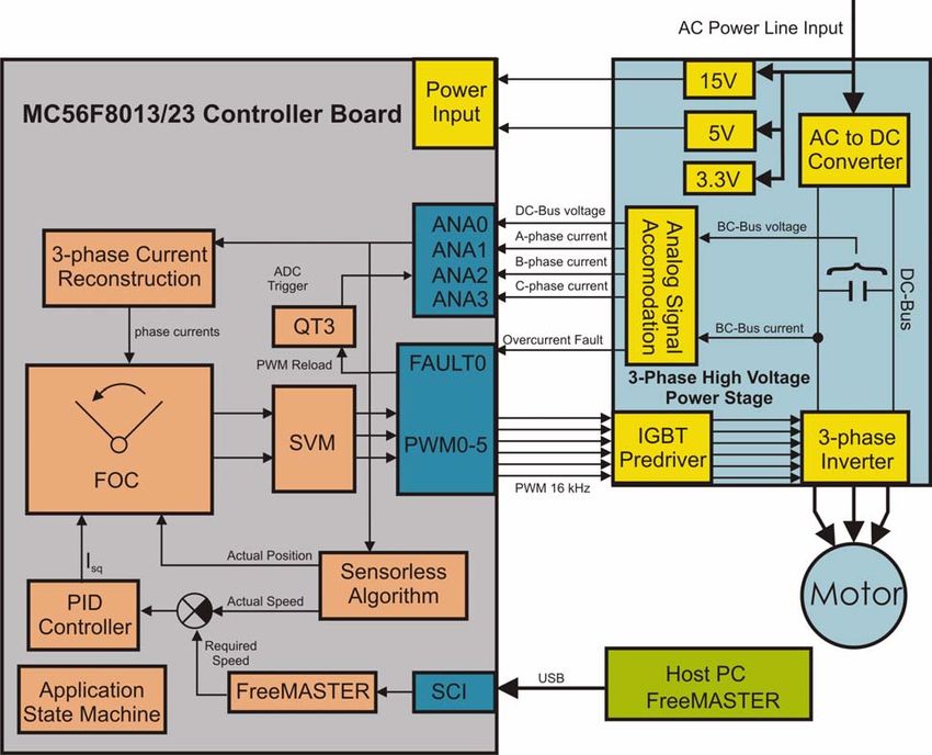
Sensorless PMSM Control for an H-axis Washing Machine Drive, Rev. 0

2                                                                     Freescale Semiconductor
Chapter 1
Introduction
Chapter 2
Washing Machine
2.1 Variable Speed Motor Drives . . . . . . . . . . . . . . . . . . . . . . . . . . . . . . . . . . . . . . . . . . . . . . .6
2.1.1 ACIM Speed Drive Control . . . . . . . . . . . . . . . . . . . . . . . . . . . . . . . . . . . . . . . . . .6
2.1.2 Permanent Magnet Motor . . . . . . . . . . . . . . . . . . . . . . . . . . . . . . . . . . . . . . . . . . .7
Chapter 3
Three-phase Permanent Magnet Synchronous Motors
3.1 Mathematical Model of a PM Synchronous Motor . . . . . . . . . . . . . . . . . . . . . . . . . . . . . . 10
3.1.1 Vector Transformations . . . . . . . . . . . . . . . . . . . . . . . . . . . . . . . . . . . . . . . . . . . . 11
3.1.2 PM Motor in the Stationary Reference Frame . . . . . . . . . . . . . . . . . . . . . . . . . . 13
3.1.3 PM Synchronous Motor in Rotating Reference Frame . . . . . . . . . . . . . . . . . . . . 15
3.2 Vector Control of PM Synchronous Motor . . . . . . . . . . . . . . . . . . . . . . . . . . . . . . . . . . . . 15
3.2.1 Fundamental Principle of Vector Control . . . . . . . . . . . . . . . . . . . . . . . . . . . . . . 15
3.2.2 Description of the Vector Control Algorithm . . . . . . . . . . . . . . . . . . . . . . . . . . . . 16
3.2.3 Current Control . . . . . . . . . . . . . . . . . . . . . . . . . . . . . . . . . . . . . . . . . . . . . . . . . . 18
3.2.4 Speed Control . . . . . . . . . . . . . . . . . . . . . . . . . . . . . . . . . . . . . . . . . . . . . . . . . . . 19
3.2.5 Flux Weakening Control . . . . . . . . . . . . . . . . . . . . . . . . . . . . . . . . . . . . . . . . . . . 20
3.2.6 Digital Controller . . . . . . . . . . . . . . . . . . . . . . . . . . . . . . . . . . . . . . . . . . . . . . . . .20
3.2.7 Space Vector Modulation (SVM) . . . . . . . . . . . . . . . . . . . . . . . . . . . . . . . . . . . . . 24
3.3 Position Sensorless Elimination . . . . . . . . . . . . . . . . . . . . . . . . . . . . . . . . . . . . . . . . . . . . 27
3.3.1 Rotor Alignment . . . . . . . . . . . . . . . . . . . . . . . . . . . . . . . . . . . . . . . . . . . . . . . . . 28
3.3.2 Open Loop Startup . . . . . . . . . . . . . . . . . . . . . . . . . . . . . . . . . . . . . . . . . . . . . . . 28
3.3.3 Back-EMF Observer . . . . . . . . . . . . . . . . . . . . . . . . . . . . . . . . . . . . . . . . . . . . . . 30
3.3.4 Speed and Position Extraction from the Estimated EEMF . . . . . . . . . . . . . . . . . 31
Chapter 4
System Concept
4.1 System Specifications . . . . . . . . . . . . . . . . . . . . . . . . . . . . . . . . . . . . . . . . . . . . . . . . . . . 35
4.2 Application Description . . . . . . . . . . . . . . . . . . . . . . . . . . . . . . . . . . . . . . . . . . . . . . . . . . 36
4.3 Control Process . . . . . . . . . . . . . . . . . . . . . . . . . . . . . . . . . . . . . . . . . . . . . . . . . . . . . . . .37
Chapter 5
Hardware
5.1 Hardware Implementation . . . . . . . . . . . . . . . . . . . . . . . . . . . . . . . . . . . . . . . . . . . . . . . . 39
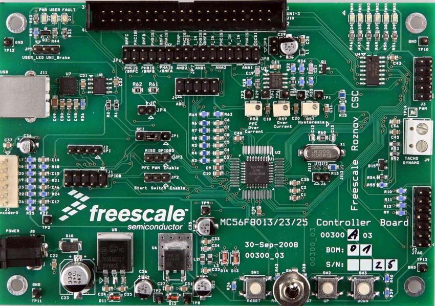
5.2 MC56F8013/23/25 Controller Board . . . . . . . . . . . . . . . . . . . . . . . . . . . . . . . . . . . . . . . . 40
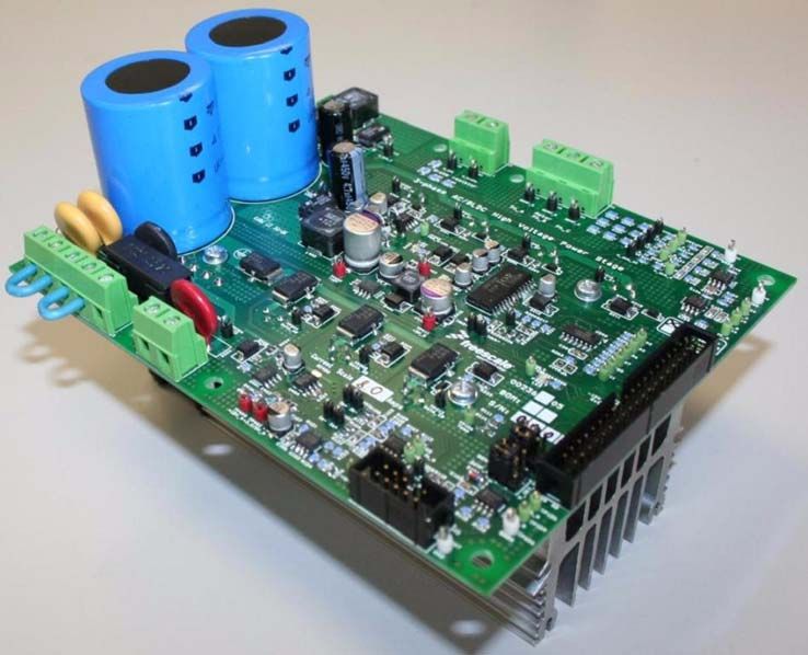
5.3 Three-Phase AC/BLDC High-Voltage Power Stage . . . . . . . . . . . . . . . . . . . . . . . . . . . . . 42
5.4 Motor Specifications — Example . . . . . . . . . . . . . . . . . . . . . . . . . . . . . . . . . . . . . . . . . . . 45
Sensorless PMSM Control for an H-axis Washing Machine Designer Reference Manual, Rev. 0
Freescale Semiconductor 1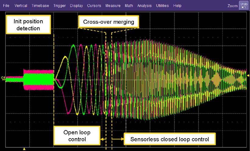
Chapter 6
Software Design
6.1 Introduction . . . . . . . . . . . . . . . . . . . . . . . . . . . . . . . . . . . . . . . . . . . . . . . . . . . . . . . . . . .47
6.2 Scaling Application Variables . . . . . . . . . . . . . . . . . . . . . . . . . . . . . . . . . . . . . . . . . . . . . . 47
6.2.1 Fractional Numbers Representation . . . . . . . . . . . . . . . . . . . . . . . . . . . . . . . . . . 47
6.2.2 Scaling Analog Quantities . . . . . . . . . . . . . . . . . . . . . . . . . . . . . . . . . . . . . . . . . .47
6.2.3 Scaling Angles . . . . . . . . . . . . . . . . . . . . . . . . . . . . . . . . . . . . . . . . . . . . . . . . . . 48
6.2.4 Scaling Parameters . . . . . . . . . . . . . . . . . . . . . . . . . . . . . . . . . . . . . . . . . . . . . . . 48
6.3 Software Flowchart . . . . . . . . . . . . . . . . . . . . . . . . . . . . . . . . . . . . . . . . . . . . . . . . . . . . . 50
6.4 Application Software States . . . . . . . . . . . . . . . . . . . . . . . . . . . . . . . . . . . . . . . . . . . . . . . 52
6.5 Feedback Measurement . . . . . . . . . . . . . . . . . . . . . . . . . . . . . . . . . . . . . . . . . . . . . . . . . 54
6.6 Application State Machine . . . . . . . . . . . . . . . . . . . . . . . . . . . . . . . . . . . . . . . . . . . . . . . . 58
6.7 Task Dispatching . . . . . . . . . . . . . . . . . . . . . . . . . . . . . . . . . . . . . . . . . . . . . . . . . . . . . . . 58
6.7.1 Task FAULT . . . . . . . . . . . . . . . . . . . . . . . . . . . . . . . . . . . . . . . . . . . . . . . . . . . . . 59
6.7.2 Task INIT . . . . . . . . . . . . . . . . . . . . . . . . . . . . . . . . . . . . . . . . . . . . . . . . . . . . . . . 59
6.7.3 Task CALIB . . . . . . . . . . . . . . . . . . . . . . . . . . . . . . . . . . . . . . . . . . . . . . . . . . . . . 60
6.7.4 Task ALIGN . . . . . . . . . . . . . . . . . . . . . . . . . . . . . . . . . . . . . . . . . . . . . . . . . . . . . 60
6.7.5 Task EXECUTE . . . . . . . . . . . . . . . . . . . . . . . . . . . . . . . . . . . . . . . . . . . . . . . . . 61
6.8 FreeMASTER Software . . . . . . . . . . . . . . . . . . . . . . . . . . . . . . . . . . . . . . . . . . . . . . . . . . 62
6.8.1 FreeMASTER Serial Communication Driver . . . . . . . . . . . . . . . . . . . . . . . . . . . .62
6.8.2 FreeMASTER Recorder . . . . . . . . . . . . . . . . . . . . . . . . . . . . . . . . . . . . . . . . . . . 64
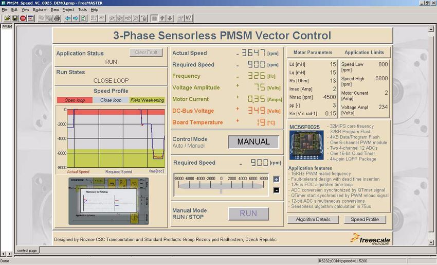
6.8.3 FreeMASTER Control Page . . . . . . . . . . . . . . . . . . . . . . . . . . . . . . . . . . . . . . . . 64
Chapter 7
Application Setup
7.1 MC56F8013/23/25 Controller Board Setup . . . . . . . . . . . . . . . . . . . . . . . . . . . . . . . . . . .68
7.2 Demo Hardware Setup . . . . . . . . . . . . . . . . . . . . . . . . . . . . . . . . . . . . . . . . . . . . . . . . . . 69
Chapter 8
Results and Measurements
8.1 System and Measurement Conditions . . . . . . . . . . . . . . . . . . . . . . . . . . . . . . . . . . . . . . . 73
8.1.1 Hardware Setup . . . . . . . . . . . . . . . . . . . . . . . . . . . . . . . . . . . . . . . . . . . . . . . . . 73
8.1.2 Start-up Performance . . . . . . . . . . . . . . . . . . . . . . . . . . . . . . . . . . . . . . . . . . . . . 73
8.1.3 Wash Cycle Performance . . . . . . . . . . . . . . . . . . . . . . . . . . . . . . . . . . . . . . . . . .75
8.1.4 Spin Cycle Performance . . . . . . . . . . . . . . . . . . . . . . . . . . . . . . . . . . . . . . . . . . . 77
8.2 Conclusion . . . . . . . . . . . . . . . . . . . . . . . . . . . . . . . . . . . . . . . . . . . . . . . . . . . . . . . . . . . . 77
Sensorless PMSM Control for an H-axis Washing Machine Designer Reference Manual, Rev. 0
2 Freescale Semiconductor
Chapter 1
Introduction
Recent world-wide interest towards environmental friendliness, water consumption, and energy saving
particularly impinge on the home appliance areas. Employing variable speed motor drives with PMSM
yield an opportunity to increase overall energy efficiency. Power density and intelligent control
consequently outperforms conventional uncontrolled drives. In PMSM achieving the variable speed drive
requires optimal motor speed determination and position by using a shaft position sensor to successfully
perform the PM motor field oriented control (FOC). Therefore, the aim is not to use this mechanical sensor
to measure the position directly, but employ some indirect technique to estimate the rotor position.
The variable speed motor drives are used in modern belt-driven washing machines, where the driving
motor works at lower speeds and higher torque levels during a tumble-wash cycle and high speed during
a spin-dry cycle. The proposed position estimation techniques are well suited for such applications
enabling better washing performance. An electronically controlled three phase interior PM motor provides
a unique feature set with higher efficiency and power density. A variable speed operation with optimum
performance of the interior PM motor can only be achieved when its excitation is precisely synchronized
with the instantaneous rotor position.
To be able to use FOC, the position of the rotor flux has to be known prior to any control action executed.
Therefore, a detection algorithm based on the injection of the pulsating HF signal in synchronous frame is
used to estimate the rotor position of the rotor at start-up. This technique avoids generating unwanted rotor
movements, common when conventional alignment processes are used. The enhanced back-EMF observer
detects the voltages induced by the stator windings PM flux. These signals are used to calculate the rotor
position and speed needed for control. Because the observed variables are not available at a low angular
speed, an open loop starting procedure is implemented. To test the performance both in steady-state and
transient operations, the resulting control structure has been fully analyzed through experiments.
The application software was implemented on a 16-bit fixed point DSC56F8023 digital signal controller.
Sensorless drive performance over a wide range of operating conditions within a washing machine is
demonstrated. It is also illustrated that the 16-bit digital signal controller that combines both MCU and
DSP capabilities can realize such a demanding control technique.

                      Sensorless PMSM Control for an H-axis Washing Machine Drive, Rev. 0
Freescale Semiconductor                                                                                   1-3
Introduction

               Sensorless PMSM Control for an H-axis Washing Machine Drive, Rev. 0
1-4                                                                              Freescale Semiconductor
Chapter 2
Washing Machine
The vertical axis (V-axis) washing machine dominates the non-European market today as residential
clothes washers. There is also a large portion of them in the commercial sector. In V-axis washers, clothes
move around a central agitator and must be fully immersed in water to be washed properly. The direct drive
V-axis washing machine used for development of the proposed sensorless algorithm is depicted in
Figure 2-1.
In horizontal axis (H-axis) washing machines, the wash drum rotates in alternate directions around a
horizontal axis instead of being fully immersed. The use of H-axis washing machines is expected to reduce
energy consumption significantly by reducing the water used and its heating. Currently, this type of
washing machine dominates the European market. Nowadays, a belted motor drive is conventionally used
in either type of washing machine. An ongoing effort is to replace such an approach using a direct drive
arrangement. This arrangement provides a significant improvement in reliability and reparability. Here,
the drive belt is eliminated and the direct drive washing machine’s cabinet consumes less space than its
belted counterpart.
The motor drive in the washing machine handles a wide range of speed. Torque and speed characteristics
of a washing machine drive is shown on Figure 2-1.

          Figure 2-1. Torque and speed characteristic of an electric drive for a washing machine

Figure 2-1 shows the drive operation in one direction, but the actual drive implementation has to be able
to perform speed reversal with the same torque and speed characteristic.
The actual time diagram of the tumble wash operation is shown in Figure 2-2. Here, the washtub operates
in slow speed. This figure shows a speed profile diagram where initially the washtub starts accelerating to
a low speed level, then there is a certain time interval of a steady spin, this is followed by the deceleration
back to zero speed, and then the washtub stops. This operation sequence is marked as positive in
Figure 2-2. After completion of this positive operation sequence the negative sequence is followed
employing the same speed profile, but targeting the negative speed level. These operations alternate during

                      Sensorless PMSM Control for an H-axis Washing Machine Drive, Rev. 0
Freescale Semiconductor                                                                                     2-5
Washing Machine

the tumble-wash cycle. The wash program chosen determines the overall time period of the wash cycle.
After completion of the wash cycle, the washing machine starts operation in the spin-dry cycle as shown
in Figure 2-2. The washing machine's washtub accelerates to a pre-defined high speed level for a spin-dry
cycle where it remains for a short time. Next, the washtub is commanded to decelerate either to a stop or
to proceed to a low speed level. This cycle might be repeated several times, depending on the wash
program chosen.

                              Figure 2-2. Washing machine operating cycles

Employing variable speed motor drives yields an opportunity to have more sophisticated washing
programs. This enables enhancing the appliance performance and increases overall energy efficiency. An
improved tumble-wash cycle can be achieved using various speed profiles with different speed ramps and
speed levels. The speed levels for the spin-dry cycle can also be set arbitrarily.
Thus washing machines equipped with variable speed drive and intelligent control consequently
outperform conventional and two speed washers.

2.1       Variable Speed Motor Drives
Variable speed drives (VSD) allow motors to operate continuously over a full range of speed. There are
different motor categories potentially applicable to drive washing machines such as an AC induction
machine (ACIM), PM motor, or a switched reluctance motor (SRM). The VSD overall efficiency is a by
product of the electronic drive efficiency and the motor efficiency.

2.1.1       ACIM Speed Drive Control
In general, to achieve a variable speed operation of the ACIM, the variable frequency and variable voltage
need to be supplied to the ACIM. This mode of operation is referred to as constant volt per Hz control. The
ACIM speed drive efficiency can be further improved by using FOC. This requires accurate velocity
information sensed by a speed or position sensor attached to the rotor. However, an additional extra sensor,
connector, and wirings increase the cost of the motor drives.

                     Sensorless PMSM Control for an H-axis Washing Machine Drive, Rev. 0
2-6                                                                                    Freescale Semiconductor
Washing Machine
2.1.2 Permanent Magnet Motor
Permanent magnet (PM) motors make use of permanent magnets to establish the flux instead of creating
it from the stator winding. Replacing the electromagnetic excitation by permanent magnets has several
advantages. The most obvious one is the absence of excitation losses in PM motors.
The need to use a shaft position sensor to successfully perform the control of the PM motor makes for
lowering the robustness and reliability of the overall system. Therefore, the aim is not to use this
mechanical sensor to measure the position directly but instead to employ some indirect techniques to
estimate the rotor position. These estimation techniques differ greatly in approach for estimating the
position or the type of motor they can be applied to.
Although there are several types of PM motors, they are broadly divided into brushless DC and AC
synchronous motors. According to the placements of the PM in the rotor PM motors it can be further
divided into several subgroups, each representing unique electrical characteristics. These include a
variation in the stator core saturation, stator resistance, or inductance variation and so on, and everything
dependent on the rotor position.
Sensorless PMSM Control for an H-axis Washing Machine Drive, Rev. 0
Freescale Semiconductor 2-7Washing Machine
Sensorless PMSM Control for an H-axis Washing Machine Drive, Rev. 0
2-8 Freescale SemiconductorChapter 3
Three-phase Permanent Magnet Synchronous Motors
Because the development of magnet materials, permanent magnet motors have become an attractive
solution compared to DC or induction motors for various drive applications. This permanent magnet (PM)
machine type offers important advantages. The moment of inertia can be kept minimal. The rotor
construction is more robust than DC motors. An alternative construction with buried (interior) magnets are
possible. Their efficiency is relatively high due to small rotor losses. For a short time, the motor currents
can be applied over the rated values. Due to the permanent magnetization, the motor can be operated
without a reactive current component which causes optimal inverter use.
There are two principal classes of permanent magnet AC machines. The first type, the permanent magnet
synchronous motor (PMSM) is sinusoidally excited. The second type, the trapezoidal excited machine is
the brushless DC (BLDC) motor. The construction differences are that while the stator windings of the
trapezoidal PM machines are concentrated into a narrow-phase pole, the windings of a sinusoidal machine
are typically distributed over multiple slots to approximate a sinusoidal distribution. These differences in
construction are reflected in their corresponding motion characteristics. This implies the consequence that
the first type of PMSM provides sinusoidal back-electromotive force (back-EMF) generation, and the
second type provides trapezoidal back-EMF.
The PM synchronous motor is a rotating electric machine with a classic three-phase stator like that of an
induction motor. The rotor has surface-mounted permanent magnets (see Figure 3-1).
Stator
Stator winding
(in slots)
Shaft
Rotor
Air gap
Permanent magnets
Figure 3-1. PM synchronous motor — cross section
The PM synchronous motor is equivalent to an induction motor. The air gap magnetic field is produced by
a permanent magnet, so that the rotor magnetic field is constant. The PM synchronous motors offer a
number of advantages when used in modern motion control systems. The use of a permanent magnet to
generate a substantial air gap magnetic flux makes it possible to design highly efficient PM motors.
Sensorless PMSM Control for an H-axis Washing Machine Drive, Rev. 0
Freescale Semiconductor 3-9Three-phase Permanent Magnet Synchronous Motors
The torque ripple associated with the sinusoidal PM (PMSM) machine is generally less than that
developed in trapezoidal (BLDC) machines. This provides the reasons that sinusoidal motors are
becoming popular in many different motor control applications such as washing machines, electrical
power steering, and electromechanical braking. This work targets the PMSM with only interior permanent
magnets.
3.1 Mathematical Model of a PM Synchronous Motor
A clear and comprehensive description of the synchronous machines dynamic behavior is a fundamental
requirement for their application in speed or torque controlled drive systems. The set of motor differential
equations (Equation 3-1) are well known books documented in numerous publications by reputed authors.
The stator voltage equations can be expressed as follows:
ua ia Ψa
d Eqn. 3-1
ub = RS ⋅ ib + Ψb
dt
uc ic Ψc
Equation 3-2 is the flux-linkage of each of the stator windings. and the equation for magnetic flux at the
rotor are:
cos ( θ e )
ψa L aa L ab L ca ia
⎛ 2 ⎞
ψ b = L L L ⋅ i b + ψ PM ⋅ cos ⎝ θ e – --3- π⎠
ab bb bc
Eqn. 3-2
ψc L ac L bc L cc ic
cos ⎛ θ e + --- π⎞
2
⎝ 3 ⎠
The PM synchronous machine is usually a symmetrical machine. All phase resistances, phase and mutual
inductances, and flux-linkages can be thought as equal or as a function of the rotor electrical position θ r
with a 120° displacement. In the case of an interior permanent magnet machine, the saliency is presented
in the motor and can be found as self and mutual inductances with variance in rotor position.
After applying substitutions to the stator phase equations (Equation 3-1), they can be transformed into the
following matrix form:
ua ia L aa L ab L ca ia L aa L ab L ca ia u backEMFa
u b = R S ⋅ i b + L ab L bb L bc d i ∂ dθ r
⋅ + L L L ⋅ -------
- ⋅ i + u backEMFb Eqn. 3-3
dt b ∂ t ab bb bc dt b
uc ic L ac L bc L cc ic L ac L bc L cc i c u backEMFc
Where the u backEMF vector column matrix means:
cos ( θ r )
u backEMFa
d cos ⎛ θ r – --- π⎞
2
u backEMFb = ω r ⋅ ψ PM ⋅ ⎝ 3 ⎠ Eqn. 3-4
dt
u backEMFc
cos ⎛ θ r + --- π⎞
2
⎝ 3 ⎠
The number of equations can be reduced if an appropriate transformation is introduced. They can be
transformed either into a stationary reference frame (a two phase system is fixed to the stator and is called
αβ) or a rotating reference frame (a two phase system is fixed to the rotor and is called dq).
Sensorless PMSM Control for an H-axis Washing Machine Drive, Rev. 0
3-10 Freescale SemiconductorThree-phase Permanent Magnet Synchronous Motors
Analogous to standard DC machines, and AC machines develop maximal torque when the armature
current is perpendicular to the flux linkage. Thus, if only the fundamental harmonic is considered, the
torque Te developed by an AC machine is given by:
pp i a ⋅ u backEMFa i b ⋅ u backEMFb i c ⋅ u backEMFc⎞ i a ⋅ u backEMFa i b ⋅ u backEMFb i c ⋅ u backEMFc
T e = ------ ⋅ ⎛ -------------------------------
- + -------------------------------- + -------------------------------- = -------------------------------
- + -------------------------------- + -------------------------------- Eqn. 3-5
2 ⎝ ωm ωm ωm ⎠ ωr ωr ωr
Where:
• ωm is the mechanical shaft speed of the rotor
• ωr is the electrical speed of the rotor in electrical radians per second
• pp is the number of poles for the motor.
Any mismatch between the back-EMF waveform and the corresponding phase currents result in a torque
ripple. The torque ripple is minimized by maintaining sinusoidal phase motor currents. Generally, it is
assumed that stator windings are approximated as sinusoidally distributed windings. The majority of the
PM synchronous motors are designed so that the stator windings produce a relatively fine approximation
of a sinusoidal distributed air gap magneto-motive force.
The relation between mechanical and electrical quantities are described by the mechanical equation as
follows:
d
J m ⋅ ----- ω r = T e – sign ( ω r ) ⋅ T L – B m ⋅ ω r – T f Eqn. 3-6
dt
Where:
• J m is a total mechanical inertia [ kg ⋅ m 2 ]
• B m viscous friction coefficient [ N ⋅ m ⋅ s ]
• T f is a Coulomb friction torque [ N ⋅ m ]
• T l is the mechanical load on the shaft [ N ⋅ m ]
3.1.1 Vector Transformations
This section gives an overview to the theory of the most commonly used reference frames and provides
equations that allow for easy conversion amongst them. Using these techniques, it is possible to transform
the phase variable machine description to another reference frame. The choice of the reference frame can
considerably simplify the complexity of the mathematical model of the PM synchronous motor.
Three-phase PM machines can be conventionally modeled using a phase variable notation as can bee seen
in Equation 3-3. However, for a three phase star-connected machine, the phase quantities are not
independent variables. Due to this redundancy, it is possible to transform the three phase system to an
equivalent two-phase representation. Hence, the transformation from three-phase to two-phase quantities
is as follows:
1 cos ⎛ --- π⎞ cos ⎛ --- π⎞
2 4 fa
fα 2 ⎝3 ⎠ ⎝3 ⎠
= --- ⋅ ⋅ fb Eqn. 3-7
fβ 3
0 sin ⎛ --- π⎞ sin ⎛ --- π⎞
2 2
fc
⎝3 ⎠ ⎝3 ⎠
Sensorless PMSM Control for an H-axis Washing Machine Drive, Rev. 0
Freescale Semiconductor 3-11Three-phase Permanent Magnet Synchronous Motors
This transformation in Equation 3-7 is valid for the current, voltage, and flux linkages as well. Introduced
transformation can be written in the inverse form as follows:
1 0
fa
cos ⎛ --- π⎞ sin ⎛ --- π⎞
2 2 fα
fb = ⎝3 ⎠ ⎝3 ⎠ ⋅ Eqn. 3-8
fβ
fc
cos ⎛ --- π⎞ sin ⎛ --- π⎞
4 4
⎝3 ⎠ ⎝3 ⎠
Transformation Equation 3-7 and Equation 3-8 are commonly known as the forward Clarke and the
inverse Clarke transformation, respectively. Defined vector quantities are shown in Figure 3-2.
Figure 3-2. Stationary reference frame in relation with phase quantities
The real α – axis of the defined stationary coordinate system is chosen to coincide with the a – axis . The
β – axis lies in quadrature with the α – axis . This reference frame with α, β quantities is known as a
stationary reference frame that is fixed to the stator.
Meanwhile the vectors of the current, voltage and flux linkages rotate around these axes at a rate equal to
the angular frequencies of the corresponding phase quantities. Besides this stationary reference frame
attached to the stator, there can be formulated a general reference frame that rotates vector quantities
through a known angle. This can be represented by following matrix formula as:
fd
= cos ( θ ) sin ( θ ) ⋅ i α
fq – sin ( θ ) cos ( θ ) iβ Eqn. 3-9
The motor current vector consists of the direct axis component id and the component iq, that is called the
quadrature axis component. The relationship of the direct and quadrature components of the current vector
in the original stationary two-axis reference frame and the rotating reference frame is shown in Figure 3-3.
Sensorless PMSM Control for an H-axis Washing Machine Drive, Rev. 0
3-12 Freescale SemiconductorThree-phase Permanent Magnet Synchronous Motors
Figure 3-3. Rotating reference frame in relation with stationary reference frame
This transformation is known as the inverse Park transformation. The transformation from a rotating to a
stationary reference frame is given as:
fα cos ( θ ) – sin ( θ ) ⋅ f d
=
fβ sin ( θ ) cos ( θ ) fq
Eqn. 3-10
This vector transformation from rotating reference frame to the stationary one is commonly known as the
forward Park transformation. The elimination of position dependency from the PM motor electrical
variables are the main advantage of an introduced vector rotation, see Equation 3-9 and Equation 3-10.
3.1.2 PM Motor in the Stationary Reference Frame
The PM motor equation in the stationary reference frame ( αβ coordinates) can be expressed in the scalar
forms of the stator voltage and flux linkage defined as:
uα RS 0 iα d ψα
= ⋅ + 1 0 ⋅
uβ 0 RS iβ 0 1 d t ψβ
Eqn. 3-11
This is an equivalent to Equation 3-12. There can be defined two useful terms by establishing direct axis
inductance L d , and quadrature axis inductance L q . The mean inductance L 0 and differential inductance ΔL
are as follows:
Ld + Lq
L 0 = -----------------
-
2
Ld – Lq Eqn. 3-12
ΔL = ------------------
2
Where L 0 is the average inductance, ΔL is the zero-to-peak differential inductance is a direct measure of
the spatial modulation of the inductance. In a surface mounted machine L q and L d are almost equal, so ΔL
is very small. The buried magnet machine has a large difference between the d-axis and q-axis inductance
due to the spatial modulation produced by the difference in the flux coupling between the stator and rotor.
The corresponding flux-linkage equations are:
Sensorless PMSM Control for an H-axis Washing Machine Drive, Rev. 0
Freescale Semiconductor 3-13Three-phase Permanent Magnet Synchronous Motors
ψα L 0 + ΔL ⋅ cos ( 2θ r ) ΔL ⋅ sin ( 2θ r ) iα cos ( θ r )
= ⋅ + ψ PM ⋅
ψβ ΔL ⋅ sin ( 2θ r ) L 0 – ΔL ⋅ cos ( 2θ r ) iβ sin ( θ r ) Eqn. 3-13
After substitution, equation Equation 3-13 is derived when Equation 3-12 and Equation 3-13 are
combined in such way that Equation 3-12 flux linkages are replaced with Equation 3-13. The equation
described is:
uα iα L 0 + ΔL ⋅ cos ( 2θ r ) ΔL ⋅ sin ( 2θ r ) d iα
= RS ⋅ + ⋅
uβ iβ ΔL ⋅ sin ( 2θ r ) L 0 – ΔL ⋅ cos ( 2θ r ) dt i
β
Eqn. 3-14
⎛ – sin ( 2θ r ) cos ( 2θ r ) cos ( θ r ) ⎞
ω r ⋅ ⎜ 2 ΔL + ψ PM ⋅ ⎟
⎝ cos ( 2θ r ) sin ( 2θ r ) sin ( θ r ) ⎠
Here, the inductance matrix is represented by a PM motor in a rotating reference frame as:
L 0 + ΔL ⋅ cos ( 2θ r ) ΔL ⋅ sin ( 2θ r )
L ( 2θ r ) =
ΔL ⋅ sin ( 2θ r ) L 0 – ΔL ⋅ cos ( 2θ r ) Eqn. 3-15
Electromagnetic torque can be expressed in terms of the stator flux and stator current as below:
3
T e = --- ⋅ pp ⋅ ( ψ α ⋅ i β – ψ β ⋅ i α )
2 Eqn. 3-16
The electromagnetic torque T e developed by PM synchronous motors can be divided into two
components. The first component is created by contribution of the permanent magnet flux ψ PM and is
called synchronous torque. The second component referred to as reluctance torque arises due to rotor
saliency where the rotor tends to align with the minimum reluctance. So the resulting torque is given by:
T e = T syn + T rel
Eqn. 3-17
Where, for the stationary reference frame, synchronous and reluctance torque components are described
as follows:
3
T syn = --- ⋅ pp ⋅ ψ PM ⋅ ( i β cos ( θ β ) + i α sin ( θ r ) )
2 Eqn. 3-18
T rel = --- ⋅ pp ⋅ ⎛ – ΔLi α i β cos ( 2θ r ) – --- ( i α2 + i β2 ) sin ( 2θ r )⎞
3 1
2 ⎝ 2 ⎠
Eqn. 3-19
Although a quadrature axis PMSM model in a stationary reference frame is already simple, when
compared to the full three phase model. It still contains a position variant inductance matrix. Both currents
and voltages are also AC values that make it difficult for a control structure. Therefore an additional
quadrature model is introduced.
Sensorless PMSM Control for an H-axis Washing Machine Drive, Rev. 0
3-14 Freescale SemiconductorThree-phase Permanent Magnet Synchronous Motors
3.1.3 PM Synchronous Motor in Rotating Reference Frame
The vector transformations of Equation 3-7 and Equation 3-9 are used to derive this model, assuming that
the transformation argument θ is equal to the electrical rotor position θ r . The stator voltage equation in the
rotating reference frame fixed to the rotor is given as:
ud RS 0 id s ωr ψd
= ⋅ + ⋅ Eqn. 3-20
uq 0 RS iq –ωr s ψq
Where p represents a derivative operator. The stator flux linkage is expressed as:
ψd Ld 0 id
= ⋅ + ψ PM ⋅ 1
ψq 0 Lq iq 0
Eqn. 3-21
In a salient PM synchronous machine, there is a difference between the rotor d-axis (main flux direction)
and the rotor q-axis (main torque producing direction) inductances L d ≠ L q . After substitution, the flux
linkage equation into the stator voltage equation, then the interior permanent magnet motor expressed in
the stationary reference frame can be derived forming the following equation.
ud RS –ωe Lq id Ld 0 d id
= ⋅ + ⋅ + ω e ψ PM ⋅ 0
uq ωe Ld RS iq 0 Lq d t iq 1
Eqn. 3-22
Electromagnetic torque can be expressed in terms of the stator flux and stator current as below:
3
T e = --- ⋅ pp ⋅ ( ψ d ⋅ i q – ψ q ⋅ i d ) Eqn. 3-23
2
Electromagnetic torque T e developed by PM synchronous motors can be divided into two components.
The first component is created by contribution of the permanent magnet flux ψ PM and is called
synchronous torque. The second component, referred to as reluctance torque, arises due to rotor saliency,
where the rotor tends to align with minimum reluctance. So the resulting torque is given by:
T e = T syn + T rel Eqn. 3-24
Where, for the stationary reference frame, synchronous and reluctance torque components are described
as follows:
3
T syn = --- ⋅ pp ⋅ ψ PM ⋅ i q
2 Eqn. 3-25
3 Eqn. 3-26
T rel = --- ⋅ pp ⋅ ΔLi d i q
2
3.2 Vector Control of PM Synchronous Motor
3.2.1 Fundamental Principle of Vector Control
High-performance motor control is characterized by smooth rotation over the entire speed range of the
motor, full torque control at zero speed, and fast acceleration and deceleration. To achieve such control,
Sensorless PMSM Control for an H-axis Washing Machine Drive, Rev. 0
Freescale Semiconductor 3-15Three-phase Permanent Magnet Synchronous Motors
vector control techniques are used for PM synchronous motors. The vector control techniques are usually
also referred to as field-oriented control (FOC). The basic idea of the vector control algorithm is to
decompose a stator current into a magnetic field-generating part and a torque-generating part. Both
components can be controlled separately after decomposition. The structure of the motor controller is then
as simple for a separately excited DC motor.
Figure 3-4 shows the basic structure of the vector control algorithm for the PM synchronous motor. To
perform vector control it is necessary to perform these steps:
1. Measure the motor quantities (phase voltages and currents).
2. Transform them into the two-phase system (α,β) using a Clarke transformation.
3. Calculate the rotor flux space vector magnitude and position angle.
4. Transform stator currents into the d, q reference frame using a Park transformation.
Also keep these points in mind:
• The stator current torque (isq) and flux (isd) producing components are separately controlled.
• The output stator voltage space vector is calculated using the decoupling block.
• The stator voltage space vector is transformed by an inverse Park transformation back from the d,
q reference frame into the two-phase system fixed with the stator.
• The output three-phase voltage is generated using space vector modulation.
To be able to decompose currents into torque and flux producing components (isd, isq), the position of the
motor-magnetizing flux must be known. This requires accurate sensing of the rotor position and velocity.
Incremental encoders or resolvers attached to the rotor are naturally used as position transducers for vector
control drives.
In some applications, the use of speed and position sensors are not desirable. In these applications the aim
is not to measure the speed and position directly, but to instead employ some indirect techniques to
estimate the rotor position. Algorithms that do not employ speed sensors are called “sensorless control.”
Figure 3-4. Vector control transformations
3.2.2 Description of the Vector Control Algorithm
The overview block diagram of the implemented control algorithm is illustrated in Figure 3-5. Similar to
other vector-control-oriented techniques, it is possible to control the field and torque of the motor
separately. The aim of this control is to regulate the motor speed at a predefined level. The speed command
value is set by high level control. The algorithm is executed in two control loops. The fast inner control
Sensorless PMSM Control for an H-axis Washing Machine Drive, Rev. 0
3-16 Freescale SemiconductorThree-phase Permanent Magnet Synchronous Motors
loop is executed with a hundred μsec period range. The slow outer control loop is executed with a period
of msec range.
To achieve the goal of the PM synchronous motor control, the algorithm uses feedback signals. The
essential feedback signals are three-phase stator current and stator voltage. For the stator voltage, the
regulator output is used. For correct operation, the presented control structure requires a speed feedback
on the motor shaft. In the case of the presented algorithm, a sensorless algorithm is used.
The fast control loop executes two independent current control loops. They are the direct and
quadrature-axis current (isd,isq) PI controllers. The direct-axis current (isd) is used to control the rotor-
magnetizing flux. The quadrature-axis current (isq) corresponds to the motor torque. The current PI
controllers’ outputs are summed with the corresponding d and q axis components of the decoupling stator
voltage. Thus, the desired space vector for the stator voltage is obtained and then applied to the motor. The
fast control loop executes all the necessary tasks to be able to achieve an independent control of the stator
current components. These include:
• Three-phase current reconstruction
• Forward Clark transformation
• Forward and backward Park transformations
• Rotor magnetizing flux position evaluation
• DC-bus voltage ripple elimination
• Space vector modulation (SVM)
Figure 3-5. PMSM vector control algorithm overview
The slow control loop executes the speed controller and lower priority control tasks.The PI speed
controller output sets a reference for the torque producing quadrature axis component of the stator current
i q_ref and flux producing current i d_ref .
Sensorless PMSM Control for an H-axis Washing Machine Drive, Rev. 0
Freescale Semiconductor 3-17Three-phase Permanent Magnet Synchronous Motors
3.2.3 Current Control
Figure 3-5 shows the structure d-q current control. It is the most inner loop in the vector control of PM
synchronous motor. In vector control techniques, both the cross-coupling terms as well as the back-EMF
induced voltage term in Equation 3-22 are compensated using a feed-forward voltage, as follows:
decoupling
ud = –ωr Lq iq
decoupling
uq = ω r L d i d + ω r ψ PM Eqn. 3-27
This helps to establish full decoupled d and q axis current loops, allows independent control of current d
and q components, and simplifies the motor circuit. The resultant dynamics are is:
Eqn. 3-28
di d
u d = Ri d + L d
dt
di q
u q = Ri q + L q
dt
Both channels employ a PI controller with additional decoupling terms that reduce dynamic interactions.
Both equations are structurally identical, therefore the same controller design approach can be applied for
both d and q controllers. In the case that inductance parameter Ld (Lq) are not equal, then this results with
the controllers having different Kp, Ki gains.To simplify the PI controllers design, the effects of AD and
inverter transportation delay are neglected.
Considering a general form of a closed-loop with the PI controller and RL model as a plant, the closed-loop
transfer function of the reference response is derived in a Laplace form, as follows:
Kp s + Ki K Eqn. 3-29
G C ( s ) = --------------------
- = K p + -----i
s s
Plant model is:
1
----
1 R
G P = ---------------- = ----------------
Ls + R L
---- s + 1 Eqn. 3-30
R
The characteristic polynomial of the transfer function G(s) form reveals in the closed-loop that it is a
second order system.
KP K
( )G ( )
------s + -----I
I(s) G s s L L
G ( s ) = --------- = --------------------------------------
C P
- = -------------------------------------------------
I(s) 1 + G C ( s )G P ( s ) K + R KI
s + ⎛ -----------------⎞ s + -----
2 P
⎝ L ⎠ L Eqn. 3-31
However, the PI controller introduces a zero to the closed-loop transfer function for commanded changes,
K
and it is located at – ------I . This derivative characteristic of the loop increases the system overshoot by
KP
lowering the potential closed-loop bandwidth. It might be compensated by introducing a zero cancellation
block in the feedforward path that has the following transfer function.
Sensorless PMSM Control for an H-axis Washing Machine Drive, Rev. 0
3-18 Freescale SemiconductorK Three-phase Permanent Magnet Synchronous Motors
------I
KP
G ZC ( s ) = --------------- Eqn. 3-32
K
s + ------I
KP
The resulting transfer function with an implemented zero cancellation is then:
K KP K
------I ------s + -----I
KP L L
G ( s ) = --------------- ⋅ ------------------------------------------------- Eqn. 3-33
K I 2 ⎛ K P + R⎞ K
s + ------ s + ----------------- s + -----I
KP ⎝ L ⎠ L
TheKI
zero cancellation transfer function Gzc(s) has to be designed to compensate the closed-loop zero at
– ------ , but with the unity DC gain. The unity DC gain ensures the closed-loop gain to be the same with or
KP
without zero cancellation, thus preserving the original loop gain. The DC gain can be verified by
calculating Equation 3-32 with s=0.
By having the closed-loop zero canceled, the PI controller can be designed by comparing the closed-loop
characteristic polynomial with that of a standard second order system as:
2
ω0
G W ( s ) = --------------------------------------
2
-
2
s + 2ξω 0 s + ω 0 Eqn. 3-34
Comparison can be made as follows:
K P + R⎞ K
s + ⎛ ----------------
2 2 2
- s + -----I = s + 2ξω 0 s + ω 0
⎝ L ⎠ L
Eqn. 3-35
Where ω0 is the natural frequency of the closed-loop system (loop bandwidth) and ξ is the loop
attenuation. The proportional and integral gains of the PI controller can be calculated from Equation 3-35
as:
K P = 2ξω 0 L – R
2
Eqn. 3-36
KI = ω0 L
Equation 3-36 describes a PI controller design in time domain. However, in the digital implementation, the
control loop is calculated in discrete steps rather than continuously, therefore a discrete representation of
the controller has to be used. Implementing the control system in a digital domain also inserts a
transportation delay into the control loop. This delay is associated with the hold where each value of u(kT)
is held until the next value is available.
3.2.4 Speed Control
The model of the plant in the speed loop is derived from the machine mechanical equation (2.8). Hence
the model transfer function is given as follows:
Where kT is the torque constant representing the ratio between torque and current, similar to the current
control loop, the speed loop is closed by a PI controller that enables the speed control with zero steady state
Sensorless PMSM Control for an H-axis Washing Machine Drive, Rev. 0
Freescale Semiconductor 3-19Three-phase Permanent Magnet Synchronous Motors
error. The speed controller directly drives the required current that is the input to the current loop and hence
the required torque when multiplied by kT. Because the mechanical time constants are bigger than the
electrical time constants, the speed loop is sampled slower than the current loop. The current loop
transients can be considered to be settled between the speed loop sampling instants that allow to substitute
the whole current loop by a first order lag. The difference in mechanical and electrical time constants also
implies that the speed controller will be saturated most of the time during the speed transient, this is
because the current limit is reached much faster than the speed settling time. Therefore, it is crucial for the
speed controller to have an anti-windup implemented.
In contrast to the current control loop, the parameters of the plant model in speed loop are usually difficult
to determine. This is predominantly caused by variations in the system lumped inertia that changes with
each mechanical arrangement of the system. The mechanical load on the motor shaft acts as a disturbance
to the speed control loop, making the loop characteristic non-linear. Therefore, the mathematical
derivation of the speed controller gains is difficult. However, it remains possible to determine the speed
loop bandwidth through experiments. One possible approach is to use a sinusoidal reference to drive the
commanded speed and observe the attenuation and phase shift of the measured speed.
3.2.5 Flux Weakening Control
The operation beyond the machine base speed requires the PWM inverter to provide output voltages higher
than its output capability limited by its dc-link voltage. This in turn saturates the motor drive control
system. By manipulating the -axis current into the machine it has the desired effect of weakening its field
and the need for higher voltages as the machine exceeds its base speed. An anti-saturation control loop is
then implemented in this software to regulate the duty-cycle to a desired maximum value under this
condition, using as control variable the d-axis current.
3.2.6 Digital Controller
The PI algorithm in the continuous time domain Equation 3-29 can be rewritten into the discrete time
domain by approximating the integral and derivative terms. The integral term is approximated with the
Backward Euler Method, also known as backward rectangular or right-hand approximation as follows:
u I ( k ) = u I ( k – 1 ) + ΔT s e ( k ) Eqn. 3-37
The discrete time domain representation of the PI algorithms:
u ( k ) = KP e ( k ) + uI ( k – 1 ) + KI e ( k ) Eqn. 3-38
Where:
• e(k)—Input error at step k; processed by the P and I terms
• u(k)—Controller output at step k
• Kp—Proportional gain
• Ki—Integral gain
• ΔT S —Sampling time (period) [sec]
The discrete time domain representation of the PI algorithm scaled into the fractional range.
Sensorless PMSM Control for an H-axis Washing Machine Drive, Rev. 0
3-20 Freescale SemiconductorThree-phase Permanent Magnet Synchronous Motors
FRAC FRAC FRAC
u FRAC ( k ) = K P e FRAC ( k ) + u I ( k – 1 ) + KI e FRAC ( k )
Eqn. 3-39
The PI algorithm in Equation 3-39 is implemented in the parallel (non-interacting) form allowing the user
to define the P and I parameters independently without interaction. The PI controller parameters in
fractional representation are determined as follows:
FRAC E MAX
KP = K P ---------------
U MAX
E MAX Eqn. 3-40
FRAC
KI = K I ΔT S --------------
-
U MAX
Where:
• Emax—Input error maximal range, usually controller error range is the same as the controlled
variable
• Umax—Controller output maximal range
The individual parameter (such as KIsc) of the PI algorithm is represented by two parameters in the
processor implementation:
FRAC i16PropGainShift
KP = f16PropGain ⋅ 2
FRAC i16IntegGainShift
KI = f16IntegGain ⋅ 2 Eqn. 3-41
To determine parameters for the GFLIB_ControllerPIp function, first the calculation of the appropriate
shift is derived as follows:
FRAC – i16PropGainShift
( 1 > KP ⋅2 ≥ 0.5 ) ⁄ ln
FRAC
( ln ( 1 ) > ln ( K P ) – i16PropGainShift ⋅ ln ( 2 ) ≥ ln ( 0.5 ) )
FRAC FRAC Eqn. 3-42
ln ( K P ) – ln ( 1 ) ln ( K P ) – ln ( 0.5 )
- < i16PropGainShift ≤ --------------------------------------------------
---------------------------------------------
ln ( 2 ) ln ( 2 )
ln ( 1 ) = 0
Due to simplification only the left side of Equation 3-42 is considered where ln(1) is omitted.
FRAC
ln ( K P )
-------------------------- < i16PropGainShift
ln ( 2 ) Eqn. 3-43
FRAC
log ( K P ) – log ( 0.5 )
i16PropGainShift = ceil ⎛ --------------------------------------------------------⎞
⎝ log ( 2 ) ⎠
Eqn. 3-44
FRAC – i16PropGainShift
f16PropGain = KP ⋅2
Sensorless PMSM Control for an H-axis Washing Machine Drive, Rev. 0
Freescale Semiconductor 3-21Three-phase Permanent Magnet Synchronous Motors
FRAC
log ( K I ) – log ( 0.5 )⎞
i16IntegGainShift = ceil ⎛ -------------------------------------------------------
-
⎝ log ( 2 ) ⎠
FRAC – i16IntegGainShift
f16IntegGainShift = K I ⋅2
Eqn. 3-45
Division is usually a real number. Therefore “ceiling” returns the number rounded up, away from zero, and
to the nearest multiple of significance.
In the case of the recurrent form of the Proportional-Integral (PI) controller, different techniques are used
to convert the continuous PI controller function into the discrete representation.
NOTE
The continuous function can only be approximated and the discrete representation can never be exactly
equivalent. The resulting difference equation derived by the discretization method is in the form as
reported below:
u ( k ) = u ( k – 1 ) + CC1 ⋅ e ( k ) + CC2 ⋅ e ( k – 1 )
Eqn. 3-46
The transition from the continuous to the discrete time domain reveals the following controller coefficients
Table 3-1. Controller coefficients
Controller Backward Forward
Bilinear transformation
Coefficients rectangular rectangular
CC1 K I ΔT S K P + K I ΔT S KP
K P + ---------------
-
2
CC2 K I ΔT S –KP – K P + K I ΔT S
– K P + ---------------
-
2
Where:
• KP —Proportional gain
• KI —Integral gain
• TS —Sampling period
The discrete time domain representation of the recurrent PI algorithm scaled into the fractional range is:
f16Uk = f32Acc + f16CC1 ⋅ f16Error + f16CC2 ⋅ f16ErrorK_1
Eqn. 3-47
Where f32Acc is the accumulated controller portion over time and is used as the internal variable of this
algorithm. The f16CC1 and f16CC2 are recurrent controller coefficients that are adapted as:
Sensorless PMSM Control for an H-axis Washing Machine Drive, Rev. 0
3-22 Freescale SemiconductorThree-phase Permanent Magnet Synchronous Motors
Error_max
f16CC1 = CC1 ⋅ --------------------------
U_max Eqn. 3-48
Error_max
f16CC2 = CC2 ⋅ --------------------------
U_max Eqn. 3-49
For proper operation of the recurrent PI controller implemented on the 16 and 32-bit DSC care must be
taken due to the fixed point representation of individual values. A scaling shift ui16NShift is introduced
to be scaled to the 16-bit fixed point format. Then, fractional representation on the DSC of the recurrent
PI controller is calculated by the following formula as:
f16Uk = f16Acc + f16CC1Sc ⋅ f16Error + f16CC2Sc ⋅ f16ErrorK1 Eqn. 3-50
Where:
– ui16NShift
f16CC1Sc = f16CC1 ⋅ 2
Eqn. 3-51
– ui16NShift
f16CC2Sc = f16CC2 ⋅ 2
Eqn. 3-52
ui16NShift is chosen so that the coefficients reside within the common range . In addition,
the ui16NShift is chosen as a power of 2. The final de-scaling is a simple shift operation.
log ( abs(f16CC1) ) log ( abs ( f16CC2 ) )
ui16NShift = max ⎛ ceil ⎛ --------------------------------------------⎞ , ceil ⎛ ----------------------------------------------⎞ ⎞
⎝ ⎝ log 2 ⎠ ⎝ log 2 ⎠⎠
Eqn. 3-53
The zero cancellation transfer function can also be transformed into Z-domain using the Backward Euler
Method as follows:
–1
1–z
s ≈ ----------------
ΔT S
1 z
--- = ----------- ⋅ ΔT S
s z–1
Eqn. 3-54
Sensorless PMSM Control for an H-axis Washing Machine Drive, Rev. 0
Freescale Semiconductor 3-23Three-phase Permanent Magnet Synchronous Motors
KI
a = ------
KP
aΔT S
----------------------
a aΔT 1 + a ΔT S
G ZC ( z ) = ------------------------
- = S
----------------------------------- = --------------------------------------
-
1–z
–1 –1
1 – z + aΔT S 1 –1 Eqn. 3-55
---------------- + a 1 – ----------------------z
ΔT S 1 + a ΔT S
KI
------ΔT
KP S
---------------------------
KI K I ΔT S
1 + ------ ΔT S -----------------------------
KP K P + K I ΔT S
G ZC ( z ) = -------------------------------------------
- = ---------------------------------------------
-
1 –1 KP –1
1– --------------------------
- z 1 – -----------------------------z
K K P + K I ΔT S
1 + ------I ΔT S
KP
The discrete implementation is therefore given by:
K I ΔT S KP
y ( k ) = ----------------------------- ⋅ x ( k ) + ----------------------------- ⋅ y(k – 1)
K P + K I ΔT S K P + K I ΔT S
Eqn. 3-56
It is clear that Equation 3-56 is a simplified form of the first order low-pass filter in IIR implementation.
The zero cancellation block physically behaves as a low pass filter, smoothing the input command.
The GDFLIB_FilterIIR1 function calculates the first order infinite impulse response (IIR) filter. The IIR
filters are also called recursive filters because both the input and the previously calculated output values
are used for calculation. The first order IIR filter in the Z-domain is given as:
–1
b1 + b2 z
H ( z ) = -----------------------
–1
-
1 + a2 z
Eqn. 3-57
Transformed into a time domain difference equation:
y ( k ) = b1 ⋅ x ( k ) + b2 ⋅ x ( k – 1 ) + a2 ⋅ y ( k – 1 ) Eqn. 3-58
This function is used to perform a zero cancellation transfer function with the following parameters:
K I ΔT S
b 1 = -----------------------------
K P + K I ΔT S
b2 = 0 Eqn. 3-59
KP
a 2 = -----------------------------
K P + K I ΔT S
3.2.7 Space Vector Modulation (SVM)
The space vector modulation (SVM) can directly transform the stator voltage vectors from the two-phase
α,β-coordinate system into the pulse-width modulation (PWM) signals (duty cycle values).
Sensorless PMSM Control for an H-axis Washing Machine Drive, Rev. 0
3-24 Freescale SemiconductorThree-phase Permanent Magnet Synchronous Motors
The standard technique of output voltage generation uses an inverse Clarke transformation to obtain
three-phase values. Using the phase voltage values, the duty cycles needed to control the power stage
switches are then calculated. Although this technique gives good results, space vector modulation is more
straightforward (valid only for transformation from the α,β-coordinate system).
The basic principle of the standard space vector modulation technique can be explained with the help of
the power stage schematic diagram given in Figure 3-6. Eight possible switching states (vectors) are
feasible regarding the three-phase power stage configuration. See Figure 3-6. These states are given by
combinations of the corresponding power switches. A graphical representation of all the combinations is
the hexagon shown in Figure 3-7. There are six non-zero vectors, U0, U60, U120, U180, U240, U300, and two
zero vectors, O000 and O111, defined in α,β coordinates.
Id0
+
uDC-Bus /2 = S At S Bt S Ct
-
+
uDC-Bus /2 IB
= S Ab IA S Bb S Cb IC
-
u AB u BC
u CA
B
uR
ub
uL
u ib
ua O u ic
u L u ia uL
uR uc
uR
A C
Figure 3-6. Power stage schematic diagram
The combination of ON/OFF states in the power stage switches for each voltage vector is coded by the
three-digit number in parentheses. See Figure 3-7. Each digit represents one phase. For each phase, a value
of one means that the upper switch is ON and the bottom switch is OFF. A value of zero means that the
upper switch is OFF and the bottom switch is ON. These states, together with the resulting instantaneous
output line-to-line voltages, phase voltages, and voltage vectors, are listed in Table 3-2.
Sensorless PMSM Control for an H-axis Washing Machine Drive, Rev. 0
Freescale Semiconductor 3-25Three-phase Permanent Magnet Synchronous Motors
Table 3-2. Switching patterns and resulting instantaneous
a b c Ua Ub Uc UAB UBC UCA Vector
0 0 0 0 0 0 0 0 0 O000
1 0 0 2UDC-Bus/3 –UDC-Bus/3 –UDC-Bus/3 UDC-Bus 0 –UDC-Bus U0
1 1 0 UDC-Bus/3 UDC-Bus/3 –2UDC-Bus/3 0 UDC-Bus –UDC-Bus U60
0 1 0 –UDC-Bus/3 2UDC-Bus/3 –UDC-Bus/3 –UDC-Bus UDC-Bus 0 U120
0 1 1 –2UDC-Bus/3 UDC-Bus/3 UDC-Bus/3 –UDC-Bus 0 UDC-Bus U240
0 0 1 –UDC-Bus/3 –UDC-Bus/3 2UDC-Bus/3 0 –UDC-Bus UDC-Bus U300
1 0 1 UDC-Bus/3 –2UDC-Bus/3 UDC-Bus/3 UDC-Bus –UDC-Bus 0 U360
1 1 1 0 0 0 0 0 0 O111
U120 U60
(010) β-axis (110)
[1/√3,-1] [1/√3,1]
Basic Space Vector II.
T60/T*U60 Maximal phase
voltage magnitude = 1
III.
US
U180 uβ U0
(011) (100) α-axis
[-2/√3,0] O000 O111 [2/√3,0]
(000) (111) uα
T0/T*U0
IV. 30 degrees VI.
Voltage vector components
in α, β axis
V.
[-1/√3,-1] [-1/√3,1]
U240 U300
(001) (101)
Figure 3-7. Basic space vectors and voltage vector projection
The SVM is a technique used as a direct bridge between the vector control (voltage space vector) and the
PWM.
The SVM technique consists of several steps:
1. Sector identification
2. Space voltage vector decomposition into directions of sector base vectors Ux, and Ux±60
3. PWM duty cycle calculation
The principle technique of the SVM is the application of the voltage vectors UXXX and OXXX and in
some instances the mean vector of the PWM period tPWM is equal to the desired voltage vector.
Sensorless PMSM Control for an H-axis Washing Machine Drive, Rev. 0
3-26 Freescale SemiconductorThree-phase Permanent Magnet Synchronous Motors
This method gives the greatest variability in arranging the zero and non-zero vectors during the PWM
period. You can arrange these vectors to lower switching losses, or to reach a different result such as
center-aligned PWM, edge-aligned PWM, minimal switching, and so on.
For the chosen SVM, this rule is defined:
• The desired space voltage vector is created only by applying the sector base vectors: the non-zero
vectors on the sector side (Ux, Ux±60), and the zero vectors (O000 or O111).
The following define the principle technique of the SVM:
t PWM × U S [ α, β ] = t 1 × U x + t 2 × ( U x ± 60 + t 0 × ( O 000 ∨ O 111 ) ) Eqn. 3-60
t PWM = t 1 + t 2 + t 0
Eqn. 3-61
To solve the time periods t0, t1, and t2, it is necessary to decompose the space voltage vector US[α,β] into
the directions of the sector base vectors Ux, Ux±60. The Equation 3-60 splits into equations Equation 3-62
and Equation 3-63.
t PWM × U S x = t 1 × U x Eqn. 3-62
t PWM × U S ( x ± 60 ) = t 2 × U x ± 60
Eqn. 3-63
By solving this set of equations, we can calculate the necessary duration for the application of the sector
base vectors Ux, Ux±60 during the PWM period TPWM to produce the correct stator voltages.
US x
t 1 = ------------- t PWM for vector Ux Eqn. 3-64
Ux
US x
t 2 = ---------------------t PWM
U x ± 60 for vector Ux±60 Eqn. 3-65
t 0 = t PWM – ( t 1 + t 2 ) either for O000 or O111 Eqn. 3-66
3.3 Position Sensorless Elimination
The first stage of the proposed overall control structure is the rotor PM alignment algorithm to set an
accurate initial position. This allows applying a full start-up torque to the washing machine’s motor. In the
second stage, the FOC is in open-loop mode to move the motor up to a speed value where the observer
provides sufficiently accurate speed and position estimations. As soon as the observer provides appropriate
Sensorless PMSM Control for an H-axis Washing Machine Drive, Rev. 0
Freescale Semiconductor 3-27You can also read