A Phase-Field Perspective on Mereotopology - Preprints.org
←
→
Page content transcription
If your browser does not render page correctly, please read the page content below
Preprints (www.preprints.org) | NOT PEER-REVIEWED | Posted: 5 August 2021 doi:10.20944/preprints202108.0129.v1

 Article

 A Phase-Field Perspective on Mereotopology
 Georg J. Schmitz1*

 1MICRESS group at ACCESS e.V., Intzestr.5, D-52072 Aachen, Germany;
 *Correspondence: g.j.schmitz@micress.de

 Abstract: Mereotopology is a concept rooted in analytical philosophy. The phase-field concept
 is based on mathematical physics and finds applications in materials engineering. The two con-
 cepts seem to be disjoint at a first glance. While mereotopology qualitatively describes static rela-
 tions between things like x isConnected y (topology) or x isPartOf y (mereology) by first order logic
 and Boolean algebra, the phase-field concept describes the geometric shape of things and its dy-
 namic evolution by drawing on a scalar field. The geometric shape of any thing is defined by its
 boundaries to one or more neighboring things. The notion and description of boundaries thus
 provides a bridge between mereotopology and the phase-field concept. The present article aims to
 relate phase-field expressions describing boundaries and especially triple junctions to their Boolean
 counterparts in mereotopology and contact algebra. An introductory overview on mereotopology
 is followed by an introduction to the phase-field concept already indicating first relations to mereo-
 topology. Mereotopological axioms and definitions are then discussed in detail from a phase-field
 perspective. A dedicated section introduces and discusses further notions of the isConnected rela-
 tion emerging from the phase-field perspective like isSpatiallyConnected, isTemporallyConnected,
 isPhysicallyConnected, isPathConnected and wasConnected. Such relations introduce dynamics and
 thus physics into mereotopology as transitions from isDisconnected to isPartOf can be described.

 Keywords: Region based theory of space, RBTS; Contact algebra, Dyadic and Triadic relations,
 sequent algebra, boundaries, triple junctions, mereotopology, 4D mereotopology, mereophysics,
 Region Connect Calculus RCC, invariant spacetime interval, Falaco solitons, phase-field method,
 intuitionistic logic

 1. Introduction
 The term mereology originates from Ancient Greek μέρος (méros, “part”) + -logy
 (“study, discussion, science”) while the term topology originates from Ancient Greek
 τόπος (tópos, “place, locality”) + -(o)logy (“study of, a branch of knowledge”). The com-
 bined expression mereotopology (MT) thus stands for a theory combining mereology (M)
 and topology (T). The term mereology was first coined by Stanisław Leśniewski as one of
 three formal systems: protothetic, ontology, and mereology. “Leśniewski was also a rad-
 ical nominalist: he rejected axiomatic set theory at a time when that theory was in full
 flower. He pointed to Russell's paradox and the like in support of his rejection, and de-
 vised his three formal systems as a concrete alternative to set theory” 1. “Parts” in mere-
 ology not necessarily have to be spatial parts but may also represent e.g. parts of energy.
 The top axiom of mereology seems to form a basis to quantify parthood and even to de-
 rive a number of physics equations from this philosophical concept [1].

 Mereotopology, as philosophical branch, aims at investigating relations between
 parts and wholes, the connections between parts and the boundaries between them.
 Mereology and topology are based on primitive relations such as isPartOf or isConnect-

 1 https://en.wikipedia.org/wiki/Stanisław_Leśniewski

 © 2021 by the author(s). Distributed under a Creative Commons CC BY license.
Preprints (www.preprints.org) | NOT PEER-REVIEWED | Posted: 5 August 2021 doi:10.20944/preprints202108.0129.v1

 2 of 54

 edTo2, upon which the mereotopology axiomatic systems can be built. An introduction to
 mereotopology, its fundamental concepts and possible axiomatic systems can be found in
 the book “Parts & Places“ [2] together with the definition of most of the mereotopological
 relations and numerous references therein.

 Mereotopology thus formalises the description of parthood and connectedness.
 Mereology maps well onto the hierarchical structure of physical objects like materials
 enabling to represent materials at different levels of granularity. Any part of a Material
 isA Material. Any Material hasPart some Material. Any part of a 3DSpace isA 3DSpace.
 Any part of a Region isA Region. This matches Whitehead’s view [3,4] that “points”, as
 well as the other primitive notions in Euclidean geometry like “lines” and “planes” do
 not have separate existence in reality. As all of them are parts of a 4D-spacetime any of
 them - from a fundamental perspective – must have a 4D nature as well. Any (4D)
 SpaceTimeRegion isA 4DRegion, any 3DVolume isA 4DRegion being “thin” in the time
 dimension, any 2DPlane isA 4DRegion being “thin” in the time dimension and in one
 spatial dimension and so forth (see Appendix A). Topology formalises whether
 space-time regions (3D and/or 4D or even higher dimensional spaces) are connected
 items or not. In case they are connected, some finite boundary region exists, where they
 coexist and collocate.

 Mereotopology finds application in the development of ontologies. Several founda-
 tional ontologies are based on mereotopology as one of the underlying concepts for the
 specification of relations between individuals and classes, with the most recent example
 being the Elementary Multiperspective Material Ontology EMMO [5]. Further stand-
 ardized upper ontologies currently available for use include e.g. BFO [6], BORO method
 [7], Dublin Core [8], GFO [9], Cyc/OpenCyc/ResearchCyc [10], SUMO [11], UMBEL [12],
 UFO [13], DOLCE [14,15] and OMT/OPM [16,17].

 In classical Euclidean geometry the notion of “point” is taken as one of the basic
 3

 primitive notions. In contrast, the region-based theory of space (RBTS) going back to
 Whitehead [3] and de Laguna [19] has as primitives the more realistic notion of a region
 as an abstraction of a finite sized physical body, together with some basic relations and
 operations on regions like the isConnected or isPartOf relations. This is one of the reasons
 why the extension of mereology complemented by these new relations is commonly
 called mereotopology “MT”. There is no clear difference in the literature between RBTS
 and mereotopology, and by some authors RBTS is related rather to the so called mereo-
 geometry [20,21], while mereotopology is considered only as a kind of point-free topol-
 ogy, considering mainly topological properties of things. RBTS has applications in
 computer science because of its more simple way of representing qualitative spatial in-
 formation. It initiated a special field in Knowledge Representation (KR) [22] called Qual-
 itative Spatial Representation and Reasoning (QSRR) [23]. One of the most popular sys-
 tems in QSRR is the Region Connection Calculus (RCC) introduced in [24]. The notion of
 contact algebra (CA) is one of the main tools in RBTS. This notion appears in the literature
 under different names and formulations as an extension of Boolean algebra with some
 mereotopological relations [25 - 32]. The simplest system, called just contact algebra (CA)
 was introduced in [31] as an extension of the Boolean algebra with a binary relation called
 “contact” and satisfying several simple axioms. Recent work addresses extensions of
 contact algebra [33].
 Most of above approaches are based on monadic relations like Px (x isA Part) and
 dyadic relations like xCy (x isConnected y) and thus are limited to relations between two

 2 throughout this article the CamelCase notation is used for objects/classes while the lowerCamelCase is used for relations
 3 section adapted from [18] with slight modifications and amendments
Preprints (www.preprints.org) | NOT PEER-REVIEWED | Posted: 5 August 2021 doi:10.20944/preprints202108.0129.v1

 3 of 54

 things. In the case of multiple things higher order relations may exist. An example might
 be a triadic relation like x isConnected y forSome z. A simple instance for such a relation
 would be e.g. a motorway bridge connecting two cities on two sides of a river. If this
 bridge exists, the cities are connected for a car. Another example is catalysis, where two
 chemical states x, y are connected (i.e. the reaction occurs) if a catalyst z is present. Else
 they are disconnected. These simple examples for triadic relations surely need a further
 formalization. According to Peirce's Reduction Thesis, however, it can be stated that “(a)
 triads are necessary because genuinely triadic relations cannot be completely analyzed in
 terms of monadic and dyadic predicates, and (b) triads are sufficient because there are no
 genuinely tetradic or larger polyadic relations—all higher-arity n-adic relations can be
 analyzed in terms of triadic and lower-arity relations” 4. Proofs for Peirce’s Reduction
 Thesis are available e.g. in [34] and [35].
 The relation of an n-ary contact is described in a generalization of contact algebra
 called sequent algebra, which is considered as an extended mereotopology [36, 37]. Se-
 quent algebra replaces the contact between two regions with a binary relation between
 finite sets of regions and a region satisfying some formal properties of the Tarski conse-
 quence relation. Another approach to multiple connected regions is e.g. the Mereology
 for Connected Structures [38].

 Another important aspect not yet covered by classical mereotopology relates to the
 description of time dependent relations and transitions. In normal language this would
 refer to the specification of relations like “isConnected”, “wasConnected”, hasBeenCon-
 nected” or similar. 4D-mereotopology [39] specifying e.g. relations like “isHistorical-
 PartOf”, Dynamic Contact Algebra DCA [40, 41], and Dynamic Relational Mereotopol-
 ogy [42] are current first approaches to tackle this challenge.

 All above approaches to mereotopology are – to the best of the author’s knowledge -
 based on some Boolean algebra and additional relations. They thus only allow for quali-
 tative descriptions like A isConnected B (or isNotConnected as the binary alternative). In
 contrast, the phase-field approach to mereotopology being depicted in the present article
 allows the quantitative description of different “degrees of connectivity” ranging e.g. from
 0 to 100%. The phase-field perspective thus provides a much higher expressivity and
 especially allows for describing transitions – e.g. temporal changes – between classes
 being disjoint in binary, Boolean relations. An example would be a transition from
 “isDisconnected” via different states of “isConnected” to “isProperPartOf” with a physics
 example for such a process being a cherry dropping into a region of whipped cream.
 Eventually also the formulation of relations like “wasConnected”, “hasBeenConnected” and
 many more become possible based on the same approach.

 In the spirit of Whitehead’s region-based theory of space (RBTS) the regions in the
 phase-field model are defined by values of the phase-field. The phase-field is a scalar field
 being defined over a continuous or discretized Euclidian space and thus has some rela-
 tions with discrete mereotopology DM [43, 44] and with mathematical morphology MM [45].
 An essay to describe also this discretized Euclidean spacetime itself based on mereology
 is attempted in the Appendix B of the present article.

 2. Scope and Outline

 It is not the scope of the present article to review all types of concepts mereotopol-
 ogy beyond of what has shortly been summarized in the introduction. Mereotopology,
 Mereogeometry and Region Connect Calculus all are based on logical expressions having

 4 https://en.wikipedia.org/wiki/Semiotic_theory_of_Charles_Sanders_Peirce
Preprints (www.preprints.org) | NOT PEER-REVIEWED | Posted: 5 August 2021 doi:10.20944/preprints202108.0129.v1

 4 of 54

 only the logical values “true” or “false”. The phase-field concept - in contrast - allows for
 a quantitative, continuous description especially of transitions between different regions.
 Following George Boolos: “to be is to be the value of a variable or some values of some
 variables” [46], the value of the phase-field variable identifies anything as being a fraction
 of the universe or of a region under consideration. Any phase-field variable accordingly
 takes values from the closed interval [0,1] of the rationale numbers 5.

 The article starts from a short introduction into time-independent phase-field mod-
 els, which represent objects/regions as scalar fields, the so called phase-fields. It will be
 shown how boundaries can be represented as correlations of such scalar fields. Along
 with this basic introduction, analogies and correspondences to mereotopology will al-
 ready be indicated wherever possible and meaningful. A special section will discuss the
 extension of the description of dual-boundaries towards higher order junctions like triple
 junctions and quadruple junctions in which more than two things collocate and coexist.

 A dedicated chapter - in a summarizing way – then compares expressions derived
 from the phase-field concept with their counterparts in the Region Connect Calculus and
 in classical mereotopology, respectively. It is however beyond the scope of the present
 article to discuss implications of the phase-field perspective for all types of more complex
 MT theories.

 Current applications of the multiphase-field concept especially address the evolution
 of complex structures in space and time. A dedicated section of the present article thus in-
 troduces the time perspective of the phase-field approach leading to extended notions of
 isConnected like isTimeConnected (“coexistence”), isSpaceConnected (“collocation”), isPhys-
 icallyConnected, and isCausallyConnected. Further notions becoming possible on the basis
 of the phase-field concept like wasPhysicallyConnected; isPathConnected or isEnergetically-
 Connected are shortly introduced and provide a promising outlook on possible future
 developments of mereotopology towards “mereophysics”.

 3. Phase-Field Models

 Not a single thing can be thought without a contrast to at least one other thing. Any
 thing thus has at least one “neighbor thing”. They form a boundary. They are connected.
 Multiple things form multiple dual boundaries, but further also lead to the formation of
 triple and quadruple boundary regions, where multiple things coexist and collocate. A
 method succesfully being applied to decribe objects, their shapes and their boundaries
 are phase-field models being developed since the end of the last millenium.

 3.1. Short History of Phase-Field models

 Phase-field models in the recent decades have gained tremendous importance in the
 area of describing the evolution of complex structures e.g. evolving during solidification
 of technical alloy systems [47, 48] and their processing [49]. They belong to the class of
 theories of phase-transitions, which go back to van der Waals [50], Ginzburg-Landau
 [51], Cahn & Hillard [52], Allen & Cahn [53], and Kosterlitz-Thouless [54]. A phase-field
 concept was first proposed in a personal note [55] and later published by different au-
 thors [56], [57]. The first numerical implementation of a phase field model describing the
 evolution of complex shaped 3 D dendritic structures [58] attracted the attention of the
 materials science community. The concept was then further widened towards treating
 also multi-phase systems [59] and towards coupling to thermodynamic data [60]. Now-

 5 in a strict sense “fractions” are all members of the set of rationale numbers. There a priori thus seems to be no need to extend to real numbers.
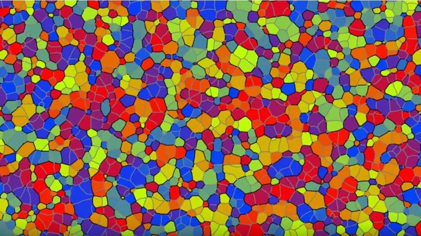
Preprints (www.preprints.org) | NOT PEER-REVIEWED | Posted: 5 August 2021 doi:10.20944/preprints202108.0129.v1 5 of 54 adays a variety of simulation tools in the area on materials simulation draws on this concept e.g. [61],[62],[63] and renders the evolution of complex structures and patterns - in- cluding the dynamics of boundaries and triple junctions - possible, Fig 1. Instructive re- views of phase-field modelling are available e.g. in [64], [65]. Fig. 1: Grain Growth Process: Changes in connectivity and in cardinality of the system occur. The initial grain structure (top) evolves towards the grain structure at a later stage (bot- tom). This grain growth process has been simulated using [61] and a full video of this simula- tion is available in HD resolution [66]. 3.2. Basic Introduction to Phase-Field Models The phase field model in a first place is a way to mathematically describe things and their complex geometrical shape at all, Fig 2. Fig. 2a: A solid phase s (green center region) Fig. 2b: In above tiny volume “1” the frac- coexisting with a liquid phase l (blue outer re- tion solid s amounts to exactly 1, while the gion) in a volume. The fraction solid s amounts fraction liquid l is exactly 0. In the tiny to approx. 1/3 of the overall volume, while the volume “3” the fraction solid s amounts to fraction liquid is approx. 2/3. Both are non-zero exactly 0, while the fraction liquid l is and their correlation (yellow) thus exists as a exactly 1. In contrast, both fractions are boundary in the overall volume. Nothing can non-zero and their correlation (yellow) however be said about the position of this exists in the tiny volume “2”, which thus boundary without further discretization of the comprises a boundary. volume (Fig. 2b).
Preprints (www.preprints.org) | NOT PEER-REVIEWED | Posted: 5 August 2021 doi:10.20944/preprints202108.0129.v1

 6 of 54

 Similar to the Heaviside function Θ(x) [67], the phase-field function in one dimen-
 sion Φ(x) is a function describing the presence or the absence of an object. In contrast to
 the Heaviside function the phase field function, however, reveals a continuous transition
 over a finite —though very small— interface thickness η, Figure3.

 Figure 3: Schematic view of the phase-field function Φ(x). This function takes a non-zero
 value wherever the object is present, it takes exactly the value 1 where it is the only pre-
 sent object and is 0 elsewhere (i.e. where the object is absent). It exhibits a continuous
 transition between two regions over a finite interface thickness η. The Heaviside function
 Θ(x0) being characterized by a mathematically sharp transition at x0 is shown as a refer-
 ence. The dotted region “1” exemplarily corresponds to tiny volume “1” in Fig 2b) where
 only the solid is present.

 Nothing is a priori known about the exact “shape” of the phase field function in the
 transition region. Reasoning towards a specification of this shape is based on statistical
 distributions of gradients in the interface and is described in [68] and [69]. In spite of not
 knowing this exact shape, a number of terms/expressions can already be qualitatively
 identified, Table 1, which all allow the identification and description of the transition re-
 gion (expressions (5), (6), (7 :”overlap”), (8), (13) and (14) in table 1), Figure 4.

 Figure 4: The solid lines represent the three terms occurring in the square of the basic
 equation (expression 12 in Table 1).

 An important characteristic of the phase-field description is that the terms (in ex-
 pressions (4) and (12) in Table 1) corresponding to the “underlap” in mereology (expres-
 sion (3)) sum up to a value of 1 everywhere and any time. Expressed in words expression
 (4) reads:
 The whole is the sum of its fractions
Preprints (www.preprints.org) | NOT PEER-REVIEWED | Posted: 5 August 2021 doi:10.20944/preprints202108.0129.v1 7 of 54 – anywhere, at any time and in any subsystem. Expressed as a formula this reads: 1= ( , ) ( ) with N being the number of things and 0 being the matrix/background thing [1]. In detail this equation - which has a very strong relation to the “mereological sum” defined in mereotopology (see section 4) - means (i) that at least one thing is always present – i.e. has a non- zero value, (ii) that if a thing is the only - single - thing it takes the value of exactly 1 (and all others take exactly the value 0), (iii) that if multiple things exist (i.e. have non-zero values), none of them reaches the value of 1, (iv) that if multiple things exist also their correlations exist (expression 12) and (v) that if multiple things exist (i.e. have non zero values) the sum of all their values equals to 1. Any transformation, any evolution, any mereotopological description is subject to this “normalization” constraint.
Preprints (www.preprints.org) | NOT PEER-REVIEWED | Posted: 5 August 2021 doi:10.20944/preprints202108.0129.v1

 8 of 54

 Table 1: Quantification of boundaries
 in simple phase-field models.
 Expressions (3) and (7) indicate
 links/correspondances to mereology.

 Expression/ variable/ Value in Value in Value in
 remarks
 Term ID term bulk 1 boundary bulk 0

 (1) 1 0
Preprints (www.preprints.org) | NOT PEER-REVIEWED | Posted: 5 August 2021 doi:10.20944/preprints202108.0129.v1 9 of 54 at some – also existing –places xn, xl, which are tiny, but finite volumes inside the region of interest: ≡ ∃ ∧ ( ) ≠ 0 ≡ ∃ ∧ ( ) ≠ 0 ≡ ∃ ℎ ℎ ( ) ≠ 0 ∧ ( ) ≠ 0 This expression describes the collocation of two things in a tiny volume x0. It is equivalent to a non-vanishing algebraic product describing the spatial correlation ik in that tiny volume (see Table 1): → ( ) ( ) ≠ 0 The boundary between these two things thus can be defined as the set of all those volume elements xn in which this correlation does not vanish. Summing up all these non-vanishing spatial correlations over all Nx tiny volumes xn constituting the overall volume of the system under consideration yields the fraction, which the dual boundary between i and k takes of that total volume: 1 ∂ , = ( ) ( ) The symbol " ∂" has been introduced here to denote a boundary. This symbol is typically used in mathematics to denote the boundary ∂ of a region (see also intro- duction of this notation in table 1). The boundary between two things i,k – which is a volume - is related to the sum of all volume elements x n where correlations between thing i and thing k are non-vanishing. Any of the things may have further boundaries also with other things. The total boundary of thing i then - in lowest order of all its dual bounda- ries - is given by the sum of its dual boundaries with all (∀) other things: 1 ∂ ,∀ = ( ) This is the same as ∂ ,∀ = ∂ , ∂ , being identical to 0 means that no interface at all exists between thing i and thing k : neither in the considered domain, nor in any of its sub-domains, nor in any of its elementary volume elements. 3.3. Multi-Phase-Field Models Classical phase field models – and most other theories of phase-transitions and also most mereotopological approaches - describe the boundary or connection between ex- actly two things (resp. the transition between exactly two states). In many areas of ap- plications, however, situations occur, where three or more things coexist and collocate. An instructive practical example is the so called peritectic reaction occurring during so- lidification of a steel grade, Fig. 5:
Preprints (www.preprints.org) | NOT PEER-REVIEWED | Posted: 5 August 2021 doi:10.20944/preprints202108.0129.v1 10 of 54 Fig. 5: Schematic of a peritectic reaction in a steel grade. Red/green/blue areas indicate regions being occupied by the three phases: austenite () ferrite () and liquid melt (L). Wherever there is only (!) Liquid, no ferrite and no aus- tenite may be present. The phases pairwise coexist and collocate at their dual boundaries. All three phases coexist and collocate at the triple junction in the middle of each picture. The upper right inset (the phase-diagram) indicates that the phases also coexist in the same energy interval (i.e. at the same temper- ature). Note the “Basic Equation” for the three things in the center of the figure. To account for such configurations the multi-phase-field concept has been developed [59], which allows for the description of structures comprising multiple objects/things like different phases as depicted in Fig 5. or for multiple grains of a single phase as depicted in Fig. 1. In this multi-phase-field model the basic equation enters as a constraint into the Lagrange density forming the basis for the derivation of the evolution equations for the different phase-fields. 3.4. Triple junctions Higher order junction terms correspond to correlations of three (for triple junctions) or even more things (further, higher order junction terms). In multi-phase-field models triple junction terms are necessary to describe the equilibrium wetting angles like e.g. formed by a droplet on a solid substrate placed in air satisfying “Young’s Law” [70] and especially the kinetics of motion of such triple junctions. A detailed analysis of triple junctions and their role in phase-field models in microstructure evolution is given in [71]. As triple junctions are relevant for the description and discussion especially of “contacts” in the RCC and in mereotopology in section 4, they are explicitly formulated here. For this purpose the basic equation (expression (4) in table 1) has to be formulated for at least three things and has to be – at least – cubed. Simple squaring of the basic equation even for three things will not generate triple junction terms. 1= + + = + + + + + + (+ ⋯ + ⋯ + ⋯ , , ) The volume term (first term of the RHS) for the bulk fraction, where only the one object i exists then reads
Preprints (www.preprints.org) | NOT PEER-REVIEWED | Posted: 5 August 2021 doi:10.20944/preprints202108.0129.v1 11 of 54 1 ∂ = ( ) The dual boundary fractions (2nd and 4th term for i,k, resp. 3rd and 5th term for i, j) for the region i with the other region k in this ternary case then read: 1 1 ∂ , = ( ) ( ) + ( ) ( ) This expression reduces to the binary case if j =0: ∂ , = ( ) ( ) ( ) + ( ) ( ) ( ) ∂ , = ( ) ( ) ( ) + ( ) ( ) ( ) ∂ , = ( ) ( ) [ ( ) + ( )] with the sum in the square brackets being equal to 1 if j=0: ∂ , = ( ) ( ) The two ternary terms – the triple junction terms 6 and 7 on the RHS of the equation - contributing to the boundary of region i read: ∂ , , = ( ) ( ) ( ) and ∂ , , = ( ) ( ) ( ) These two terms –being permuted in the last two indices- correspond to two dif- ferent types of triple junctions revealing a different helicity. The topic helicity is dis- cussed in a separate section below. The total boundary of a thing i then is the sum of its dual boundaries plus the triple junction terms: ∂ ,∀ = ∂ , + ∂ , , , Based on the these specifications of boundary and triple junction terms, mereotop- ological relations can be easily be formulated and visualized based on some simple con- figurations as will be shown in section 4. It is important to note that all current mereo- topological relations between two things will probably profit from the introduc- tion/notion of a third thing, the “background” or “matrix” thing 0, to which they are connected as well, Fig. 6.
Preprints (www.preprints.org) | NOT PEER-REVIEWED | Posted: 5 August 2021 doi:10.20944/preprints202108.0129.v1

 12 of 54

 No triple junction: One triple junction: Two triple junctions:
 1 isDisconnected 2 1 isExternalContact 2 1 isPartOf 2
 Figure 6: Classification of different configurations known from mereotopology and re-
 gion connect calculus according to the number of triple junctions being present in the
 system. Dyadic relations between two things turn into triadic relations of three things if
 the matrix thing (0) is taken into account.

 The simple examples depicted in Fig. 6 are introduced here to highlight the role of
 the “background” resp. “matrix” thing “0” and also the importance of triple and higher
 order junctions for mereotopology in general. The class “no triple junction” besides the
 case “isDisconnected” also contains the case “isNonTangentialProperPart”, the class “one
 triple junction” applies to “isExternalContact” and also to “isTangentialProperPart”. Even-
 tually the presence of two triple junctions corresponds to the “isPartOf” relation.
 Additional remark: The three configurations of things depicted in Fig. 6 might also
 be considered as a temporal sequence of two individuals (“atoms”) being initially dis-
 connected and then entering into a bound state. This scenario relates to Mulliken’s holis-
 tic interpretation of a bound state [72], where the two atomic orbitals must incorporate
 “the overlap in the space region that corresponds to the intersection of each atomic
 space” [73]. A mereology of quantum chemical systems has recently been discussed [74].

 Fig.7 a: Multiple things in a volume. The
 two situations left can be described well
 by classical mereotopology. Most left: All
 things are mutually disconnected resp
 connected with the matrix only.
 Left: 1 isPartOf 3,
 2 isDisconnected from both 1 and 3

 Fig 7b: Configurations not typically being described by classical mereotopology. They
 differ in number and type of triple junctions. This number increases from 4 (left) to 6
 (middle) all of which include the matrix thing. Eventually (right) a situation of 4 triple
 junctions is possible in which one of these triple junctions does not comprise the matrix
 thing. Note that the number of triple junctions is always even. The case of “external
 contact” seemingly having only one triple junction is discussed separately (see text).

 In case all three things being connected to each of the other things (see Figure 7
 lower right and Figure 8) there are three dual boundaries. Starting from the bottom and
 crossing these boundaries counter-clockwise, Figure 8 (left) gives following sequence:
 red-blue , blue-green , green-red, which we abreviate for the ease of further reading as
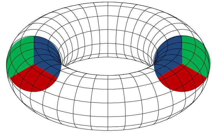
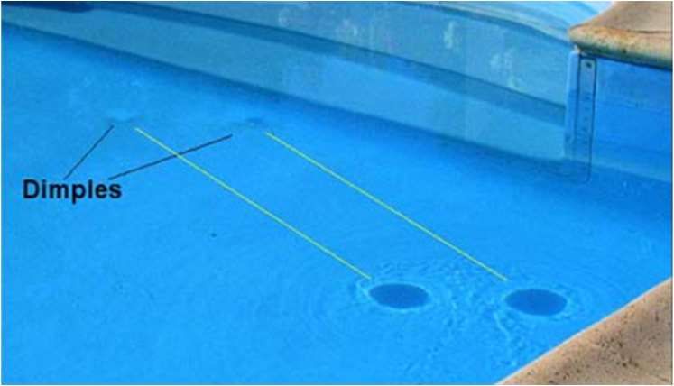
Preprints (www.preprints.org) | NOT PEER-REVIEWED | Posted: 5 August 2021 doi:10.20944/preprints202108.0129.v1

 13 of 54

 R-B, B-G, G-R or even simpler (omitting also the hyphons) as RB, BG, GR. Thus “RB”
 reprents a transition from red to blue. This is definitely something to be distinguished
 from a transition “BR” going from blue to red. RB thus is not the same as BR. The
 sequence of the symbols being used to denote the boundary thus is important and has a
 meaning. It denotes the direction in which the boundary is crossed. Taking the
 convention of reading letters from left to right (as usual in most western languages) one
 will start from red to blue. In contrast, when taking the convention of reading signs from
 right to left (as e.g. in Arabian language) the red to green transition would be the first.
 Even more interesting is to have a look at the sequence when going from one area to the
 next neighboring area. Again starting on the bottom (the red region in Fig.8) the sequence
 reads R-B-G (and eventually back to red: -R). But one could also start from blue and
 continue in so- called cyclic permutations :

 R-B-G is the same as B-G-R is the same as G-R-B

 One will however never end (for this triple symbol AND when continuing going
 clockwise! ) in a situation:

 R-G-B is the same as G-B-R is the same as B-R-G

 The sequence of letters used to describe these two symbols - in 2 dimensions - thus
 either allows (i) distinguishing two different types of triple junctions or (ii) describing a
 sense of rotation (clockwise/counterclockwise), Fig. 8 (left) and Fig. 8 (right).

 Figure 8 : Two different triple juntions in 2 dimensions in which three objects red (R),
 green (G), and blue (B) coexist and collocate. They can be distinguished by the
 sequence in which the three things are arranged. They cannot be mapped onto each
 other by any rotation in 2D (see text), but only by mirroring. They may be – and in 3D
 physical systems probably are – connected in the third dimension (see text and Fig.
 10) meaning that they are parts of the same thing.

 Triple junctions are regions of collocation of three things. They are also regions
 where the three dual boundary planes (which each are volumes being thin in one
 direction) between the three differnet things collocate. As boundaries between any pair of
 two things in 3D are “planes”, the intersection of any pair of “planes” defines a “line” In
 three dimensions. Triple junctions thus are “lines” (having finite volumes), which in 3
 dimensions either form closed loops - called vortices - or are connected to the boundary
 of the region of interest, respectively. Triple junctions are not “points” as they seem to be
 in a 2 D section, but lines. In 2D sections they always appear as “pairs”, Figure 9.
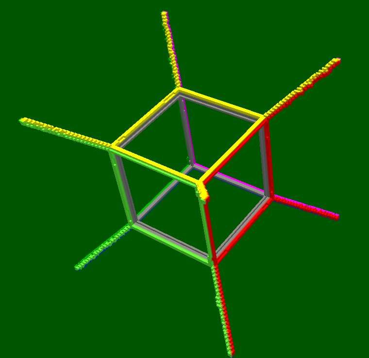
Preprints (www.preprints.org) | NOT PEER-REVIEWED | Posted: 5 August 2021 doi:10.20944/preprints202108.0129.v1 14 of 54 Fig.9a) Visualisation of a vortex resp. of a Fig.9b) Smoke vortices as propagaing torus. A 2D section reveals two vortcies objects in a 3D world. Photo with opposite helicities. reproduced from [75] Fig.9c) Triple junctions in a 2 D section Fig. 9d) Experimental visualisation of at the water surface always show up as 3-D conectivity of two vortices [78]. The pairs, shown here for two flow vortices surface dimples have been couloured (“dimples”) in a pool - so called Falaco with green fluid, which reveals them solitons [76]. “Falaco solitons appear to being coupled in the third dimension in have properties claimed by the String a semi vortex extending under the water theorists trying to explain Quantum surface. Gravity” [77]. 3.5. Quadruple and higher order junctions A maximum of 4 things can coexist at the same position “i.e. coexist and collocate”. In such a case they form quadruple “points”. Such quadruple points only exist in 3D space. Remember that all “points”, “lines” and “planes” are 3D objects (in a 3D world) resp. 4D objects in a 4D world (see Appendix A). There are o pairs of things forming dual boundaries ( being “planes”) o 3 coexisting/collocated things forming 3 dual boundaries being coexisting/ collocated in a triple boundary (being a “line”) o 4 coexisting things have following boundaries as parts 1 quadruple “point”, 4 triple “line” junctions, and 6 dual boundary “planes” The fourth power of the basic equiation for 4 things yields total of 44 = 256 terms and can be sorted using the multinomial expansion6: 4! ( + + + ) = 1! 2! 3! 4! The ki always sum up to 4 by definition of the sum. This is further detailed in Appendix C and eventually allows classifying into 4 “unary” terms ∂ with one ot the ki equals 4 and the others are identical 0 6 see e.g https://en.wikipedia.org/wiki/Multinomial_distribution
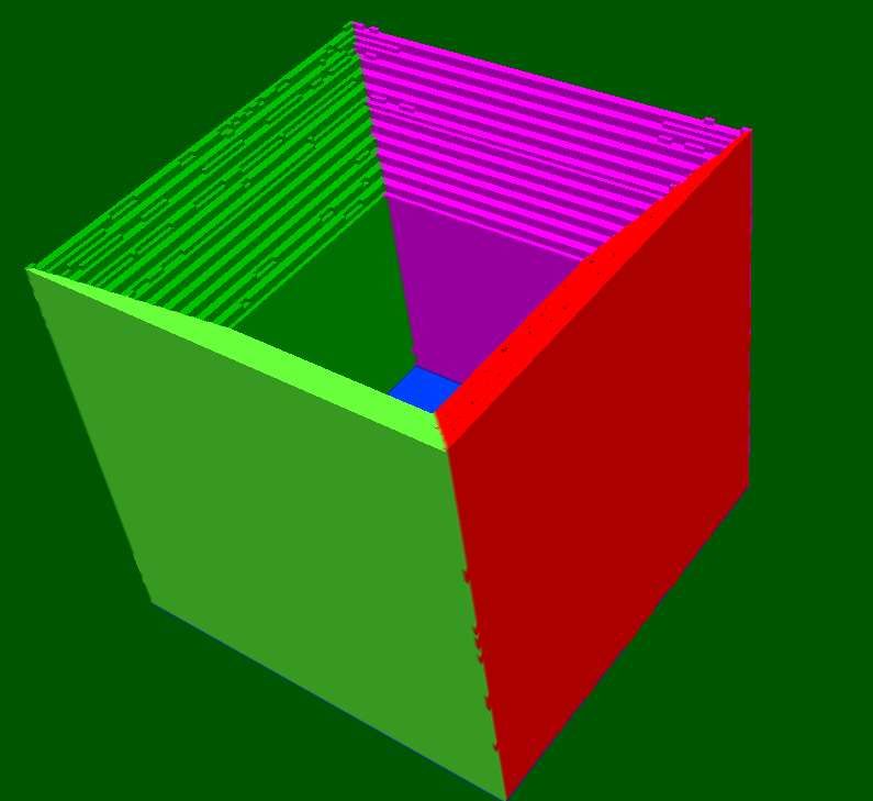
Preprints (www.preprints.org) | NOT PEER-REVIEWED | Posted: 5 August 2021 doi:10.20944/preprints202108.0129.v1 15 of 54 84 “dual” boundary terms, where two of the ki are identical 0 and the others complement to 4. For a dual boundary i,j this provides 14 terms: ∂ , (7terms) and ∂ , (7terms). A total of 6 boundary pairs (i,j; i,k; i,l; k,l; j,k and j,l) thus generates the total of 84 dual boundary terms. 144 “triple” boundary terms, where one of the ki is identical 0 and the three others complement to 4. Each triple junction i,j,k generates 36 terms, which can be classified according to the helicity of the junction: ∂ , , (18terms) + ∂ , , (18 terms) = ∂ , , (36 ) A total of 4 triple sets (i,j,k; i,j,l; i,k,l and j,k,l) thus generates the total of 144 triple boundary terms. 24 “quadruple” boundary terms, where all ki are identical 1 leading to (sorted by first index) ∂ , , , (6 ); ∂ , , , (6 ); ∂ , , , (6 ); ∂ , , , (6 ) In summary the following overall equation scheme results: = ∂ + ∂ , + ∂ , , +∂ , , + ∂ , , , , , , = ∂ + ∂ , + ∂ , , +∂ , , + ∂ , , , , , , = ∂ + ∂ , + ∂ ,, +∂ , , + ∂ , , , , , , = ∂ + ∂ , + ∂ , , +∂ , , + ∂ , , , , , , 1= ∂ + ∂ , + ∂ , , +∂ , , + ∂ , , , , , , , This eventually yields the total fractions of the 4 different objects (the LHS) as these are summed up from contributions of bulk, dual, triple and quadruple boundaries. A visual impression of the different terms for bulks, dual boundaries, triple and quadruple junctions is depicted in Fig.10.
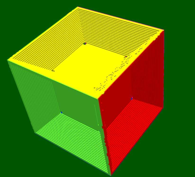
Preprints (www.preprints.org) | NOT PEER-REVIEWED | Posted: 5 August 2021 doi:10.20944/preprints202108.0129.v1 16 of 54 Fig.10: Volumes, Faces/Areas, Egdes/Lines and Vortices/Quadruple Points in a tesseract cube. Upper row: ouside view of the tesseract (left), center cube and one of the faces removed (middle) and dual boundaries (right). Lower row: triple lines (left), quadruple points (middle) and zoom-in into a quadruple point (right). The tesseract structure was synthesized using [61]. 3.6. Summary of phase-field expressions In view of the comparison with expressions from Region Connect Calculus, from Contact algebra and from mereology in the following sections, Table 2 provides a list of all terms being necessary for this purpose. equation global local value in relation global-local # value volume xn 1 1 ( ) = ( ) 1 2 ∂ ∂ ( ) ∂ = ∂ ( ) 1 3 ∂ , ∂ , ( ) ∂ , = ∂ , ( ) 1 4 ∂ , , ∂ , , ( ) ∂ , , = ∂ , , ( ) 1 5 , , , , , , ( ) , , , = , , , ( ) 6 ∂ ,∀ n/a ∂ ,∀ = ∂ , Table 2: List of all terms being necessary to express mereotopological and region connect calculus situations. The quadruple terms seem not yet to be needed to address the mereotopological situations being investigated in the literature by now. Looking at possible extensions to higher order expressions questions emerge like: Why not raising the basic equation to the 6th , to the 8th or even higher powers? Is an even power mandatory? Why not go for more than 4 different objects? For small number of objects (one or two or three) an exponent being equal to the number of objects seems sufficient. If only two objects exist, there will be no triple junction and an exponent of 2 can be considered as sufficient. As a first rule of thumb the exponent thus should correspond to the number of objects. An exponent of 4 then seems sufficient – and necessary - to describe all types of geometric coexistence regions (dual boundaries “planes”; triple junctions “lines” and quadruple junctions “points”) even if multiple
Preprints (www.preprints.org) | NOT PEER-REVIEWED | Posted: 5 August 2021 doi:10.20944/preprints202108.0129.v1 17 of 54 objects are collocated. A power of 6 was used in [66] to refine the desription of the dual interface in a solid-liquid two state system by a refined discretisation. 4. Comparison with mereotopological concepts Based on the specifications of bulk areas, boundaries, triple junctions and quadruple junctions depicted in the preceding section, especially in Table 2, mereotopological rela- tions can easily be formulated and visualized based on some simple configurations as outlined in the following. 4.1 Comparison with Region Connect Calculus Some simple Region Connect Calculus (RCC) situations, Fig.11, are individually discussed based on the description of boundary terms as introduced in section 3. Starting from the easily identifiable configurations (X DC Y, X NTTPi Y, X NTTP Y, and X PO Y), the more complex situations involving only one Triple Junction (X EC Y, X TPP Y, X TPPi Y) are discussed. Most attention is paid to the case X EQ Y. Fig. 11 : Region Connection Calculus7: disconnected (DC), externally connected (EC), equal (EQ), partially overlapping (PO), tangential proper part (TPP), tangential proper part inverse (TPPi), non-tangential proper part (NTPP), non-tangential proper part inverse (NTPPi) Case: X DC Y: X and Y do not have any common boundary: , =0 For X DC Y, parts X AND Y both have boundaries with the background thing 0 (not shown in the figure) only. Their total boundary thus hasPart only the boundary to the thing 0: ,∀ = , ,∀ = , As there exists no dual boundary between X and Y, also no triple junctions involving either of the two parts do exist: , , = 0 ⋀ , , = 0 ⋀ , , = 0 ⋀ 7 https://en.wikipedia.org/wiki/Region_connection_calculus
Preprints (www.preprints.org) | NOT PEER-REVIEWED | Posted: 5 August 2021 doi:10.20944/preprints202108.0129.v1 18 of 54 , , =0 Case: X NTPP Y: X has a boundary with Y only while Y has a boundary to thing 0 in addition: ,∀ = , ,∀ = , + , Although there exists a boundary between both things, there is no region where both things are connected to the 0-thing as well. Thus there are no triple junctions: , , =0 ⋀ , , =0 ⋀ , , =0 ⋀ , , =0 Case: X NTPPi Y: Y has a boundary with X only while X has a boundary to thing 0 in addition: ,∀ = , + , ,∀ = , Though there exists a boundary between both parts, there is no region where both things are connected to the 0-thing as well. There are no triple junctions: , , =0 ⋀ , , =0 ⋀ , , =0 ⋀ , , =0 All these three cases above do not comprise any triple junction. The easiest case in- cluding triple junctions (X PO Y) will be discussed first as this discussion is helpful in understanding the cases revealing one single triple junction only (i.e. the cases X EC Y, X TPP Y, X TPPi Y) Case: X PO Y: X and Y reveal a region of coexistence/collocation –the overlap region. A boundary between X and Y thus exists: , >0 Further, both things X and Y in this case also have boundaries to thing 0: , > 0 , > 0 X PO Y further comprises two regions (“points”) where all three things X AND Y AND the 0-thing collocate: there exist two triple junctions. Their total boundary thus hasPart the boundaries to thing 0, to X (resp. to Y) and further the two triple junctions where X, Y and 0 coexist/collocate. These two triple junctions however do NOT collocate - i.e. they exist in different volumes xl and xm - and are distinguished by different helici- ties for the two different locations, see section 3.4. A correlation of the two triple junctions does not exist in any volume element xn: ,∀ = , + , + , , + , , ,∀ = , + , + , , + , , ∃ : , , ( ) ≠ 0 ⋀ ∃ : , , ( ) ≠ 0 ⋀ ∀ : , , ( ) , , ( ) = 0
Preprints (www.preprints.org) | NOT PEER-REVIEWED | Posted: 5 August 2021 doi:10.20944/preprints202108.0129.v1 19 of 54 Case: X EC Y In this case there seemingly exists a single triple junction in a discretized single volume xn. This defines a “point” (a finite sized smallest volume in 2 dimensions....) , , >0 In the case X PO Y discussed above, two triple junctions are coexistent - but not collocated. In the case X DC Y no triple junctions are existent. X EC Y describes a transi- tion between X DC Y and X PO Y and thus benefits from being capable of describing both cases – each of them as a limit. Looking at the reverse process the two separated – i.e. not collocated - triple junctions in the X PO Y case then have to condense in to a single state of coexistence AND collocation for the X EC Y case ( and also for the TPP cases..) ∃ : , , ( ) ≠ 0 ⋀ , , ( ) ≠ 0 → ∃ : , , ( ) , , ( ) ≠ 0 Case: X EQ Y X and Y obviously have the same total boundary: ,∀ = ,∀ Both have a boundary with 0 only ,∀ = , ,∀ = , Further, they both have identical phase fields, ∀ : ( ) = ( ) This expression directly implies that the two things are identical i.e. the “same thing” in a mereological sense. They have the same geometry as defined by their indi- vidual phase fields. In terms of being fractions of a universe both things are also identical. They can be treated as a single thing representing twice the fraction of one of the two things but losing their identity then: ∀ : ( ) = ( ) + ( ) = 2 ( ) Further, there may be additional attributes beyond the mere geometric shape, which may still allow distinguishing them in spite of being geometrically identical. 4.2 Phase-Field perspective of Contact Algebra The topology axioms of contact algebra are (adapted from [18]): (C1) If aCb, then a > 0 and b > 0, (C2) If aCb and a ≤ c and b ≤ d, then cCd, (C3) If aC(b + c), then aCb or aCc, (C4) If aCb, then bCa, (C5) If a●b≠ 0, then aCb. In the following these axioms are related and compared to the phase-field formula- tions for time independent situations. The phase-field formulations introduced in the
Preprints (www.preprints.org) | NOT PEER-REVIEWED | Posted: 5 August 2021 doi:10.20944/preprints202108.0129.v1 20 of 54 preceding section are shortly recovered in the following for this purpose. A thing a is globally present in a region under consideration if it takes a non-zero value in this region: >0 A thing a is locally present in a region xj, which is a sub-region of the region under consideration, if it takes a non-zero value in that sub-region ( ) > 0 The global value a of is the normalized sum of all local values in the Nx sub-regions 1 = ( ) Eventually the definition of “collocation” is: ≡ ∃ ℎ ℎ ( ) ≠ 0 ∧ ( ) ≠ 0 which implies that there exists a boundary between the two things → , ≠ 0 “Collocated” in this context (i.e. time independent) means “isSpatiallyConnected” or just isConnected i.e. in the nomenclature of contact algebra. The Axiom (C1) of Contact Algebra -using these phase-field definition of isSpatially- Connected – then translates into ≡ , ≠0 , ≠ 0 → ∃ ℎ ℎ ( ) ≠ 0 ∧ ( ) ≠ 0 ( ) ≠ 0 → ≠0 → ≠0 ( ) ≠ 0 → ≠0 → ≠0 → ≠0 ∧ ≠0 Expressed in words this reads “If two things are locally connected, both things must at least globally exist”. Axiom (C1) thus is recovered by the phase field perspective. Axiom (C3) covers the case of one thing being connected to two other things, which both globally exist: ≠0 ∧ ≠0 ∧ ≠0 ( + ) → ∃ ℎ ℎ ( ) ( ) + ( ) ≠ 0 ( ) ( ) + ( ) ( ) ≠ 0
Preprints (www.preprints.org) | NOT PEER-REVIEWED | Posted: 5 August 2021 doi:10.20944/preprints202108.0129.v1 21 of 54 → ( ) ( ) ≠ 0 ∨ ( ) ( ) ≠ 0 → , ≠ 0 ∨ , ≠0 → ∨ Expressed in words this reads “If a thing is connected to two other things, it is con- nected to at least one of them”. Axiom (C3) thus is recovered also by the phase field perspective. For multiple things this can even be even further refined as: “Any thing is connected to at least one of the other things” or “Any thing is connected to its comple- ment”. Axiom (C4) relates to the symmetry of the connected relation ≡ ∃ ℎ ℎ ( ) ≠ 0 ∧ ( ) ≠ 0 ( ) ≠ 0 ∧ ( ) ≠ 0 → ( ) ≠ 0 ∧ ( ) ≠ 0 ( ) ≠ 0 ∧ ( ) ≠ 0 → Expressed in words this reads: “If thing “a” is connected to thing “b”, then thing “b” is also connected to thing “a””. Axiom (C4) thus is recovered also by the phase field perspective for time - independent correlations. The situation however may be – and probably is – different for time dependent and other situations. A “path” connecting two things “a” and “b” may exist for some time, while the return path might not exist anymore, when attempting to go back from “b” to “a”. An example would be a bridge connecting “a” and “b”, which breaks down when crossing it for the first time. The concept of asymmetric connectivity has major implica- tions for a number of areas in physics and chemistry like chemical reactions preferen- tially proceeding into one direction, entropy always increasing or osmotic processes to name a few. A simple example from everyday life is a one-way in traffic. To the best of the author’s knowledge a concept of asymmetric connectivity has not yet been discussed in any of the contemporary mereotopology endeavors. “Symmetric connectivity” can be retained by defining two things a,b as isConnected if at least one path direction does exist. This allows for a more general – even symmetric - formulation: a, b are connected a isPathConnected b ∨ b isPathConnected a This expression, which still is symmetric, can be satisfied by following three con- figurations: a isPathConnected b ∧ b ¬ isPathConnected a a ¬ isPathConnected b ∧ b isPathConnected a a isPathConnected b ∧ b isPathConnected a The last expression indicates the existence of a reversible path, while both other ex- pressions lead to irreversible situations, where there is a path from “a” to “b” (or vice versa) but no way back. Path connectivity is an important concept being introduced by Richard P. Feynman and finds applications in the principles of least action and/or Fer- mat’s principle. It is discussed in a little more detail in section 5.5. In a last but one step Axiom (C5) is discussed, which essentially states that if two things globally exist, they are connected:
Preprints (www.preprints.org) | NOT PEER-REVIEWED | Posted: 5 August 2021 doi:10.20944/preprints202108.0129.v1 22 of 54 ≠0 ∧ ≠0 → ≠0 1 1 ⎛ ⎞ = ( ) = ( ) + ( )⎟ ≠ 0 ⎜ , ⎝ ⎠ The second sum contains correlations between the volume elements xj and xk of the reference frame when re-expressing the fields as products . . ≡ ; see Appendix B5 . Neglecting such correlations (i.e. = 0 for all i,j) the second 8 term on the RHS vanishes and only the first sum remains: ≠0 → ( ) ( ) ≠ 0 ( ) ( ) ≠ 0 → , ≠0 , ≠0 → Expressed in words this reads “If two things globally exist, they are connected”. Axiom (C5) thus is recovered also by the phase field perspective for the case of exactly two coexisting things. However, for three (and more things) existing globally, i.e. for ≠0 ∧ ≠0 ∧ ≠0 a number of options occurs, which can be identified when using Axiom (C3): ( + ) ≠ 0 → + ≠ 0 → ≠ 0 ∨ ≠ 0 → ∨ Thus - even in case two things a and b do exist globally (i.e. have non-zero values) – these two things a and b do not necessarily need to be connected if more than two things are globally present. In case “a” and “b” not being mutually connected, both have to be connected to – or separated by - a third thing c. This directly implies the following global relations ≠0 ∧ ≠0 ∧ ≠0 → , ≠ 0 ∨ , ≠ 0 ∨ , ≠ 0 Expressed in words this reads “If three things globally exist, each of them is con- nected to at least one of the two other things”. While two things being mutually con- nected directly implies that both exist globally (see Axiom C1): → ( ) ( ) ≠ 0 → ≠ 0 their individual global existence – in contrast however – does NOT imply that they are connected if more than two things are considered. In case of three things a,b,c two of them 8 In the spirit of the present article such correlations will exist between volumes being in contact with each other i.e between neighboring positions. They are neglected here to show under which conditions the axioms of Contact Algebra can be recovered. These terms open options for a future refinement of the concept.
Preprints (www.preprints.org) | NOT PEER-REVIEWED | Posted: 5 August 2021 doi:10.20944/preprints202108.0129.v1 23 of 54 e.g. a,b may be mutually connected or may be disconnected (i.e. separated by the third thing c then): ≠ 0 → , ≠ 0 ∨ , = 0 , = 0 → ¬ In case one of these boundaries does NOT exist (i.e. equals to 0) both other boundaries must exist (i.e. take non-zero values): , = 0 → , ≠ 0 ∧ , ≠0 In the case a triple junction exists, all three dual boundaries do exist: , , ≠ 0 → , ≠ 0 ∧ , ≠ 0 ∧ , ≠0 Axiom (C5) of Contact Algebra thus is recovered for exactly two existing things. The phase-field perspective depicted above seems however to imply that this axiom might have to be re-considered for the case of more than two things. Eventually Axiom (C2) will be discussed. This seems the most complicated discus- sion as it involves 4 different things. The axiom (C2): “if aCb and a ≤ c and b ≤ d, then cCd” expressed in words reads: If a isConnected b and a isPartOf c and if b isPartof d then c isConnected b. The individual expressions formulated in phase-field boundary terms translate into → , ≠ 0 If a isPartOf c, there exists a boundary between a and c: ≤ → , ≠0 The total boundary of “a” then hasPart the 2 dual boundaries, but inevitably then also comprises a triple junction a,b,c ,∀ = , + , + , , Then further b isPartOf d implies the existence of a boundary between b and d ≤ → , ≠0 The total boundary of “b” then hasPart the 2 dual boundaries, but inevitably also a triple junction a,b,d: ,∀ = , + , + , , If aCb ℎ ≡ ∃ ℎ ℎ ,∀ ( ) ≠ 0 ∧ ,∀ ( ) ≠ 0 , , ≠ 0 ∧ , , ≠ 0 → , , , ≠ 0 → , ≠ 0 → Accordingly also Axiom C2 can be recovered by the phase field perspective. In summary, all five axioms of the axiomatic system of contact algebra can be expressed in terms of dual and higher order boundaries as described by the phase-field perspective.
Preprints (www.preprints.org) | NOT PEER-REVIEWED | Posted: 5 August 2021 doi:10.20944/preprints202108.0129.v1 24 of 54 4.3 Comparison with Mereology While “connections” as used in Region Connect Calculus and topology have been de- scribed as “boundaries” between things in the preceding chapter, the description of a “part” being at the heart of mereology is related to the phase-field itself in the phase field perspective. The section starts with a short overview of mereology as being described in detail in [2]. 4.3.1 Mereological Axioms and Definitions Part: The monadic relation ≡ defines “x” to be a part. This expression implies the existence of “x” as in order to be a part “x” must exist. It finds its phase-field counterpart in the expression 9 ≡ ≠0 which implies “a” (denoted as in the phase-field perspective) to be a non-zero fraction of a system under consideration. The thing exists if it has a non-zero value, in case the thing does not exist it takes exactly the value 0 [46]: ≡ ≠ 0 ≡ = 0 Parthood: Mereology further builds on a dyadic relation specifying parthood: ≡ This parthood relation is considered as primitive following some basic axioms like (see e.g. [2]): ( ) ∧ → = ( ) ∧ → ( ) Some commonly used definitions based on these axioms are O ≡ ∃ ( ∧ ) ( ) U ≡ ∃ ( ∧ ) ( ) PP ≡ P ∧ ¬ P ( ℎ ) Above axioms of Ground Mereology (M) are further complemented by a strong supplementation in Extensional Mereology (EM): ¬ P → ∃ ( ∧ ¬ ) ( ) Extensional Mereology then is further complemented by following closure exten- sional axioms leading to Closure Extensional Mereology (CEM): U → ∃ ∀ ( ↔ ( ∨ )) ( ) O → ∃ ∀ ( ↔ ( ∧ )) ( ) 9 by intention the phase field notation will deviate from using “x” to denote a part as usual in mereology. In the context of the phase field perspective, a,b,c etc will be used instead. This is to avoid confusion with the xi being used to denote elementary spatial regions in the phase field perspective.
Preprints (www.preprints.org) | NOT PEER-REVIEWED | Posted: 5 August 2021 doi:10.20944/preprints202108.0129.v1 25 of 54 ∃ ∀ ( ) Specifying a particular, individual z matching the upper bound axiom fixes a uni- verse under consideration having part all parts: ≡ ∃! ∀ ( ) 4.3.2. An essay towards a first order logic description of the phase-field concept The phase-field method to the best of knowledge of the author by now has not been formulated as an axiomatic system. The following section thus can be considered as a first essay towards formalizing the phase-field concept. It does not reveal the degree of maturity of the mereological axioms and is subject to future review. Before formu- lating the phase-field concept in FOL it is instructive to summarize the major concepts in their algebraic form. In the phase-field concept all existing things are fractions and sum up to form the “whole” (i.e. the value 1). Not-existing things do not contribute to this sum as their values are identical 0. + =1 The “complement thing” has been added to this sum to account for all un-named or un-identified - but existing - fractions of the universe. The “complement thing” accordingly can be defined as: ≡ 1− The result is the “basic equation” already being introduced in [1] with the summa- tion starting from i=0: = 1 ( ) Without rigorous proof – which is beyond the scope of the present article - a number of implications can directly be inferred: (i) postulating the number of things to be finite (N) directly implies the existence of a smallest fraction which has no parts (i.e. an “atom”) and of a largest fraction (an “upper bound”) (ii) if a thing is the only thing (the “whole”) it takes the value 1 and its complement is 0 (iii) if a thing is not the only thing, the complement exists (i.e. it has a non-zero value) (iii) the basic equation corresponds to the mereological sum of all existing things (in- cluding the complement) (v) in case both - a thing and its complement thing - exist, their –mereological- product (or their “boundary”, or their “correlation”) does exist and they are connected (see sec- tion 4.2): ¬ = (1 − ) ≠ 0
You can also read