Drivers of Pine Island Glacier speed-up between 1996 and 2016 - The Cryosphere
←
→
Page content transcription
If your browser does not render page correctly, please read the page content below
The Cryosphere, 15, 113–132, 2021
https://doi.org/10.5194/tc-15-113-2021
© Author(s) 2021. This work is distributed under
the Creative Commons Attribution 4.0 License.

Drivers of Pine Island Glacier speed-up between 1996 and 2016
Jan De Rydt1 , Ronja Reese2 , Fernando S. Paolo3 , and G. Hilmar Gudmundsson1
1 Department   of Geography and Environmental Sciences, Northumbria University, Newcastle upon Tyne, UK
2 Potsdam  Institute for Climate Impact Research (PIK), Member of the Leibniz Association, Potsdam, Germany
3 Jet Propulsion Laboratory, California Institute of Technology, Pasadena, CA, USA

Correspondence: Jan De Rydt (jan.rydt@northumbria.ac.uk)

Received: 15 June 2020 – Discussion started: 7 July 2020
Revised: 11 November 2020 – Accepted: 22 November 2020 – Published: 7 January 2021

Abstract. Pine Island Glacier in West Antarctica is among         1   Introduction and motivation
the fastest changing glaciers worldwide. Over the last 2
decades, the glacier has lost in excess of a trillion tons of
ice, or the equivalent of 3 mm of sea level rise. The ongoing     Since the 1990s, satellite measurements have comprehen-
changes are thought to have been triggered by ocean-induced       sively documented the sustained acceleration in ice discharge
thinning of its floating ice shelf, grounding line retreat, and   across the grounding line of Pine Island Glacier (PIG, Fig. 1)
the associated reduction in buttressing forces. However, other    in West Antarctica (Rignot et al., 2002; Rignot, 2008; Rig-
drivers of change, such as large-scale calving and changes in     not et al., 2011; Mouginot et al., 2014; Gardner et al., 2018;
ice rheology and basal slipperiness, could play a vital, yet      Mouginot et al., 2019b). The changes in flow speed are an ob-
unquantified, role in controlling the ongoing and future evo-     servable manifestation of the glacier’s dynamic response to
lution of the glacier. In addition, recent studies have shown     both measurable perturbations, such as calving and ice shelf
that mechanical properties of the bed are key to explaining       thinning, and poorly constrained variations in physical ice
the observed speed-up. Here we used a combination of the          properties and basal sliding. Evidence from indirect observa-
latest remote sensing datasets between 1996 and 2016, data        tions has indicated that changes in ice shelf thickness have
assimilation tools, and numerical perturbation experiments        occurred since at least some decades before the 1970s (Jenk-
to quantify the relative importance of all processes in driv-     ins et al., 2010; Smith et al., 2017; Shepherd et al., 2004;
ing the recent changes in Pine Island Glacier dynamics. We        Pritchard et al., 2012). Within the last 2 decades, thinning
show that (1) calving and ice shelf thinning have caused a        of the grounded ice (Shepherd et al., 2001; Pritchard et al.,
comparable reduction in ice shelf buttressing over the past 2     2009; Bamber and Dawson, 2020), intermittent retreat of the
decades; that (2) simulated changes in ice flow over a vis-       grounding line (Rignot et al., 2014), changes in calving front
cously deforming bed are only compatible with observations        position (Arndt et al., 2018), and the partial loss of ice shelf
if large and widespread changes in ice viscosity and/or basal     integrity (Alley et al., 2019) have all been reported in consid-
slipperiness are taken into account; and that (3) a spatially     erable detail. At the same time, numerical simulations of ice
varying, predominantly plastic bed rheology can closely re-       flow have confirmed the strong link between ice shelf thin-
produce observed changes in flow without marked variations        ning, which reduces the buttressing forces, and the increased
in ice-internal and basal properties. Our results demonstrate     discharge across the grounding line (Schmeltz et al., 2002;
that, in addition to its evolving ice thickness, calving pro-     Payne et al., 2004; Joughin et al., 2010; Seroussi et al., 2014;
cesses and a heterogeneous bed rheology play a key role in        Favier et al., 2014; Arthern and Williams, 2017; Reese et al.,
the contemporary evolution of Pine Island Glacier.                2018; Gudmundsson et al., 2019). Due to the dynamic con-
                                                                  nection between ocean-driven ice shelf melt rates and trop-
                                                                  ical climate variability (Steig et al., 2012; Dutrieux et al.,
                                                                  2014; Jenkins et al., 2016; Paolo et al., 2018), several model
                                                                  studies have focused on the important problem of simulat-
                                                                  ing the response of PIG to a potential anthropogenic intensi-

Published by Copernicus Publications on behalf of the European Geosciences Union.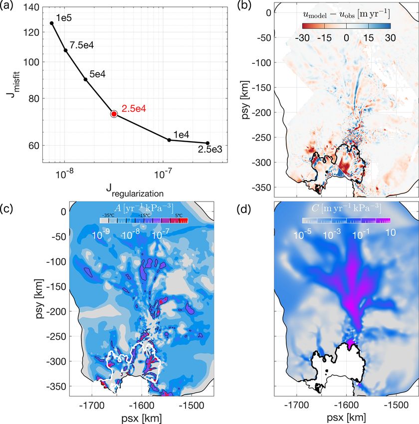
114                                                                             J. De Rydt et al.: Pine Island drivers of change

fication of melt. Such external perturbations, in combination       distribution, is balanced by resistive stresses, which include
with ice-internal feedbacks including the marine ice sheet in-      the basal drag (τ b ), side drag through horizontal shear (τ W ),
stability, can force PIG along an unstable and potentially ir-      longitudinal resistive forces (τ L ), and back forces by the ice
reversible trajectory of mass loss (Favier et al., 2014; Rosier     shelf (τ IS ):
et al., 2020). Whereas significant progress has been made in
                                                                    τ d = τ b + τ W + τ L + τ IS .                               (1)
simulating the melt-driven retreat of PIG, less attention has
been given to other processes that could affect the force bal-      It is conceivable that each of the terms in Eq. (1) has changed
ance and thereby inhibit or foster changes in ice dynamics.         considerably in recent decades in response to changes in
Increased damage in the shear margins of the ice shelf, for         calving front position, ice thickness, ice properties, and/or
example, has been reported by Alley et al. (2019) and Lher-         basal slipperiness. The interplay between different changing
mitte et al. (2020), and is known to reduce the buttressing         forces, in combination with the appropriate boundary condi-
capacity of an ice shelf (Sun et al., 2017). Moreover, a series     tions, underlies the observed speed-up of PIG (1U ). Present-
of recent calving events has led to a sizeable reduction in the     day observations of 1U are generally assumed to be domi-
extent of the ice shelf and caused a potential loss of contact      nated by ice shelf thinning and induced dynamic loss and re-
with pinning points along the eastern shear margin (Arndt           distribution of mass upstream of the grounding line, which
et al., 2018).                                                      includes grounding line retreat and the associated loss of
   The relative impact of changes in ice geometry, basal shear      basal traction. Other possible contributions to 1U , such as
stress, and/or ice rheology on the dynamics of PIG has pre-         ice front retreat or changes in ice viscosity (including dam-
viously been emphasized in numerical studies by, for ex-            age) or basal slipperiness, remain unquantified and are not
ample, Schmeltz et al. (2002), Payne et al. (2004), Gillet-         generally included in model simulations of future ice flow at
Chaulet et al. (2016), Joughin et al. (2019), and Brondex et al.    decadal to centennial timescales. These missing processes, if
(2019). In all cases, some combination of thickness changes,        important, could lead to a systematic bias in model projec-
ice softening, a reduction in ice shelf buttressing, and varia-     tions of future ice loss, or could prompt the use of unrealisti-
tions in basal shear stress was required to attain an increase in   cally large perturbations in, for example, τ IS in an attempt to
flow speed comparable to observations. Similar conclusions          reproduce observed values of 1U .
were reached for other Antarctic glaciers. Based on a com-              In this study we used a regional configuration of the
prehensive series of model perturbation experiments, Vieli          shallow ice stream (SSA) flow model Úa (Gudmundsson,
et al. (2007) suggested that the acceleration of the Larsen B       2020) for PIG to diagnose how individual processes (calv-
Ice Shelf prior to its collapse in 2002 could not solely be         ing, ice thinning and associated grounding line movement,
explained by the retreat of the ice shelf front or ice shelf        and changes in ice viscosity and basal slipperiness) have con-
thinning, but required a further significant weakening of the       tributed to 1U over the period 1996 to 2016. The diagnos-
shear margins. Complementary conclusions were reached by            tic model response to prescribed changes in ice geometry
Khazendar et al. (2007), who demonstrated the important in-         was analysed, based on the latest observations of calving and
terdependence of the calving front geometry, a variable ice         ice thinning rates between 1996 and 2016. For each pertur-
rheology, and flow acceleration based on data assimilation          bation, changes in the stress balance (Eq. 1) and the asso-
and model experiments for the Larsen B Ice Shelf.                   ciated ice flow response were computed. Any further dis-
   In order to comprehensively diagnose the importance of           crepancies between modelled and observed changes in ve-
all processes that have contributed to the acceleration of PIG      locity were attributed to variations in ice properties, com-
over the period 1996 to 2016, this study brings together the        monly parameterized by a rate factor A, and changes in basal
latest observations and modelling techniques. We consider           slipperiness C. Results enabled us to validate the ability of
how calving, ice shelf thinning, the induced dynamic thin-          current-generation ice flow models to reproduce the complex
ning upstream of the grounding line, and potential changes          response of PIG to a range of realistic forcings, and to verify
in ice-internal and basal properties have caused a different        whether common model assumptions such as a static calving
dynamic response across the ice shelf, the glacier’s main           front and fixed ice viscosity and basal slipperiness are indeed
trunk, the margins, and the tributaries. Initial observations       justified.
indicated that the speed-up of PIG was primarily confined               Although the aforementioned method provides insights
to its fast-flowing central trunk (Rignot et al., 2002; Rig-        into the individual contribution of geometrical perturbations
not, 2008), though more complex spatio-temporal patterns            and changes in ice viscosity and basal slipperiness to overall
of change have emerged more recently (Bamber and Daw-               changes in ice flow, results will likely depend on a number of
son, 2020). The rapid and spatially diverse acceleration of         structural assumptions within the ice flow model. Previous
the flow is an expression of the glacier’s dynamic response         studies have shown that different forms of the sliding law,
to changes in the force balance, and it is imperative that nu-      for example, can produce a distinctly different simulated re-
merical ice flow models are capable of reproducing this com-        sponse of PIG to changes in ice thickness (Joughin et al.,
plex behaviour in response to the correct forcing. In general,      2010; Gillet-Chaulet et al., 2016; Joughin et al., 2019; Bron-
the driving stress (τ d ), which depends on the ice thickness       dex et al., 2019). Joughin et al. (2010, 2019) showed that a

The Cryosphere, 15, 113–132, 2021                                                         https://doi.org/10.5194/tc-15-113-2021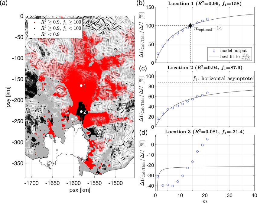
J. De Rydt et al.: Pine Island drivers of change                                                                              115

regularized Coulomb law or the plastic limit of a non-linear          The surface velocity measurements used in this study
viscous power law provides a better fit between modelled and       were taken from the MEaSUREs database (Mouginot et al.,
observed changes in surface velocity along the central flow        2019a, b). For 1996, synthetic-aperture radar data from the
line of PIG compared to a commonly used Weertman law               ERS-1 and ERS-2 missions were processed using interfer-
with a cubic dependency of the sliding velocity on the basal       ometry techniques and combined into a mosaic with an ef-
shear stress. Motivated by the above considerations, we ex-        fective timestamp of 1 January 1996. The MEaSUREs ve-
plore new ways to derive spatially variable constraints on the     locities for 2016 were based on feature tracking of Landsat 8
form of the sliding law and thereby provide the first compre-      imagery with an effective timestamp of 1 January 2016. The
hensive, spatially distributed map of basal rheology beneath       change in surface speed between the two years is shown in
PIG.                                                               Fig. 1b, and we refer to, for example, Rignot et al. (2014) and
   The remainder of this paper is organized as follows. In         Gardner et al. (2018) for a more comprehensive description
Sect. 2.1 we introduce the observational datasets used to          of these observations.
constrain and validate the ice flow model. Additional de-             To obtain an accurate estimate of the ice thickness distri-
tails about our data processing methods are provided in Ap-        bution of PIG in 1996, we compiled a time series of sur-
pendix A. Section 2.2 outlines the experimental design and         face height changes from a comprehensive set of overlap-
provides a summary of the main model components. Fur-              ping satellite altimeter data between 1996 and 2016. The
ther technical details about the model set-up and a discussion     integrated altimeter trend over the 20-year time interval,
about the sensitivity of our results to numerical model details    shown in Fig. 1c, was subtracted from the recent Bed-
are provided in Appendix B and Appendix D respectively.            Machine Antarctica reference thickness (Morlighem et al.,
Results and an accompanying discussion of all experiments          2020). As satellite altimeters are very precise instruments ca-
are provided in Sect. 3.1–3.3. Final conclusions are formu-        pable of detecting small changes in surface elevation, our ap-
lated in Sect. 4.                                                  proach is more robust compared to thickness estimates based
                                                                   on a snapshot digital elevation model, such as the ERS-1-
                                                                   derived product (Bamber and Bindschadler, 1997), which
2     Data and methods                                             has poor vertical accuracy. The BedMachine Antarctica ref-
                                                                   erence thickness is based on the high-resolution Reference
The first aim of this study is to simulate the dynamic response    Elevation Model of Antarctica (REMA; Howat et al., 2019),
of PIG to a series of well-defined geometric perturbations         tied to CryoSat-2 data, and an improved estimate of bedrock
over the period 1996 to 2016 and compare model output to           topography using mass conservation methods. The nominal
observed changes in surface speed over the same time period.       date of the BedMachine geometry corresponds to the date
As detailed in Sect. 1, geometric perturbations are considered     stamp of the REMA elevation model, which is spatially vari-
to be observed changes in the calving front position and ob-       able but largely between 2014 and 2018 for PIG. We denote
served changes in ice thickness of the ice shelf and grounded      the 1996 and BedMachine Antarctica ice thickness estimates
ice. We are primarily interested in the relative contribution      as H96 and H16 respectively, where H96 = H16 − 1H , with
of each perturbation to the observed speed-up of PIG be-           1H the integrated altimeter trend. Estimates of 1H were
tween 1996 and 2016. Each contribution can be                      based on a combination of existing Centre for Polar Obser-
                                                  characterized
by a relative change in velocity, Upert − U96 / (U16 − U96 ),      vation and Modelling (CPOM) measurements of surface el-
where U96 and U16 were obtained from model optimization            evation changes for areas upstream of the 2016 grounding
experiments, as described in Sect. 2.2.1, and velocities of the    line (Shepherd et al., 2016) and newly analysed data for the
perturbed states (Upert ) were obtained from a series of diag-     floating ice shelf. A detailed description of our methods and
nostic model calculations, as described in Sect. 2.2.2. First,     a map of the data coverage for 1H can be found in Ap-
the data sources required for each of these experiments are        pendix A and Fig. A1 respectively.
listed.                                                               The grounding line location for H16 (blue line in Fig. 1b–
                                                                   c) corresponds to the DInSAR-derived grounding line in
2.1    Observed changes of Pine Island Glacier between             2011 from Rignot et al. (2014), since this is included as a
       1996 and 2016                                               constraint in the generation of the BedMachine Antarctica
                                                                   bed topography (Morlighem et al., 2020). The grounding line
Our study area and model domain encompasses the                    for H96 = H16 − 1H approximately follows the 1992–1996
135 000 km2 grounded catchment (Rignot et al., 2011) and           DInSAR estimates (Rignot et al., 2014), as shown in Fig. A1.
seaward-floating extension of PIG in West Antarctica, as de-       To further improve the agreement between the model and
picted in Fig. 1a. To investigate the physical processes that      DInSAR grounding line in 1996, some localized adjustments
forced the contemporary speed-up of the glacier and its in-        less than 150 m were made to the bed topography. The final
crease in grounding line flux between the years 1996 and           grounding line location for H96 is depicted in Fig. 1a–c.
2016, we needed detailed observations of the surface veloc-           Alongside the above-listed observed changes in flow dy-
ity, ice thickness, and calving front position for both years.     namics and ice thickness, the calving front of PIG retreated

https://doi.org/10.5194/tc-15-113-2021                                                     The Cryosphere, 15, 113–132, 2021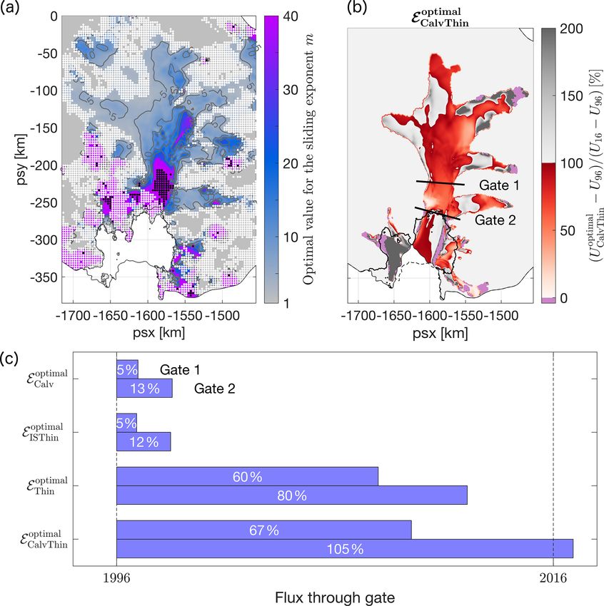
116                                                                                    J. De Rydt et al.: Pine Island drivers of change

Figure 1. Pine Island Glacier (PIG) and its location in West Antarctica. (a) Surface speed of PIG in 1996 in m yr−1 , as reported by the
MEaSUREs programme (Mouginot et al., 2019a). Solid black outlines delineate the extent of the PIG catchment (Rignot et al., 2011) and
1996 grounding line position (Rignot et al., 2014). The white line along the central flow line indicates the location of the transect in Fig. 2.
The dashed rectangle corresponds to the extent of panels (b) and (c). (b) Observed increase in surface speed (Mouginot et al. (2019a), colours
and contours in m yr−1 and loss of ice shelf extent (grey shaded area) between 1996 and 2016. The blue line indicates the 2011 grounding
line (Rignot et al., 2014). (c) Total change in ice thickness between 1996 and 2016 (1H in m), based on a combination of CPOM data
(Shepherd et al., 2016) for the grounded ice and newly analysed data for the ice shelf (Appendix A). The zero contour is shown in black;
other contours in grey are spaced at 20 m intervals.

by up to 30 km between 1996 and 2016 during a succession                  the earliest examples) to minimize the misfit between mod-
of large-scale calving events; see, for example, Arndt et al.             elled and observed surface velocities through the optimiza-
(2018). We traced the calving front positions in 1996 and                 tion of uncertain physical parameters. The optimization ca-
2016 from cloud-free Landsat 5 and Landsat 8 panchromatic                 pabilities of Úa (further details are provided in Appendix B)
band images with timestamps of 18 February 1997 and 25                    were used to optimize the uncertain spatial distribution of the
December 2016 respectively. Both outlines are included in                 rate factor, A, and basal slipperiness, C. These physical pa-
Fig. 1b–c, and the ice shelf area that was lost between 1996              rameters define the constitutive model and the relationship
and 2016 is shaded in grey.                                               between basal shear stress τ b and basal sliding velocity U b
                                                                          respectively:
2.2     Experimental design
                                                                            ˙ = AτEn−1 τ ,                                                 (2)
                                                                                                1
2.2.1    Optimization experiments                                         τ b = C −1/m kU b k   m −1   U b.                                 (3)

To obtain an optimal model configuration for the state of                 Glen’s law, Eq. (2), relates the strain rates ˙ to the deviatoric
PIG in 1996, we explicitly solved the stress balance by as-               stress tensor τ . A creep exponent n = 3 was used throughout
similating the estimated ice thickness (H96 ), measured calv-             this study. Equation (3) is known as a Weertman sliding law
ing front position, and measured surface velocities in the                (Weertman, 1957) and describes a linear viscous, non-linear
shallow ice stream model Úa (Gudmundsson et al., 2012;                    viscous, or close-to-plastic bed rheology for m = 1, m > 1,
Gudmundsson, 2020). An analogous routine was applied for                  and m  1 respectively. Throughout this study, a range of
2016. This “data assimilation” or “optimization” step is com-             values for m are considered, as specified below. For each m
monly adopted in glaciology (see MacAyeal, 1992, for one of               we performed a new inversion for A and C; example results

The Cryosphere, 15, 113–132, 2021                                                                https://doi.org/10.5194/tc-15-113-2021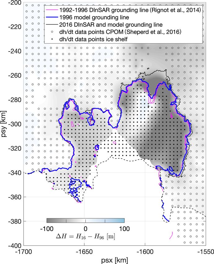
J. De Rydt et al.: Pine Island drivers of change                                                                             117

for m = 3 are provided in Appendix B. The outcome of the                m
                                                                    – ECalvThin . Combined changes in calving front position
optimization step is an estimate for A and C that best fits the               m ) and thinning (as in E m ) were prescribed.
                                                                      (as in ECalv                     Thin
stress balance in Eq. (1) for given observations of geome-            Corresponding velocity changes will be denoted by
try and surface velocity, associated measurement errors, and          1UCalvThin = UCalvThin − U96 .
assumptions about the prior values of A and C. Solutions
                                                                  A schematic overview of the experiments is provided in
for A and C are not generally unique but rather depend on                           m
                                                                  Fig. 2. While ECalv   allows us to assess the instantaneous
the choice of optimization scheme and several poorly con-
                                                                  impact of calving between 1996 and 2016, the experiments
strained optimization parameters. Further details about the         m
                                                                  EISThin simulate the instantaneous response to total changes
optimization scheme used and a discussion about the robust-
                                                                  in ice shelf thickness between 1996 and 2016. The separate
ness of our results with respect to uncertain optimization pa-
                                                                  perturbations make it possible to disentangle changes in ice
rameters are provided in Appendix B and D.
                                                                  shelf buttressing caused by each process, and hence their rel-
2.2.2   Geometric perturbation experiments                        ative importance for driving the transient evolution of the
                                                                  flow. However, both experiments ignore the time-dependent,
The optimal model configuration in 1996 was subsequently          dynamic response of the upstream grounded ice and the as-
used as the reference state for a series of numerical perturba-   sociated loss of basal traction due to grounding line move-
tion experiments, aimed at simulating the impact of observed      ment. Dynamic thinning of grounded ice, as well as migra-
changes in geometry on the flow of PIG. For each perturba-        tion of the grounding line, is included in the experiments
                                                                    m , which allows us to determine the full dynamic re-
                                                                  EThin
tion, the modified force balance (Eq. 1) and corresponding
perturbed velocities were diagnosed within Úa. The rate fac-      sponse to changes in ice thickness. Finally, the experiments
                                                                    m
                                                                  ECalvThin combine both calving and ice thinning, and thereby
tor and basal slipperiness were kept fixed to their 1996 val-
ues, although the basal traction was reduced to zero and slip-    accounts for all geometric perturbations.
periness values became irrelevant in areas that ungrounded
                                                                  2.2.3   Estimates of changes in A and C
due to ice thinning. Experiments will be referred to as E∗m ,
with a variable subscript to indicate the type of perturbation    Later on we show that geometric perturbations alone are
and a superscript to specify the value of the sliding exponent    not able to fully reproduce the observed patterns of speed-
m.                                                                up across the PIG catchment. It is conceivable that, along
      m . Changes in the calving front location were pre-         with the evolving geometry, variations in ice and basal
  – ECalv
                                                                  properties have contributed to the changes in flow between
    scribed to reflect the loss of ice shelf between 1996 and
                                                                  1996 and 2016. Indeed, feedback mechanisms are likely
    2016 (see Fig. 1b–c). All model grid elements down-
                                                                  to cause an important interdependence between geometry-
    stream of the 2016 calving front (grey shaded area in
                                                                  induced changes in ice flow, shear softening, and/or changes
    Fig. 1b) were deactivated, whilst elements upstream of
                                                                  in basal shear stress. Reliable observations of changes in rhe-
    the 2016 calving front remained fixed to avoid numeri-
                                                                  ology and basal properties are not available, but numerical
    cal interpolation errors. All other model variables were
                                                                  optimization simulations can provide valuable insights into
    kept fixed. The difference between the 1996 surface ve-
                                                                  their evolution. We used the inverse method as described in
    locity and the perturbed velocity will be denoted by
                                                                  Sect. 2.2.1 and Appendix B to estimate necessary bounds on
    1UCalv = UCalv − U96 .
                                                                  the magnitude and spatial distribution of changes in A and
      m
  – EISThin . Changes in ice shelf thickness were prescribed,     C that are required, beside the geometrical changes already
    corresponding to observed thinning of the ice shelf be-       applied, to produce the speed-up of PIG between 1996 and
    tween 1996 and 2016 (Fig. 1c). Note that the calv-            2016. Changes in A and C are treated separately.
    ing front and grounding line location did not change            – EAm . The aim of these experiments is to determine pos-
    in this experiment, which is similar to previous stud-            sible changes in the rate factor between 1996 (A96 ) and
    ies by, for example, Reese et al. (2018) and Gudmunds-            2016 (A16 ). A96 was previously obtained in part 1 (op-
    son et al. (2019). The instantaneous change in surface            timization step) of the experimental design. To estimate
    velocity due to ice shelf thinning will be denoted by             A16 , an inverse optimization problem was solved for the
    1UISThin = UISThin − U96 .                                        2016 PIG geometry (H16 ) and velocities (U16 ), but us-
      m . Observed changes in both the floating and                   ing a cost function that was minimized with respect to
  – EThin
                                                                      A only. The slipperiness C was kept fixed to its 1996
    grounded parts of PIG were prescribed. This caused the
                                                                      solution.
    grounding line to move from its 1996 position (black
    line in Fig. 1b–c) to the 2016 position (blue line in           – ECm . These experiments are analogous to EAm , but the cost
    Fig. 1b–c). Velocity changes caused by thinning of the            function in the inverse problem was optimized with re-
    floating and grounded ice will be denoted by 1UThin =             spect to C only, whereas the rate factor A was kept fixed
    UThin − U96 .                                                     to its 1996 solution.

https://doi.org/10.5194/tc-15-113-2021                                                    The Cryosphere, 15, 113–132, 2021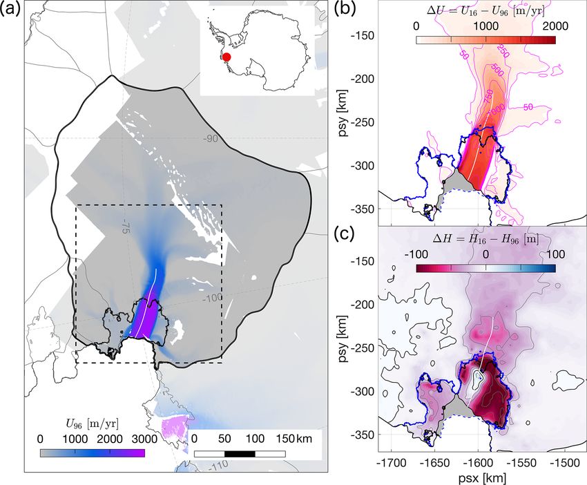
118                                                                                   J. De Rydt et al.: Pine Island drivers of change

Figure 2. Overview of changes along the Pine Island Glacier centreline from (a) year 1996 to (b) year 2016. Increased ice flow is driven
by a combination of calving, ice shelf thinning, and dynamic thinning with movement of the grounding line, as well as changes in basal
sliding and ice rheology. Transects of the geometry are based on observations along the flow line indicated in Fig. 1; black dots indicate the
respective grounding line positions in both years. Crevasses are introduced for illustration purposes only and do not strictly correspond to
observed features. The importance of each “driver of change” was investigated in a series of numerical perturbation experiments, denoted by
E∗m in panel (b), with m indicating the sliding exponent and ∗ the respective experiment described in Sect. 2.2.

3     Results and discussion                                             it accounts for up to 50 % of the observed speed-up between
                                                                         1996 and 2016 (Fig. 3a). A smaller dynamical impact is also
3.1    Ice dynamic response to changes in geometry                       felt upstream of the grounding line, caused by the calving-
       between 1996 and 2016                                             induced reduction in ice shelf buttressing and mechanical
                                                                         coupling between the floating and grounded ice. Along the
                                                                         fast-flowing central trunk of PIG, calving typically accounts
We present results for the first set of perturbation experi-             for less than 10 % of the observed speed-up, with little or
ments, which simulate the impact of observed changes in                  no effect on the dynamics of the upstream tributaries. Our
geometry on the flow of PIG. As detailed in Sect. 2.2.2, per-            results are consistent with earlier work by Schmeltz et al.
turbations are split between four separate cases: (1) calving            (2002), in particular their calving scenario “part 2”. The only
   3 ); (2) thinning of the ice shelf (E 3
(ECalv                                    ISThin ); (3) thinning         area with negative relative changes in our simulation is the
of the ice shelf and grounded ice (EThin 3 ), which includes
                                                                         western shear margin of the ice shelf, where modelled and
associated movement of the grounding line and changes in                 observed changes in flow speed have the opposite sign. Ex-
basal traction; and (4) the combined impact of all the above             tensive damage, a process that is not captured by this ex-
   3
(ECalvThin ). We did not previously specify the value of the             periment, has caused this margin to migrate, and significant
sliding exponent; however, here we set m = 3, which is a                 interannual variations in flow speed have been reported by
commonly adopted value in ice flow modelling and describes               Christianson et al. (2016). Figure 3e shows that calving ac-
a non-linear viscous (or Weertman) bed rheology. Results for             counts for 2 and 13 % of the observed flux changes through
different values of m will be explored in Sect. 3.3.                     Gate 1 and 2 respectively, which confirms the minor instan-
   Results for the relative change in surface speed,                    taneous changes to the flow upstream of the grounding line.
 Upert − U96 / (U16 − U96 ), for each of the above perturba-                 Thinning of the ice shelf as simulated in experiment
tions are presented in Fig. 3a–d. In addition to spatial maps              3
                                                                         EISThin induces a flow response that is similar to calving, as
of relative velocity changes, we present flux calculations for           shown in Fig. 3b, and indicates that calving and ice shelf
two gates perpendicular to the flow within the central part of           thinning have caused a comparable perturbation in the but-
PIG, as displayed in Fig. 3a. Gate 1 is situated about 50 km             tressing forces. The largest percentage changes are found on
upstream of the 2016 grounding line and captures the inland              the ice shelf and are typically less than 25 %, while the rel-
propagation of changes in ice flow. Gate 2 approximately co-             ative flux changes through Gate 1 and 2 are identical to the
incides with the 2016 grounding line position and captures               calving experiment (Fig. 3e). Ice shelf thinning is generally
changes in grounding line flux, which is a direct measure for            accepted to be the main driver of ongoing mass loss of PIG,
PIG’s increasing contribution to sea level rise and an impor-            and patterns of ice shelf thinning elsewhere in Antarctica are
tant indicator of change.                                                strongly correlated to observed changes in grounding line
                             3
   Calving as simulated in ECalv causes changes in flow speed            flux (Reese et al., 2018; Gudmundsson et al., 2019). How-
that are predominantly restricted to the outer ice shelf, where

The Cryosphere, 15, 113–132, 2021                                                               https://doi.org/10.5194/tc-15-113-2021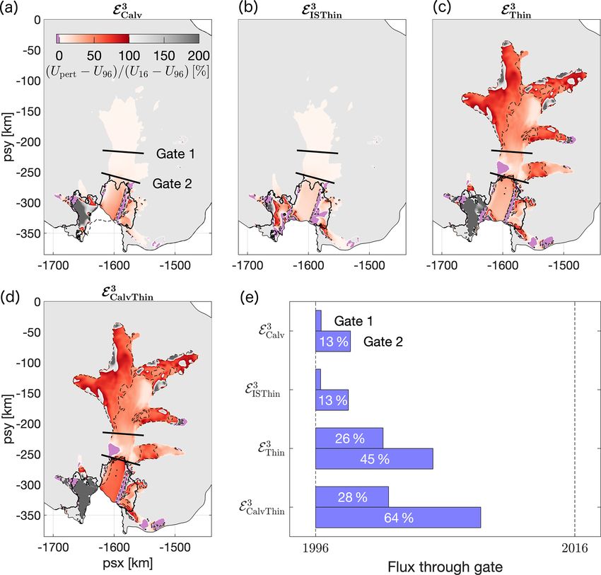
J. De Rydt et al.: Pine Island drivers of change                                                                                             119

Figure 3. Modelled changes in surface speed compared to 1996 for prescribed perturbations of the Pine Island Glacier geometry. (a) Retreat
of the calving front. (b) Thinning of the ice shelf. (c) Thinning of the ice shelf and grounded ice, including grounding line retreat. (d) Calving
and thinning combined. For each perturbation, the modelled change in speed (Upert −U96 ) is expressed as a percentage of the observed speed-
up between 1996 and 2016 (U16 − U96 ). Dashed black lines correspond to the 50 % contour. Panel (e) shows the percentage of the observed
flux changes through Gate 1 and 2 that can be explained by the respective perturbations. The simulated impact of calving and thinning in
               3
experiment ECalvThin    only represents 28 and 64 % of the measured flux changes respectively. Possible explanations for the unaccounted-for
increase in flow speed are provided in Sect. 3.2 and 3.3 .

ever, the force perturbations that result from ice shelf thin-             floating ice shelf and upstream grounded ice. This perturba-
ning alone, in particular the instantaneous reduction in back              tion incorporates the observed recession of the PIG ground-
forces τ IS , are not sufficient to reproduce the magnitude of             ing line between 1996 and 2016. The combined reduction in
observed changes in upstream flow, consistent with previous                ice shelf buttressing, loss of basal friction due to grounding
studies (Seroussi et al., 2014; Joughin et al., 2010, 2019).               line retreat, and changes in driving stress caused a significant
                        3
Indeed, experiment EISThin      demonstrates that the direct and           and far-reaching impact on the flow, as displayed in Fig. 3c.
instantaneous contribution of ice shelf thinning to observed               Modelled changes on the ice shelf are consistent with and
changes in grounding line flux is less than 25 %. Instead,                                             3
                                                                           similar in amplitude to EISThin  . Upstream of the grounding
time-evolving changes in geometry and mass redistribution                  line, modelled changes relative to observations are between
upstream of the grounding line, which may cause grounding                  25 and 50 % along the central trunk and up to 100 % along
line retreat and associated loss of basal traction, play a signif-         the tributaries. In addition, results demonstrate that glacier-
icant role in increasing the dynamic response of the glacier.              wide changes in ice thickness account for 26 and 45 % of the
These dynamic changes, caused indirectly by changes in the                 observed changes in ice flux through Gate 1 and 2 respec-
calving front position and ice shelf thinning, were not cap-               tively (Fig. 3e).
tured by the experiments ECalv3         3
                                  and EISThin but are considered                                                        3
                                                                              In the final perturbation experiment, ECalvThin  , the com-
                  3
in experiment EThin .                                                      bined effect of calving and changes in ice thickness was sim-
   In experiment EThin3     we prescribed the time-integrated              ulated. Modelled versus observed changes in surface speed
change in ice thickness between 1996 and 2016 for both the                 are shown in Fig. 3d. The spatial pattern is consistent with

https://doi.org/10.5194/tc-15-113-2021                                                                The Cryosphere, 15, 113–132, 2021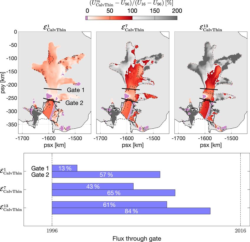
120                                                                             J. De Rydt et al.: Pine Island drivers of change

previous experiments, and the amplitude of the response is           explanation for the discrepancy between simulated and ob-
approximately equal to the added response of experiments             served changes in the surface speed of PIG in the geometric
  3
ECalv       3 , i.e. 1U
       and EThin                                                                    3
                                                                     experiment ECalvThin  . Experiment EA3 assumes that, in addi-
                         CalvThin ≈ 1UCalv +1UThin . The cor-
responding percentage changes in ice flux through Gate 1 and         tion to changes in geometry, temporal variations in A alone
2 are 28 and 64 % respectively, whereas modelled changes             are able to account for the significant increase in flux that
in flow across the actual grounding line account for about           was unaccounted for in previous experiments. Alternatively,
75 % of the observed increase in flux between the years              EC3 assumes that, in addition to changes in geometry, tempo-
1996 and 2016. Although this experiment prescribes all ob-           ral variations in C alone are able to resolve the discrepancy
served changes in PIG geometry over the observational pe-            in Sect. 3.1 between the modelled and observed speed-up.
riod, model simulations are unable to capture a significant          In line with previous experiments we assume a Weertman
percentage of the observed speed-up. This is most noticeable         sliding law with m = 3. The results for both experiments are
along the fast-flowing central trunk upstream of the ground-         summarized in Fig. 4.
ing line, whereas discrepancies decrease along the slow-                Changes in A (Fig. 4a) needed to fully reproduce the
flowing tributaries in the high catchment. We also note that,        speed-up of PIG between the years 1996 and 2016 are spa-
in one area between Gate 1 and 2, modelled and observed              tially coherent and predominantly positive. This suggests a
changes in surface speed have opposite signs.                        reduction in ice viscosity between 1996 and 2016, as a result
    Although it is not unexpected to find differences between        of localized heating, enhanced damage within the ice col-
diagnostic model output and observations, the consistently           umn, or changes in anisotropy. The largest changes are found
suppressed response of the model to realistic perturbations in       in distinct geographical areas: a localized increase within the
ice geometry is indicative of a structural shortcoming within        shear margins of the ice shelf and a more widespread increase
our experimental design. Indeed, results show that, for a non-       along the slower-moving flanks (magenta contours in Fig. 4a
linear viscous bed rheology described by a Weertman sliding          indicate surface speed in 2016) of the main glacier and west-
law with constant sliding coefficient m = 3, changes in ice          ernmost tributary, about 20 km upstream of the 2016 ground-
geometry alone cannot account for the complex and spatially          ing line. Changes within the ice shelf shear margins are con-
variable pattern of speed-up over the observational period,          sistent with their increasingly complex and damaged mor-
i.e. U16 − U96 6 = 1UCalvThin . In the remainder of this study,      phology, as is apparent from satellite images (Alley et al.,
two possible hypotheses are analysed that enable the gap to          2019). Weakening of the ice in these areas is sufficient to ac-
be closed between geometry-induced changes in ice flow and           count for the remaining 50 % of observed changes in ice shelf
the observed speed-up of PIG. The first hypothesis, which is         speed-up that could not previously be reproduced by calv-
considered in Sect. 3.2, assumes that bed deformation can                                                                3
                                                                     ing and ice shelf thinning alone (experiment ECalThin     ). Pro-
indeed be described by a non-linear viscous power law with           jected changes in A along the flanks of the upstream glacier,
m = 3, but further temporal variations in ice viscosity and/or       on the other hand, are more ambiguous. Values in excess
basal slipperiness are required in addition to changes in ge-        of 10−7 yr−1 kPa−3 correspond to an equivalent increase in
ometry: U16 −U96 = 1UCalvThin +1UA +1UC . The second,                “ice” temperature by up to 40 ◦ C. This is nonphysical unless
alternative hypotheses, discussed in Sect. 3.3, assumes that         (part of) the change is attributed to damage or evolution of
internal properties of the ice and bed have not significantly        the ice fabric. Based on our analysis of Sentinel and Land-
changed between the years 1996 and 2016, i.e. 1UA ≈ 0 and            sat satellite images, there is no obvious indication of recent
1UC ≈ 0, but a different physical description of the basal           changes in the surface morphology in these areas. Either sig-
rheology is required instead.                                        nificant and widespread changes in the thermal and mechan-
                                                                     ical properties have occurred beneath the surface or the ob-
3.2   Changes in the rate factor and basal slipperiness              served speed-up and thinning in these areas, as previously
      between 1996 and 2016                                          reported by Bamber and Dawson (2020), cannot be convinc-
                                                                     ingly attributed to changes in the rate factor.
In transient model simulations of large ice masses such as              Alternatively, temporal changes in C can be invoked to re-
Antarctica’s glaciers and ice streams, it is common to assume        produce the discrepancies between modelled and observed
that the advection of A with the ice, or changes due to tem-         changes in surface speed between the years 1996 and 2016.
perature variations and fracture as well as changes in basal         Results presented in Fig. 4b suggest that a complex and
slipperiness C, exerts a second-order control on changes in          widespread pattern of changes in the slipperiness is required
ice flow. As such, temporal variability in A and C is often          across an extensive portion of PIG’s central basin and its up-
ignored, based on the assumption that these changes are suf-         per catchment. Despite the complex and poorly understood
ficiently slow and do not significantly affect the flow on typi-     relationship between C and quantifiable physical properties
cal decadal to centennial timescales under consideration. The        of the ice–bed interface, it is difficult to understand how any
aim of experiments EA3 and EC3 , as outlined in Sect. 2.2.3, is to   single process or combination of physical processes could be
establish whether this is a valid assumption, or whether pre-        responsible for the large and widespread changes in C over a
viously ignored changes in A and/or C can provide a realistic        time period of 2 decades. Further information, such as a time

The Cryosphere, 15, 113–132, 2021                                                         https://doi.org/10.5194/tc-15-113-2021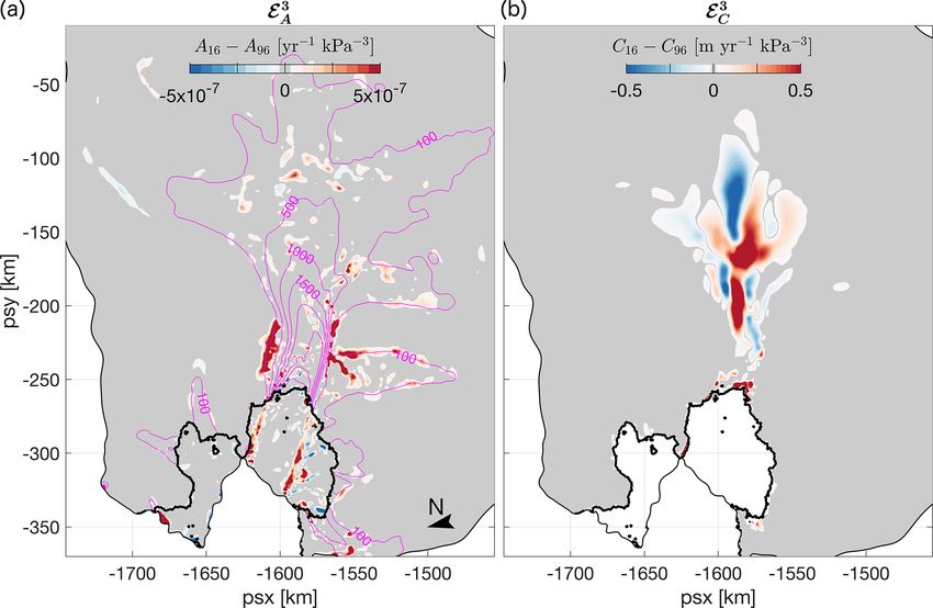
J. De Rydt et al.: Pine Island drivers of change 121
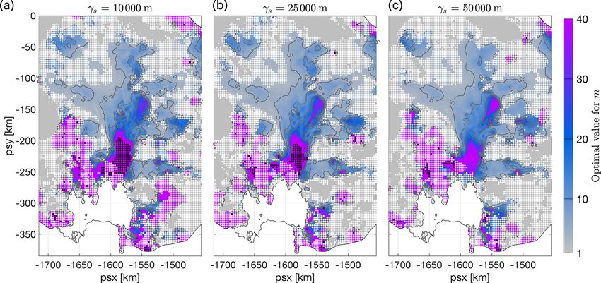
Figure 4. (a) Results for the EA3 experiment: changes in the rate factor A required to fully reproduce observed changes in surface speed of
the ice shelf and grounded ice between the years 1996 and 2016. The sliding exponent m = 3 and basal slipperiness C were kept fixed for
grounded areas. Magenta contours (in m yr−1 ) correspond to the surface speed in 2016. (b) Results for the EC3 experiment: changes in the
basal slipperiness C required to reproduce the observed increase in surface speed of the grounded ice between 1996 and 2016. The rate factor
A is assumed constant between 1996 and 2016.
series of maps similar to Fig. 4b, can potentially be used to law rheology is particularly suitable for the description of
test the robustness of this result and provide further insights hard-bedded sliding without cavitation (Weertman, 1957),
into the physical processes that could control such changes. but missing processes such as variations in effective pressure
This is the subject of future research. or the deformation of a subglacial till layer with a maximum
We note that, in the EC3 experiment, velocities on the float- shear (yield) stress could be important limitations. Some ev-
ing ice shelf were largely unaffected by changes in C and idence has been provided for plastic bed properties under-
remained significantly slower than observations (not shown). neath ice streams either from observations (Tulaczyk et al.,
In contrast, changes in the rate factor were able to fully 2000; Minchew et al., 2016) or from laboratory experiments
account for the speed-up of the ice shelf. On the other (Zoet and Iverson, 2020). Most recently, Gillet-Chaulet et al.
hand, large variations in A were needed to reproduce the (2016), Brondex et al. (2019), and Joughin et al. (2019) used
changes in ice dynamics along the slow-moving flanks of numerical simulations to show that different sliding laws can
PIG (Fig. 4a), whereas only small changes in C less than cause a distinctly different dynamical response of PIG to
10−3 yr−1 kPa−3 m were required to explain this behaviour. changes in geometry, and observed changes in surface ve-
It is therefore conceivable that, in addition to PIG’s evolv- locity were best reproduced for sliding exponents m
1 or
ing geometry, an intricate combination of changes in both using a hybrid law that combines power law with Coulomb
the rate factor and basal slipperiness are required to repro- sliding. Although the results are compatible with a plastic
duce the glacier’s complex and spatially diverse patterns of bed underlying the central trunk of PIG, no constraints on
speed-up over the last 2 decades. It is however not straight- the spatial variability in basal rheology were derived.
forward to disentangle these processes in the current mod- In order to quantify how different values of the sliding
elling framework. exponent affect the sensitivity of PIG to changes in geom-
etry across the catchment, we repeated perturbation experi-
m
ments ECalvThin for a range of sliding-law exponents, from
3.3 Evidence for a heterogeneous bed rheology
m = 1 to m = 21 at increments of 2. Results for m = 1, 7,
The relationship between changes in geometry and the dy- and 13 are shown in Fig. 5. A linear rheology induces a sim-
namic response of a glacier crucially depends on the me- ulated response to calving and thinning that accounts for less
chanical properties of the underlying bed and subglacial hy- than 50 % of the observed changes everywhere. For m = 7,
drology. So far, we have assumed that basal sliding can be relative changes in flow speed exceed 100 % along signifi-
represented by a non-linear viscous power law with spa- cant portions of the slower-flowing tributaries. For m = 13,
tially uniform stress exponent m = 3 (see Eq. 3). A power- which effectively corresponds to a plastic rheology, the mod-
https://doi.org/10.5194/tc-15-113-2021 The Cryosphere, 15, 113–132, 2021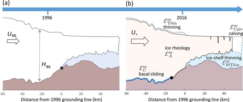
122                                                                                 J. De Rydt et al.: Pine Island drivers of change

Figure 5. Dependency of simulated-versus-observed changes in surface speed on the sliding-law exponent: (a) m = 1, (b) m = 7, and (c)
m = 13. Dashed black lines correspond to the 50 % contour. Larger values of m cause an increased response of the modelled surface speed
to geometrical changes (calving, thinning, and grounding line retreat). For m > 3, the modelled response of slow-flowing ice in the upstream
catchment exceeds observed changes by more than a factor of 2, whereas for m = 13 modelled changes of the fast-flowing central trunk are
still smaller than observed changes. (d) Changes in flux through Gate 1 and 2 as a percentage of observed changes for m = 1, 7, and 13.

elled response overshoots observations by more than 100 %               (2008) and depends on m in the following non-linear way:
in most areas, except along the main glacier, where the re-
sponse approaches 100 %. Across the model domain, a sig-                                         f1 m
                                                                        δU ≡ |TUS (m)|δS =             δS .                              (4)
nificant positive correlation exists between m and relative                                     m + f2
velocity changes, indicating a stronger dynamic response to
perturbations in geometry with increasing values of m. This             The transfer amplitude |TUS | contains complicated positive
finding is in agreement with Gillet-Chaulet et al. (2016) and           functions f1 and f2 that generally depend on the wavelength
Joughin et al. (2019); however our maps show that no single,            of the surface perturbation, geometrical factors such as the
spatially uniform value of the sliding exponent is able to pro-         local bed slope, and the basal slipperiness C. Further de-
duce a good match between model output and observations                 tails are provided in Appendix C. Despite the simplifying as-
across the entire catchment.                                            sumptions that underlie the analytical expression of |TUS | ob-
   The positive correlation between the flow response and m             tained by Gudmundsson (2008), results from our simulations
                                                                          mi
is an inherent property of the adopted physical description of          ECalvThin , mi ∈ {1, 3, · · ·, 21}, indicate that Eq. (4) is also ap-
glacier dynamics. For the shallow ice stream approximation              plicable to the more complex setting of PIG. Indeed, as ex-
with a non-linear viscous sliding law, the first-order response         plained in detail in Appendix C, we found that across a large
of the surface velocity, δU , to small perturbations in surface         portion of the PIG catchment the transfer amplitude |TUS |
elevation, δS, was previously determined by Gudmundsson                 provides a suitable model to describe the dependency of the
                                                                        relative velocity changes 1UCalvThin / (U16 − U96 ) on m. The
                                                                        parameters f1 and f2 were treated as spatially variable fields,
                                                                        and best estimates f1∗ (x) and f2∗ (x) were obtained as a solu-

The Cryosphere, 15, 113–132, 2021                                                              https://doi.org/10.5194/tc-15-113-2021
J. De Rydt et al.: Pine Island drivers of change 123
tion of the minimization problem non-linear regression was generally found to be poor, with
R 2 values smaller than 0.9 as indicated by the white dots in
m
1UCalvThin (x)
f1 (x)m Fig. 6a. As no reliable estimate for moptimal could be obtained
f1∗ (x), f2∗ (x)
= min − , for areas shaded in white or black in Fig. 6a, values were in-
f1 ,f2 m + f2 (x) U16 − U96
stead based on a nearest-neighbour interpolation.
with m ∈ {1, 3, · · ·, 21} .
It is important to reiterate that the regression method used
(5) crucially relies on non-trivial measurements of changes in
m surface velocity (U16 − U96 6 = 0) and cannot be used to re-
The non-linear dependency of 1UCalvThin / (U16 − U96 ) on m trieve information about the basal rheology of ice bodies
can then be approximated by that are presently in steady state. It should also be noted
m
1UCalvThin f ∗ (x)m that values of f1∗ (x) and f2∗ (x) were derived independently
≈ 1 ∗ . (6) for each node of the computational mesh, whereas the con-
U16 − U96 m + f2 (x)
tinuum mechanical properties of glacier flow would sug-
Using this dependency of the simulated velocity changes gest a non-zero spatial covariance hf1 (x 1 ), f1 (x 2 )i 6= 0 and
on m, one can derive an “optimal” spatial distribu- hf2 (x 1 ), f2 (x 2 )i 6 = 0. The optimal solution for m is therefore
tion of the sliding exponent, moptimal (x), such that not automatically mesh independent or robust with respect to
1UCalvThin / (U16 − U96 ) = 100 % everywhere, namely the amount of regularization in the inversion. This concern is
discussed further in Appendix D.
f2∗ (x) In order to demonstrate the improved model response to
moptimal (x) = ∗ . (7) thinning and calving for a spatially variable sliding exponent
f1 (x) − 1
moptimal (x), we performed a new inversion with moptimal (x)
By construction, the variable sliding exponent moptimal (x) and subsequently repeated the geometric perturbation exper-
enables reproducing 100 % of the observed speed-up of PIG optimal
iments E∗ . The results are presented in Fig. 6b and c.
in response to calving and ice thickness changes. The re- Compared to spatially uniform values of m (Fig. 3d and
sults, depicted in Fig. 6a, indicate that plastic bed conditions Fig. 5), a spatially variable basal rheology generally im-
(m
1) prevail across most of the fast-flowing central val- proves the fit between observed changes in flow and the
ley and parts of the upstream tributaries. Values generally modelled response across the entire basin. Based on the flux
increase towards the grounding line, whilst linear or weakly changes through Gate 1 and 2, we find that (1) calving and
non-linear bed conditions are consistently found in the slow- ice thickness changes in combination with a spatially vari-
flowing inter-tributary areas. This finding is compatible with able, predominantly plastic bed rheology account for 67 and
the presence of a weak, water-saturated till beneath fast- 105 % of flux changes through Gate 1 and 2 respectively,
flowing areas of PIG and a hard bedrock or consolidated till compared to 28 and 64 % for a uniform non-linear viscous
between tributaries (Joughin et al., 2009). The transition to sliding law with exponent m = 3; that (2) calving and ice
lower exponents in areas with slower flow (< 600 m a−1 ) is shelf thinning caused an almost identical response in ice dy-
also consistent with results based on a Coulomb-limited slid- namics upstream of the grounding line; and that (3) dynamic
ing law, which produces Coulomb plastic behaviour at speeds thinning and grounding line movement account for most of
> 300 m a−1 and weakly non-linear viscous sliding at slower the flux changes between the years 1996 and 2016. The re-
speeds (Joughin et al., 2019). maining mismatch between the observed and modelled re-
Two interesting properties of the regression model in sponse in Fig. 6b can, at least in part, be attributed to un-
Eq. (4) are worth noting. Firstly, for m → ∞, the function certainties in moptimal (x). This is of particular relevance in
|TUS | approaches a horizontal asymptote with limit equal to the vicinity of the grounding line and for parts of the central
f1 . As a consequence, the associated solution for moptimal trunk, where the non-linear regression method in Eq. (4) did
diverges to ∞ for locations x where f1∗ (x) = 100 and be- not provide a reliable or finite estimate for moptimal . Previ-
comes negative where f1∗ (x) < 100. In these areas, indicated ous studies, for example by Gillet-Chaulet et al. (2016) and
by black dots in Fig. 6a, no non-negative, finite value of m ex- Joughin et al. (2019), have demonstrated a better agreement
ists such that 1UCalvThin (x)/ (U16 − U96 ) = 100 %, and con- between modelled and observed speed-up using Coulomb-
ventional Weertman sliding is unable to fully reproduce the limited sliding laws, such as those proposed by Budd et al.
observed flow changes in response to thickness changes and (1984), Schoof (2006), and Tsai et al. (2015). Our results are
calving. Either a different form of the sliding law is required consistent with these earlier studies and suggest that power-
or additional changes in the rate factor A and/or basal slip- law sliding does not adequately capture the physical relation-
periness C are needed. These findings are the subject of a ship between basal shear stress and sliding in the vicinity of
forthcoming study. Our second observation concerns loca- the grounding line.
tions where U16 or U96 contains significant measurement un-
certainties, or where no discernible changes in the surface ve-
locity were measured, i.e. U16 − U96 ≈ 0. In these areas, the
https://doi.org/10.5194/tc-15-113-2021 The Cryosphere, 15, 113–132, 2021124 J. De Rydt et al.: Pine Island drivers of change
Figure 6. (a) Optimal values of the sliding exponent, required to ensure close agreement between modelled and observed changes in flow ve-
locity of Pine Island Glacier between the years 1996 and 2016. White and black dots mark areas where such an agreement cannot be achieved
mi
for different reasons: white dots indicate a poor fit between the transfer function |TUS | and 1UCalvThin / (U16 − U96 ) , mi ∈ {1, 3, · · ·, 21},
with R 2 < 0.9; black dots indicate areas where a positive, finite solution for moptimal in Eq. (7) does not exist and non-linear viscous sliding
cannot reproduce observed changes in surface flow. (b) Same as Fig. 3d but for optimal values of the sliding-law exponent in panel (a).
(c) Same as Fig. 3e but for optimal values of the sliding-law exponent in panel (a).
4 Conclusions grounding line, whereas the remaining 36 % could be at-
tributed to large and widespread changes in ice viscosity (in-
Based on the most comprehensive observations of ice shelf cluding damage) and/or changes in basal slipperiness. Under
and grounded ice thickness changes to date, and a suite of the alternative assumption that ice viscosity and basal slip-
diagnostic model experiments with the contemporary flow periness did not change considerably over the last 2 decades,
model Úa, we have analysed the relative importance of ice we found that the recent increase in flow speed of Pine Island
shelf thinning, calving, and grounding line retreat for the Glacier is only compatible with observed patterns of thinning
speed-up of Pine Island Glacier over the period 1996 to 2016. if a heterogeneous, predominantly plastic bed underlies large
The detailed comparison between simulated and observed parts of the central glacier and its upstream tributaries, con-
changes in flow speed has provided insights into the ability of sistent with the earlier literature.
a modern-day ice flow model to reproduce dynamic changes
in response to prescribed geometric perturbations. Signifi-
cant discrepancies between observed and modelled changes
in flow were found and addressed either by allowing changes
in ice viscosity and basal slipperiness or by varying the me-
chanical properties of the ice–bed interface. For non-linear
viscous sliding at the bed, geometric perturbations could only
account for 64 % of the observed flux increases close to the
The Cryosphere, 15, 113–132, 2021 https://doi.org/10.5194/tc-15-113-2021J. De Rydt et al.: Pine Island drivers of change 125
Appendix A: Observations of Pine Island Ice Shelf
thickness changes between 1996 and 2016
We derived a new ice shelf height time series from measure-
ments acquired by four overlapping ESA satellite radar al-
timetry (RA) missions: ERS-1 (1991–1996), ERS-2 (1995–
2003), Envisat (2002–2012), and CryoSat-2 (2010–present).
For this study, we constructed a record of ice shelf height
spanning 20 years (1996–2016), with a temporal sampling of
3 months. We integrated all measurements along the satellite
ground tracks and gridded the solution on a 3 km by 3 km
grid.
Our adopted processing steps for RA data are a modi-
fication/improvement from Paolo et al. (2016) and Nilsson
et al. (2016). Specifically for CryoSat-2, we retracked ESA’s
SARIn L1B product over the Antarctic ice shelves using
the approach by Nilsson et al. (2016), corrected for a 60 m
range offset for data with surface types “land” or “closed
sea”, and removed points with anomalous backscatter val-
ues (> 30 dB). We estimated heights with a modified (from
McMillan et al., 2014) surface-fit approach, with a variable
rather than constant search radius to account for the RA
heterogeneous spatial distribution, calculating mean values Figure A1. Ice thickness changes (1H ) between 1996 and 2016,
along the satellite reference tracks; we removed height es- based on a comprehensive analysis of satellite altimeter data. The
timates less than 2 m above the EIGEN-6C4 geoid (Chuter altimeter data coverage is represented by dots (ice shelf) and cir-
and Bamber, 2015) to account for ice shelf mask imperfec- cles (grounded ice; Shepherd et al., 2016). The final 1996 ice thick-
tions near the calving front; we applied all of the standard ness distribution was obtained by subtracting 1H from the 2016
corrections to altimeter data over ice shelves (for example, BedMachine ice thickness (Morlighem et al., 2020), as described in
removing gross outliers and residual heights with respect to Sect.2.1. The associated 1996 grounding line location (blue line)
mean topography > 15 m); we ran an iterative 3σ filter; we compares well to independent DInSAR measurements (magenta
minimized the effect of variations in backscatter (Paolo et al., line; Rignot et al., 2014).
2016); and we corrected for ocean tides (Padman et al., 2002)
and inverse barometer effects (Padman et al., 2004).
tral flow line. Here, thickness changes were obtained through
We then gridded the height data in space and time on
linear interpolation from neighbouring data. The grounding
a 3 km × 3 km × 3-month cube, for each mission indepen-
line location associated with our 1996 thickness distribution
dently. We merged the records (all four satellites) by only
was compared to independent measurements from DInSAR
accepting time series that overlapped by at least three quar-
(Rignot et al., 2014), and both agree well (Fig.A1).
ters of a year to ensure proper cross-calibration, and removed
(and subsequently interpolated) anomalous data points that
deviated from the trend by more than 5 SD. This removes Appendix B: Model configuration and optimization
data with, for example, satellite mispointing, anomalous
backscatter fluctuations, grounded-ice contamination, high The open source ice flow model Úa (Gudmundsson,
surface slopes, and geolocation errors. We fitted linear trends 2020) uses the finite-element method to solve the shal-
to the gridded product to obtain the 1H field used in our low ice stream equations, commonly referred to as SSA or
model experiments (see Sect. 2.1). We also removed a 3 km SSTREAM (Hutter, 1983; MacAyeal, 1989), on an irregu-
buffer around the ice shelf boundaries to further mitigate lar triangular mesh. The diagnostic velocity solver is based
floating–grounded mask imperfections and the limitation of on an iterative Newton–Raphson method. A fixed mesh with
geophysical corrections within the ice shelf flexural zone. 109 300 linear elements was used with a median nodal spac-
The thickness changes for the ice shelf were combined ing of 1.2 km and local mesh refinement down to 500 m in
with existing data for thickness changes over the same time areas with above-average horizontal shear, with strong gra-
period on the grounded ice (Shepherd et al., 2016). The re- dients in ice thickness, and within a 10 km buffer around
sulting dataset for 1H , as used in the experiments described the grounding line. The mesh was generated using the open-
in Sect. 2.2, is shown in Fig. A1. The figure shows the data source generator mesh2d (Engwirda, 2014).
grids, including the 3 km buffer downstream of the 1996 The optimization capabilities of Úa follow commonly ap-
grounding line, and other data-sparse areas along the cen- plied techniques in ice flow modelling to optimize uncertain
https://doi.org/10.5194/tc-15-113-2021 The Cryosphere, 15, 113–132, 2021You can also read