Multi-model approach to quantify groundwater-level prediction uncertainty using an ensemble of global climate models and multiple abstraction ...
←
→
Page content transcription
If your browser does not render page correctly, please read the page content below
Hydrol. Earth Syst. Sci., 23, 2279–2303, 2019
https://doi.org/10.5194/hess-23-2279-2019
© Author(s) 2019. This work is distributed under
the Creative Commons Attribution 4.0 License.

Multi-model approach to quantify groundwater-level prediction
uncertainty using an ensemble of global climate models and
multiple abstraction scenarios
Syed M. Touhidul Mustafa1 , M. Moudud Hasan1 , Ajoy Kumar Saha1 , Rahena Parvin Rannu1 , Els Van Uytven2 ,
Patrick Willems1,2 , and Marijke Huysmans1
1 Department  of Hydrology and Hydraulic Engineering, Vrije Universiteit Brussel (VUB),
Pleinlaan 2, 1050 Brussels, Belgium
2 Department of Civil Engineering – Hydraulics Section, KU Leuven, Kasteelpark 40 box 2448, 3001 Leuven, Belgium

Correspondence: Syed M. Touhidul Mustafa (syed.mustafa@vub.be)

Received: 20 November 2018 – Discussion started: 10 December 2018
Revised: 5 April 2019 – Accepted: 24 April 2019 – Published: 13 May 2019

Abstract. Worldwide, groundwater resources are under a            tributed about 23 % of total uncertainty. The alternative CHM
constant threat of overexploitation and pollution due to an-      uncertainty contribution is higher than the recharge scenario
thropogenic and climatic pressures. For sustainable manage-       uncertainty contribution, including the greenhouse gas sce-
ment and policy making a reliable prediction of groundwater       nario and climate model uncertainty contributions. It is rec-
levels for different future scenarios is necessary. Uncertain-    ommended that future groundwater-level prediction studies
ties are present in these groundwater-level predictions and       should use multi-model and multiple climate and abstraction
originate from greenhouse gas scenarios, climate models,          scenarios.
conceptual hydro(geo)logical models (CHMs) and ground-
water abstraction scenarios. The aim of this study is to quan-
tify the individual uncertainty contributions using an ensem-     1   Introduction
ble of 2 greenhouse gas scenarios (representative concen-
tration pathways 4.5 and 8.5), 22 global climate models,          Groundwater is one of the major sources of high-quality
15 alternative CHMs and 5 groundwater abstraction scenar-         freshwater across the world and one of the most important
ios. This multi-model ensemble approach was applied to a          but scarce natural resources in many arid and semi-arid re-
drought-prone study area in Bangladesh. Findings of this          gions. However, these resources are under a constant threat
study, firstly, point to the strong dependence of the ground-     of overexploitation and pollution all over the world due to
water levels on the CHMs considered. All groundwater ab-          anthropogenic and climatic pressure. Globally, groundwater
straction scenarios showed a significant decrease in ground-      provides 45 %–70 % of irrigation water (Döll et al., 2012;
water levels. If the current groundwater abstraction trend        Shamsudduha et al., 2011; Taylor et al., 2013; Wada et al.,
continues, the groundwater level is predicted to decline about    2013, 2014; Wisser et al., 2008), and the use of groundwa-
5 to 6 times faster for the future period 2026–2047 compared      ter is continuously increasing. Overexploitation of ground-
to the baseline period (1985–2006). Even with a 30 % lower        water for irrigation is worldwide one of the main causes of
groundwater abstraction rate, the mean monthly groundwater        groundwater-level depletion (Mustafa et al., 2017b; Rodell
level would decrease by up to 14 m in the southwestern part       et al., 2009; Scanlon et al., 2012; Wada et al., 2014). Climate
of the study area. The groundwater abstraction in the north-      change will probably also have an impact on the future avail-
western part of Bangladesh has to decrease by 60 % of the         ability of the groundwater resources (Brouyère et al., 2004;
current abstraction to ensure sustainable use of groundwater.     Chen et al., 2004; Goderniaux et al., 2009, 2011; van Roos-
Finally, the difference in abstraction scenarios was identified   malen et al., 2009; Scibek et al., 2007; Taylor et al., 2013;
as the dominant uncertainty source. CHM uncertainty con-          Woldeamlak et al., 2007).

Published by Copernicus Publications on behalf of the European Geosciences Union.
2280                 S. M. T. Mustafa et al.: Multi-model approach to quantify groundwater-level prediction uncertainty

   Food security of Bangladesh is highly dependent on sus-         reliable prediction and underestimate the total predictive un-
tainable use of groundwater for irrigation. However, in the        certainty.
northwestern part of Bangladesh, these resources are un-              Studies using a single CHM may fail to adequately sample
der a constant threat of overexploitation due to anthro-           the relevant space of plausible CHMs. Single model tech-
pogenic pressure. Mustafa et al. (2017b) report that over-         niques are unable to account for errors in model output re-
exploitation of groundwater for irrigation is the main cause       sulting from the structural deficiencies of the specific model.
of groundwater-level decline in the northwestern part of           Rojas et al. (2010) noted that a CHM is assumed to be cor-
Bangladesh. In this context, the government of Bangladesh          rect when the model is calibrated and validated success-
has plans to use more surface water instead of groundwater.        fully following an appropriate method as described by Has-
However, the amount of groundwater that can be sustainably         san (2004a, b). However, a well-calibrated model does not al-
used for irrigation is still unknown. Also, the probable impact    ways accurately predict the behaviour of the dynamic system
of shifting to more surface water use instead of groundwater       (Van Straten and Keesman, 1991). Bredehoeft (2005) pre-
is also unknown. Hence, research is needed to quantify the         sented different examples where data collection and unfore-
amount of groundwater that can be abstracted sustainably for       seen elements challenged well-established CHMs. Choosing
irrigated agriculture in the northwestern part of Bangladesh.      a single model out of equally important alternative models
   Accurate predictions of groundwater systems, as well as         may contribute to either type I (reject true model) or type II
sustainable water management practices, are essential for          (fail to reject false model) model errors (Li and Tsai, 2009;
policy making. Transient numerical groundwater flow mod-           Neuman, 2003).
els are used to understand and forecast groundwater flow              Although the concept of using alternative CHMs is
systems under anthropogenic and climatic influences. They          increasingly applied among surface water modellers, in
provide primary information for decision-making and risk           groundwater modelling the use of multi-model methods is
analysis. However, the reliability of groundwater model pre-       limited. Recently, some studies have used multi-model meth-
dictions is strongly influenced by uncertainties resulting         ods in groundwater modelling to quantify the CHM uncer-
from the model parameters, input data, and conceptual hy-          tainty (Li and Tsai, 2009; Rojas et al., 2010). However, con-
dro(geo)logical model (CHM) structure (Refsgaard et al.,           ceptual model uncertainty arising from the simplified repre-
2006). Also, formulation of unknown future conditions, such        sentation of the hydro(geo)logic processes, geological strat-
as climatic change scenarios and groundwater abstraction           ification and/or boundary conditions has received less at-
strategies, increases the uncertainty in groundwater model         tention (Refsgaard et al., 2006; Rojas et al., 2010). Rojas
predictions.                                                       et al. (2010) investigated uncertainty related to alternative
   It is important to assess the different sources of uncer-       CHM structures and recharge scenarios in groundwater mod-
tainty to ensure accurate prediction and reliable decision sup-    elling. However, the uncertainty arising from other sources
port in sustainable water resource management. The conven-         such as general circulation models (GCMs), regional circu-
tional treatment of uncertainty in groundwater modelling fo-       lation models (RCMs), downscaling methods and abstraction
cuses on parameter uncertainty. Uncertainties due to model         scenarios in groundwater flow modelling still needs to be in-
structure and due to scenario change are often neglected           cluded in such approaches.
(Gaganis and Smith, 2006; Rojas et al., 2010). However,               Climate change may significantly impact groundwa-
many researchers have recently acknowledged that the un-           ter recharge. Recharge is one of the major input data
certainty arising from the CHM structure has a significant         in groundwater-level simulation. The future groundwater
effect on model prediction (Neuman, 2003; Refsgaard et al.,        recharge is unknown, so it should be estimated based on
2006). The incomplete and biased representation of the pro-        different future climate scenarios. The GCMs project differ-
cesses and the complex structure of a geological system of-        ent climate scenarios based on the greenhouse gas emission
ten result in uncertainty in model prediction (Refsgaard et        scenarios (GHSs). The Special Report on the Emission Sce-
al., 2006; Rojas et al., 2008). Højberg and Refsgaard (2005)       nario, SRES (Nakicenovic et al., 2000), has reported differ-
presented a case of a multi-aquifer system in Denmark by           ent GHS emission scenarios. Besides, there are many GCMs
building three different CHMs using three alternative geo-         to predict climate scenarios, and different GCMs use a differ-
logical assumptions. They found that CHM structure uncer-          ent representation of the climate system (Flato et al., 2013;
tainty dominated over parameter uncertainty when the mod-          Gosling et al., 2011; Teklesadik et al., 2017). That means
els were used for extrapolation. Many studies have recently        that different GCMs develop different climate projections
suggested that uncertainty derived from the definition of al-      for a single GHG emission scenario. Therefore, uncertain-
ternative CHMs is one of the major sources of total uncer-         ties arise in climate projections from GCMs and GHG emis-
tainty, and the parameter uncertainty does not cover the entire    sion scenarios. Another important source of uncertainties in
uncertainty range (Bredehoeft, 2005; Neuman, 2003; Refs-           climate projection is the internal variability of the climate
gaard et al., 2006; Rojas et al., 2008; Troldborg et al., 2007).   system, i.e. the natural variability of the weather (Deser et
Therefore, neglecting the CHM uncertainty may result in un-        al., 2012). Future climate change uncertainty arises from
                                                                   three main sources: external forcing, climate model response

Hydrol. Earth Syst. Sci., 23, 2279–2303, 2019                                   www.hydrol-earth-syst-sci.net/23/2279/2019/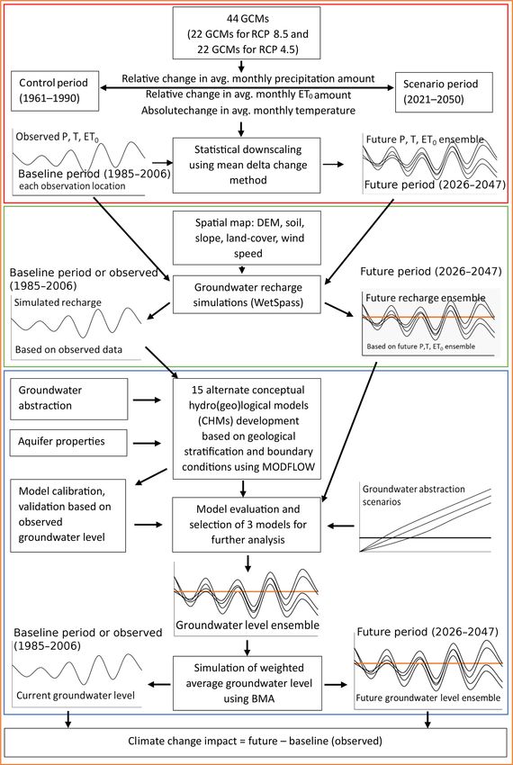
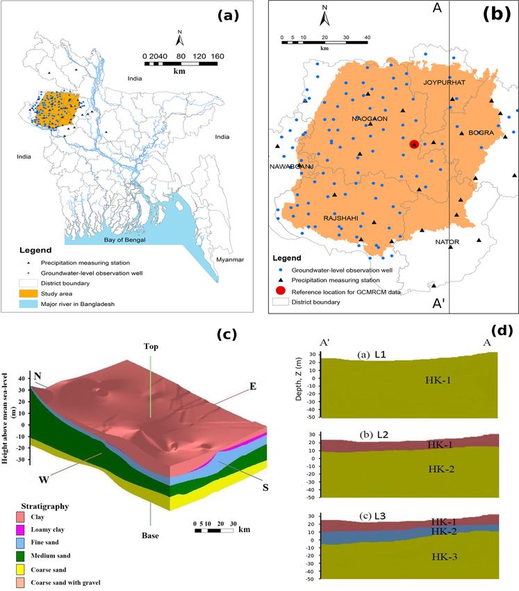
S. M. T. Mustafa et al.: Multi-model approach to quantify groundwater-level prediction uncertainty                           2281

and internal variability (Hawkins and Sutton, 2009; Tebaldi       groundwater levels. The specific objectives to achieve the
and Knutti, 2007). Using an ensemble of climate scenarios         general goal of this study are to (i) quantify the groundwater-
has become common practice in analysis of climate change          level prediction uncertainties arising from the definition of
impact in the field of hydrology. Uncertainty analysis of         alternative CHMs; (ii) analyse the effect of climate change on
groundwater simulations related to climate change has re-         the groundwater levels using ensemble global climate mod-
ceived relatively limited attention (Goderniaux et al., 2009;     els and estimate the uncertainty linked to climate scenar-
Taylor et al., 2013). Holman et al. (2012) recommended that       ios; (iii) analyse the effect of groundwater abstraction sce-
climate scenarios from multiple GCMs or RCMs should be            narios on the future groundwater levels; (iv) quantify the
used to predict the impact of climate change on groundwa-         amount of water that can be abstracted sustainably for ir-
ter. Recently, several researchers have studied the impact of     rigated agriculture in the northwestern part of Bangladesh;
climate change on the groundwater system, incorporating un-       (v) evaluate the combined effect of CHM structure and the
certainty from the input of different GCM or RCM scenarios        climate change and groundwater abstraction scenarios on fu-
and different greenhouse gas emission scenarios (Ali et al.,      ture groundwater-level prediction uncertainty; and (vi) com-
2012; Dams et al., 2012; Jackson et al., 2011; Neukum and         pare the uncertainty arising from the alternative CHMs and
Azzam, 2012; Stoll et al., 2011; Sulis et al., 2012). The un-     climate scenarios and abstraction scenarios.
certainty analysis is, however, usually limited to the climatic
part. Very recently, Goderniaux et al. (2015) included uncer-
tainty related to model calibration in predicting groundwa-       2     Methodology
ter flow along with uncertainty from the GCMs and RCMs
and downscaling methods. However, the uncertainty arising         2.1    Study area
from other sources, such as the model conceptualization and
abstraction scenarios, is not evaluated.                          The study area is located in the northwestern part of
   Groundwater levels are often heavily influenced by the         Bangladesh (Fig. 1a). The study area is a subtropical region
groundwater abstraction rate. For example, in the Indian sub-     with two distinct seasons: the dry winter season (Novem-
continent, groundwater abstraction has increased from 10–         ber to April) and the rainy monsoon season (May to Oc-
20 km3 /year to approximately 260 km3 /year during the last       tober). The average annual precipitation amount varies be-
50 years (Shamsudduha et al., 2011). In the northwestern part     tween 1400 and 1550 mm, but is not uniformly distributed
of Bangladesh, about 97 % of the total groundwater abstrac-       over the year (Fig. S2 in the Supplement). Almost 83 % of
tion is used for irrigated agriculture (Mustafa et al., 2017b;    the total annual amount occurs in the monsoon season. The
Shahid, 2009). Shahid (2011) found an increasing trend in         average temperature varies between 25–35 ◦ C for March to
irrigation application rate in Boro rice, the major irrigated     June and 9–15 ◦ C for November to February. Groundwater
crop in the area. Details on current groundwater abstraction,     depth in the study area is continuously increasing (Fig. S3).
trends in the abstraction and irrigated area can be found in      The study area consists of six northwestern districts (Ra-
Mustafa et al. (2017b). This increasing trend is ascribed to      jshahi, Naogaon, C’Nawabganj, Joypurhat, Bogra and Na-
climate change. In contrast, improvement in agricultural wa-      tor) and covers about 7112 km2 . In comparison to other dis-
ter use efficiency can reduce the water use in irrigated agri-    tricts of Bangladesh, these districts are more affected by
culture. Therefore, multiple abstraction scenarios should be      drought (Shahid and Behrawan, 2008). The study area is sit-
used to predict a reliable uncertainty band.                      uated between latitude 24◦ 190 000 to 25◦ 120 000 N and longitude
   Existing literature on future groundwater-level prediction     88◦ 60 3600 to 89◦ 310 1200 E. The surface elevation in the study
uncertainty quantification has focused on hydrological model      area varies from 11 to 40 m (Fig. S1). There is a mild gradi-
calibration and climate model uncertainty considering one         ent towards the southeastern corner, and this corner is close
single CHM and parameter uncertainty. As far as the au-           to a large wetland.
thors are aware, little research has been done so far to quan-       The aquifer in the study area is comprised of several lay-
tify future groundwater-level prediction uncertainty consid-      ers such as clay, loamy clay, fine sand, medium sand, coarse
ering the uncertainty arising from the CHM structure, climate     sand and gravel with a dominance of medium to coarse sand
change and groundwater abstraction scenarios. This is the         (Fig. 1c). The thickness of each stratigraphic unit more-
first attempt to evaluate the combined effect of CHM struc-       over varies spatially. The top layer consists of clay, clayey
ture and the climate change and groundwater abstraction sce-      loam and fine sand with an average thickness of 18 m. It is
narios on future groundwater-level prediction uncertainty.        underlain by a 20 m thick medium sand layer. Below the
   The general objective of this study is to quantify             medium sand layer, a 35 m thick layer of coarse sand and
groundwater-level prediction uncertainty in climate change        coarse sand with gravel is present. The upper aquifer is un-
impact studies using a multi-model ensemble, i.e. an ensem-       confined or semi-confined with a thickness ranging from 10
ble of representative concentration pathways, global climate      to 40 m (Asad-uz-Zaman and Rushton, 2006; Faisal et al.,
models, multiple alternative CHMs and abstraction scenar-         2005; Jahani and Ahmed, 1997; Michael and Voss, 2009b;
ios to provide probabilistic and informative predictions of       Rahman and Shahid, 2004). The area is dominated by agri-

www.hydrol-earth-syst-sci.net/23/2279/2019/                                    Hydrol. Earth Syst. Sci., 23, 2279–2303, 2019
2282                  S. M. T. Mustafa et al.: Multi-model approach to quantify groundwater-level prediction uncertainty

Figure 1. Description of the study area: (a) location of the study area in the northwestern part of Bangladesh; (b) study area with precipitation
measurement stations (triangles) and groundwater observation wells (circles); (c) stratigraphy of the study area; (d) cross-sectional (A–A’)
view of different models: (a) one-layered model (L1), (b) two-layered model (L2), and (c) three-layered model (L3).

Hydrol. Earth Syst. Sci., 23, 2279–2303, 2019                                             www.hydrol-earth-syst-sci.net/23/2279/2019/
S. M. T. Mustafa et al.: Multi-model approach to quantify groundwater-level prediction uncertainty                           2283

culture and almost 80 % is crop land. Irrigated agriculture        tributed three-dimensional finite-difference numerical flow
plays an important role in the food production and secu-           model developed by the U.S. Geological Survey (USGS).
rity of Bangladesh, home to over 150 million people. In the        MODFLOW solves the three-dimensional partial-differential
northwestern part of Bangladesh irrigated agriculture is the       groundwater flow equation for porous media using a finite-
major user of groundwater and accounts for 97 % of total           difference method.
groundwater abstraction (Shahid, 2009). Overexploitation of
groundwater for irrigation, particularly during the dry sea-       2.4   Multi-step multi-model methodology
son, causes groundwater-level decline in areas where abstrac-
tion is high and surface geology inhibits direct recharge to the   A four-step methodology was used to achieve the objectives
underlying shallow aquifer (Mustafa et al., 2017b).                of the study (Fig. 2). In the first step, the climate model data
                                                                   for precipitation, minimum, mean and maximum tempera-
2.2   Data                                                         ture and ET0 were extracted and downscaled as explained in
                                                                   Sect. 2.6. In the second step, monthly groundwater recharge
Thirty-two years (1979–2011) of weekly groundwater-level           was simulated using a spatially distributed water balance
and daily precipitation data of the Bangladesh Water Devel-        model (WetSpass) (Abdollahi et al., 2017; Batelaan and De
opment Board (BWDB) and Bangladesh Meteorological De-              Smedt, 2001) for the baseline period and for different sce-
partment (BMD) were collected from the Water Resources             narios as explained in Sects. 2.5.2 and 2.7. In the third step,
Planning Organization (WARPO), Bangladesh, for, respec-            15 alternative conceptual hydrogeological models were con-
tively, 140 and 30 sites in the study area. Available river dis-   structed using different geological interpretations and bound-
charge data of the BWDB for the existing small rivers within       ary conditions. All alternative CHMs were calibrated using
the study area were also collected from WARPO. Daily min-          observed groundwater-level data. The performance of each
imum and maximum temperature, wind speed and other cli-            model was evaluated based on different performance eval-
matic data were collected from the BMD for all the available       uation coefficients and information criterion statistics. The
stations in the country. Reference evapotranspiration (ET0 ),      Bayesian model averaging (BMA) method was applied to ob-
considered potential evapotranspiration in this study, was cal-    tain an average prediction from the alternative models. Also,
culated using the FAO Penman–Monteith equation from the            the performance of alternative models was evaluated based
observed climatic data (Allen et al., 1998; Mustafa et al.,        on the maximum likelihood BMA weight of each model. The
2017b).                                                            better-performing models among the alternative models were
   The monthly observed groundwater head data of 50 obser-         used to project groundwater levels under different climatic
vation wells were used for model calibration and validation        and abstraction scenarios. The averaged projection and its
and are plotted in a box-plot (Fig. S2). The groundwater lev-      uncertainty were estimated using BMA of the ensemble of al-
els vary between 3 and 22 m above mean sea level (a.m.s.l.)        ternative CHMs. In the final step, climate change impact was
and display a clear seasonal variation. The groundwater level      assessed. The details of the different materials and methods
is relatively low in April and high in October.                    of each step are described in the following sections.
   The hydraulic properties of the aquifers were selected
based on observed data and previous reports on the geology         2.5   Alternative conceptual groundwater flow models
and lithology of the study area (Michael and Voss, 2009a,
b). Topography and borehole data were collected from               To estimate the uncertainty due to the conceptualization of
the Barind Multipurpose Development Authority (BMDA),              groundwater models, 15 different alternative CHMs were de-
Bangladesh. The log data from 23 boreholes within the study        veloped based on geological stratification and boundary con-
area were collected from the BMDA.                                 ditions. The cross-sectional (A–A’) view of the models is
   The climate model data are available through the website        shown in Fig. 1d. First, three simplified alternative concep-
of the Earth System Grid Federation (https://esgf.llnl.gov,        tual groundwater models were defined based on the geolog-
last access: 8 May 2019).                                          ical stratification. The three models are a one-layered (L1),
                                                                   two-layered (L2) and three-layered (L3) model. In the one-
2.3   MODFLOW model                                                layered model (L1), the entire model domain was considered
                                                                   as one hydro-stratigraphic unit and the hydraulic properties
Processing MODFLOW or PMWIN (Chiang and Kinzel-                    are assumed homogeneous and isotropic. The two-layered
bach, 1998) is a physically based, fully distributed, grid-        model (L2) consists of two layers where the average thick-
based, integrated simulation system for modelling ground-          ness of the top layer was 10 m (clay and loamy clay soil) and
water flow and pollution. PMWIN was designed as a pre-             the rest of the thickness was considered as the bottom layer.
and post-processor for groundwater flow model MODFLOW              The model domain was divided into three different hydro-
(Harbaugh and McDonald, 1996; McDonald and Harbaugh,               stratigraphic units to develop a three-layered model (L3). Be-
1988) to bring various codes together in a simulation sys-         low the top layer, a fine sand layer with an average thickness
tem. The MODFLOW model is a physically based, fully dis-           of 8 m was added in the three-layered model. The bottom

www.hydrol-earth-syst-sci.net/23/2279/2019/                                     Hydrol. Earth Syst. Sci., 23, 2279–2303, 2019
2284                 S. M. T. Mustafa et al.: Multi-model approach to quantify groundwater-level prediction uncertainty

Figure 2. Multi-step multi-model methodology. GCM: general circulation model; RCP: representative concentration pathway; ET0 : potential
evapotranspiration; P : precipitation; T : temperature; DEM: digital elevation model; BMA: Bayesian model averaging.

layer of the three-layered model consists of medium sand,             the other hand, there is a large wetland at the southeast-
coarse sand and coarse sand with gravel.                              ern corner of the study area as well as a large river (known
   Boundary conditions strongly influence the CHM uncer-              as Ganges/Padma) within a few kilometres of the southern
tainty (Wu and Zeng, 2013). They are often very uncertain,            boundary. Since exact boundary conditions were not known,
and, moreover, strongly influence the model results. Previ-           based on the above information, five different potential sets
ous studies in the Bengal Basin (Michael and Voss, 2009a,             of boundary conditions were conceptualized and shown in
b) identified a north-to-south groundwater flow direction. On         Fig. 3. For boundary condition B1, a no-flow boundary con-

Hydrol. Earth Syst. Sci., 23, 2279–2303, 2019                                        www.hydrol-earth-syst-sci.net/23/2279/2019/
S. M. T. Mustafa et al.: Multi-model approach to quantify groundwater-level prediction uncertainty                         2285

dition was assumed on every side of the model. In other          1998; Johnson, 1967) and previous research findings in the
words, there is no interaction between the model domain and      study area (Michael and Voss, 2009a, b). They are listed
the environment (Michael and Voss, 2009a, b). For bound-         in the Supplement. Michael and Voss (2009a) used 9.4 ×
ary condition B2, a constant head boundary is assumed at the     10−5 m−1 as a specific storage value for the Bengal Basin.
northern side where most of the river branches originated,       The initial specific storage was taken as 9.4×10⁻⁵ m−1 when
assuming that groundwater flow direction is parallel to the      it is within the specific storage limits of the aquifer materi-
river flow and perpendicular to the model boundary. No-flow      als according to the literature. Otherwise, the initial specific
boundary conditions were assumed for all other sides. For        storage was taken as the average of the maximum and min-
boundary condition B3, a constant head boundary was con-         imum values of the aquifer materials found in the literature.
sidered on the northern side like for B2 and the southeastern    The rivers in the study area are typically small and mainly
side, i.e. the side where a large wetland is located. Boundary   driven by precipitation runoff. Generally, there is no flow in
condition B4 is based on boundary condition B3. The con-         the rivers during dry months (January to March). The “River
stant head boundary in the southeastern part of the model was    flow package” of MODFLOW was used to define rivers in
extended to the southern part of the model domain in bound-      the model domain and a third-type boundary condition was
ary condition B4 because the great Ganges/Padma River is         assumed for the rivers. Riverbed conductance is indeed de-
very near to the southern boundary. In boundary condition        fined as a lumped parameter in MODFLOW defined as
B5, a constant head boundary was considered at the north-
ern and northwestern boundary and also at the southeastern
                                                                          Kriv × L × W
corner of the model domain based on the information that         CRIV =                ,                                     (1)
groundwater is flowing from north and northwest to south                       Mriv
(Michael and Voss, 2009a, b). A constant head is assigned        where CRIV is riverbed hydraulic conductance (L2 T −1 ),
at the southeastern corner of the model domain represent-        Kriv is riverbed sediment hydraulic conductivity (LT −1 ), L
ing the Chalan Beel wetland as well. No-flow boundaries are      is length of the river within a grid cell (L), W is width of
assumed at the southern and northeastern boundaries since        the river within a grid cell (L) and Mriv is thickness of the
these boundaries are parallel to the groundwater flow direc-     riverbed within a grid cell (L).
tion (Michael and Voss, 2009a, b). The long-term monthly            From the equation, it is clear that riverbed hydraulic
average groundwater levels (normal) were considered as the       conductance depends on grid size, riverbed sediment hy-
constant groundwater heads for the constant head boundary.       draulic conductivity and thickness of the riverbed. Mehl and
As there is seasonal variability in the groundwater level of     Hill (2010) have reported that riverbed conductance depends
this study area, every month was assigned a different con-       heavily on the grid size of the model. Due to a lack of field
stant groundwater head corresponding to the long-term aver-      data for riverbed materials, the riverbed conductance was ob-
age groundwater level for that month.                            tained through manual calibration: riverbed conductance is
   In total, 15 alternative groundwater models were devel-       0.18 m2 s−1 , while riverbed thickness is 0.5 m.
oped using 5 different boundary conditions and 3 different
layer types. A list of the 15 models is included in Table S1.    2.5.2   Simulation of spatially distributed groundwater
                                                                         recharge
2.5.1   Model setup
                                                                 Spatially distributed monthly groundwater recharge was sim-
The BIock Centered Flow Package (BCF) of MODFLOW-96              ulated using the WetSpass-M model (Abdollahi et al., 2017;
within the PMWIN interface was used for groundwater flow         Batelaan and De Smedt, 2001) on the same grid as the
simulation. The study area covers an area of 7112 km2 dis-       groundwater flow (MODFLOW) model. WetSpass-M is a
cretized into smaller cells with 117 rows and 118 columns.       physically based distributed model, in which the groundwa-
The grid cell dimension is 900 m ×900 m. All models are          ter recharge is estimated from a grid-based water balance. To
transient with a monthly time step. A no-flow boundary           allow land cover heterogeneity within each cell, every raster
is considered at the model domain bottom as the vertical         cell is split into four fractions: vegetated, bare-soil, open-
groundwater flow is restricted by the relatively impermeable     water and impervious. The water balances of each fraction
hard rock below the aquifer in the study area. On the model      are used to calculate the total water balance of a raster cell,
top surface, a spatially distributed recharge boundary is con-   whereas recharge is calculated as the residual term of the
sidered.                                                         water balance for each cell. The inputs of the model are spa-
   The initial groundwater heads correspond to a long-term       tially distributed maps of land cover, soil texture, topography,
average groundwater table obtained by running the models         groundwater depth and climatic data. Precipitation (includ-
in steady-state conditions.                                      ing of rainy days), ET0 , temperature and wind speed were
   The range of hydrogeological parameter values was             used as climatic information. Details on model setup and
selected based on typical values for aquifer materials           data preparation for groundwater recharge calculation data
(Domenico and Mifflin, 1965; Domenico and Schwartz,              can be found in Mustafa et al. (2017b). Monthly groundwater

www.hydrol-earth-syst-sci.net/23/2279/2019/                                   Hydrol. Earth Syst. Sci., 23, 2279–2303, 2019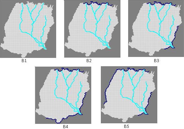
2286                 S. M. T. Mustafa et al.: Multi-model approach to quantify groundwater-level prediction uncertainty

Figure 3. Boundary conditions used to develop alternative conceptual models (dark blue line indicates a constant head boundary). B1: no-
flow boundary; B2: constant head at the northern boundary; B3: constant head at the northern and southeastern boundaries; B4: constant
head at the northern, southern and southeastern boundaries; B5: constant head at the northern, northwestern and southeastern boundaries.

recharge was simulated for 22 years (1985–2006) and con-              2.5.4   Calibration and validation of alternative CHMs
sidered the baseline groundwater recharge.
                                                                      All alternative CHMs were calibrated for the period 1990–
2.5.3   Groundwater abstraction estimation                            1994. Model parameters were estimated using manual cal-
                                                                      ibration and automatic calibration. During auto-calibration,
                                                                      PEST (Doherty, 1994) was used to optimize the model pa-
Groundwater abstraction for irrigation was calculated from            rameter values.
the available data. Unfortunately, detailed groundwater ab-              The initial values, allowable ranges and optimized values
straction information, e.g. amounts of water pumped from              of the parameters of the different models are given in the
individual wells, co-ordinates of the abstraction wells, capac-       Supplement (Tables S2, S3, S4). One-layered-type models
ity of the pumps or duration of pumping, were not available.          were calibrated for three parameters: horizontal hydraulic
Hence, the groundwater abstraction was assessed based on              conductivity, specific storage and specific yield. The two-
the irrigated area by shallow tube wells (STWs), deep tube            layered and three-layered models were calibrated for, respec-
wells (DTWs) and other irrigation equipment. Upazila-wise             tively, 8 and 12 parameters. The process of selecting ini-
(an upazila is the second lowest tier of regional adminis-            tial values and the allowable range of the different param-
tration in Bangladesh) yearly seasonal groundwater abstrac-           eters is described in Sect. 2.5.1. The optimized horizontal
tion for irrigation from the groundwater was calculated using         hydraulic conductivity of the one-layered models varies be-
an empirical equation based on Boro rice irrigation require-          tween 4.45×10⁻³ and 6.00×10⁻³ m s−1 . This high value of
ments and the irrigated area. The irrigation water withdrawal         horizontal hydraulic conductivity corresponds to well-sorted
was considered to be the total abstraction for each upazila. To       coarse sand and gravel (Fetter, 2001). We consider these val-
obtain monthly abstraction for each upazila, the calculated           ues to be realistic since a major portion of the aquifer consists
seasonal abstraction values are initially equally divided over        of coarse sand and coarse sand with gravel. The average hor-
the months of the dry seasons (November to April). Also,              izontal hydraulic conductivity of the Bengal Basin found by
as the location of the pumps is unknown, the total abstrac-           Michael and Voss (2009a) was also high (5 × 10⁻⁴ m s−1 ).
tion from each upazila is initially considered uniformly dis-         They also reported that, based on the drill-log analysis, hor-
tributed over the full upazila. Considering the individual up-        izontal hydraulic conductivity of the Bengal Basin may vary
azila as 1 zone of abstraction, a total of 34 abstraction zones       from 6 × 10⁻⁶ to 3.00 × 10⁻³ m s−1 . The area of the Ben-
were considered. Details on the irrigation data can be found          gal Basin is about 2.8 × 10⁵ km2 , but the study area is only a
in Mustafa et al. (2017b) and Shamsudduha et al. (2015).              small part of the Bengal Basin. Therefore, it is possible that

Hydrol. Earth Syst. Sci., 23, 2279–2303, 2019                                        www.hydrol-earth-syst-sci.net/23/2279/2019/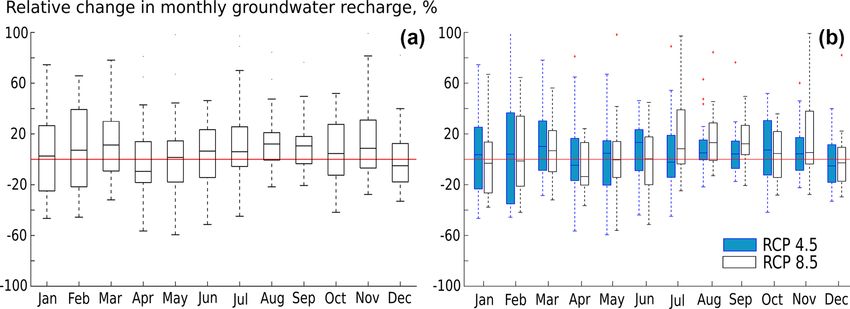
S. M. T. Mustafa et al.: Multi-model approach to quantify groundwater-level prediction uncertainty                          2287

the horizontal hydraulic conductivity is relatively higher in      2.5.5   Model performance evaluation
our study area. Bonsor et al. (2017) have also reported in their
review that aquifer materials in the Bengal Basin are highly       The performance of alternative conceptual groundwater
permeable. Mustafa et al. (2018) have also reported that the       models (CHMs) was evaluated using information criteria,
average horizontal hydraulic conductivity of this study area       statistical indicators and graphical presentation of simulated
is high and around 2.5 × 10⁻³ and 4.5 × 10⁻³ m s−1 .               groundwater levels. Root mean square error (RMSE) and
   Additionally, spatial variability of horizontal hydraulic       Nash–Sutcliffe efficiency (NSE, Eq. 2) of the alternative
conductivity has not been considered in this study. We con-        CHMs were calculated using the formula reported by Mo-
sider an average horizontal conductivity for all individual        riasi et al. (2007). The notation of Mustafa et al. (2017a) has
layers. This might be another reason for high horizontal hy-       been followed.
draulic conductivity.
   The optimized specific storage of the one-layered model                     Pn
                                                                                     (Oi − Si )2
with boundary condition-5 (L1B5) was 4.92 × 10⁻⁵ m−1 .             NSE = 1 − Pi=1
                                                                              n                                               (2)
Michael and Voss (2009a) also reported a similar specific                         i=1 (Oi   − O)2
storage value (9.4 × 10⁻⁵ m−1 ) for the Bengal Basin. How-
                                                                   Here, Oi and Si represent observed and simulated values,
ever, different conceptual models suggest different specific
                                                                   respectively, O is the mean of Oi and n is the number of
storage values within the typical values for aquifer materials
                                                                   observations.
depending on the number of layers and boundary conditions
                                                                      NSE varies from −α to +1 and is dimensionless. NSE
(Tables S2, S3, S4).
                                                                   values closer to 1 mean better simulation efficiency. NSE
   The optimized value of specific yield varies between 0.17
                                                                   values >0.7, 0.35–0.7, 0.0–0.35 and
2288 S. M. T. Mustafa et al.: Multi-model approach to quantify groundwater-level prediction uncertainty
The different information criterion values were obtained reference location is set at 24.81◦ N and 88.95◦ E and is in-
from MODFLOW by running PEST in sensitivity analy- dicated by a red dot in Fig. 1b. Using the FAO Penman–
sis mode. The best model among the alternative CHMs has Monteith equation based on the temperature from climate
a minimum information criterion value (minimum AIC or model data, ET0 is calculated.
AICc or BIC or KIC) (Zhou and Herath, 2017). A poste- Within this case study, CMIP5 (Coupled Model Intercom-
rior model probability (pk ) was calculated using Eq. (8) for parison Project Phase 5) climate model runs for RCP 4.5 and
each information criterion method for each alternative CHM. RCP 8.5 are considered (Taylor et al., 2012; Van Vuuren et
The posterior model probability was used to select the best al., 2011). RCP 8.5 is the highest RCP-based GHS and con-
CHMs. The better model corresponds to a larger posterior siders a radiative forcing of 8.5 W m−2 by 2100. The cor-
model probability (Zhou and Herath, 2017). responding global temperature rise ranges between 2.6 and
4.8 ◦ C. RCP 4.5 is a more intermediate scenario, whereby
the radiative forcing is limited to 4.5 W m−2 by 2100 and cor-
e−0.51k
pk = P K , (8) responding temperature rise between 1.4 and 3.1 ◦ C (IPCC,
−0.51j
j =1 e 2013). The total climate model ensemble includes 44 runs,
1k = AICk − AICmin , (9) where the RCP 4.5 and RCP 8.5 sub-ensembles each include
22 runs. The considered climate model runs are listed in Ta-
where AICk is the AIC value for model k and AICmin is the ble S7.
minimum AIC values of all models. The value of 1k was Goal number six of the United Nations (UN) sustainable
also calculated for AICc, BIC and KIC. development Goals (SDGs) states “Ensuring availability and
sustainable management of water and sanitation for all by
2.5.6 Bayesian model averaging 2030”. Based on this information, the climate change sig-
nals are defined between 1975 and 2035, where the control
BMA was used to deduce more reliable predictions of and scenario periods range between 1961–1990 and 2021–
groundwater levels than the predictions produced by the in- 2050, respectively. The precipitation and evapotranspiration
dividual groundwater models. Draper (1995) and Hoeting et changes are specified on a relative basis, while for the tem-
al. (1999) present an extensive overview of BMA. Recently, perature changes an absolute basis is considered. Using the
BMA has received attention of researchers of diverse fields delta change method, the climate change signals are applied
because of its more reliable and accurate predictions than to the observed time series (Ntegeka et al., 2014). The delta
other model averaging methods. Vrugt (2016) has developed change method is a simple statistical downscaling method
a model averaging MATLAB toolbox called MODELAVG which applies mean monthly average changes (top box of
for post-processing of forecast ensembles. The MODELAVG Fig. 2).
has different model averaging methods including BMA and
was used in this study. Details of the model averaging method 2.7 Future groundwater recharge scenario
are described in the MODELAVG manual (Vrugt, 2016). The
value of βBMA (maximum likelihood Bayesian weight) was The projected spatially distributed monthly groundwater
used as a criterion to select the better-performing models that recharge was simulated for the 44 projected time series us-
have a significant contribution in model averaging. ing the WetSpass-M model (Abdollahi et al., 2017; Bate-
The general equation used to calculate the weighted av- laan and De Smedt, 2001) as explained in Sect. 2.5.2 and in
erage prediction in various model averaging strategies is as Mustafa et al. (2017b). Details about the considered climate
follows: model runs for this study are explained in Sect. 2.6, and they
are listed in Table S7. The baseline groundwater recharge
K
X was calculated for a period of 22 years (1985–2006). Future
yj =
e βk Dj k , (10) groundwater recharge was simulated for the same number
k=1 of years (2026–2047). Simulated groundwater recharges of
where Dj k is the bias-corrected point forecasts of each the baseline period were compared to the simulated future
model, k = {1, . . . , K} is model number and j = {1, . . . , n} groundwater recharge to estimate the combined influence of
is forecast number, e yj = {e yn } is the weighted average
y1 , . . . , e the greenhouse gas scenarios or representative concentration
forecast for the j th forecast number, and β = {β1 , . . . , βk } pathways, climate models and internal variability.
denotes the weight vector.
2.8 Development of future groundwater abstraction
2.6 Climate change scenarios scenario
The climate model data for precipitation and minimum, mean It is challenging to estimate future groundwater abstraction
and maximum temperature are extracted for the grid cells scenarios because they largely depend on human activities as
covering the reference location within the catchment. This well as on climate. In this study, we have developed differ-
Hydrol. Earth Syst. Sci., 23, 2279–2303, 2019 www.hydrol-earth-syst-sci.net/23/2279/2019/S. M. T. Mustafa et al.: Multi-model approach to quantify groundwater-level prediction uncertainty 2289
ent future abstraction scenarios. The groundwater abstraction narios are developed (Table 1). The first scenario is devel-
data of the study area show a linearly increasing trend during oped based on the current increasing trend. The second sce-
1985 to 2006 (Fig. S4). The increasing rate is different in dif- nario assumes an improved irrigation water use. As such the
ferent groundwater abstraction zones. The average ground- conveyance efficiency will compensate the increasing future
water abstraction rate in 2006 was about 5 times higher than demand and the groundwater abstraction rate will remain
that in 1985. A similar increasing trend in groundwater ab- constant. In other words, this scenario considers the ground-
straction in the study area was also found by Mustafa et water abstraction rate for 2010. The third, fourth and fifth
al. (2017b). Shahid (2011) predicts an increasing trend in scenarios assume, respectively, 30 %, 50 % and 60 % lower
future irrigation application for Boro rice production due to groundwater abstraction, where the groundwater abstraction
climate change. He also predicts that the length of the Boro rate in 2010 was considered as a basis.
rice growing period may decrease in future, which may lead
to increased cropping intensity in the area. Increased crop- 2.9 Uncertainty estimation
ping intensity may increase the overall yearly groundwater
abstraction rate. Moreover, it is estimated that the popula- The spread of the 95 % prediction interval was taken as the
tion of Bangladesh will increase from 145 million in 2008 uncertainty band of the ensemble. The uncertainty band was
to 182 million by 2030 (Qureshi et al., 2014). Thus, wa- estimated using Eq. (11).
ter use for food production will increase tremendously. As
groundwater is the major source of water in the study area,
n n n
the groundwater withdrawal rate will be much higher. Uband = D97.5 − D2.5 , (11)
However, there was no effective groundwater abstraction N
1 X
n
policy before 2017. Recently, the Integrated Minor Irrigation Uavg = Uband , (12)
Policy 2017 and the Groundwater Management Law 2018 N n=1
for agriculture were proposed to ensure sustainable irriga-
n
where Uband is the uncertainty band of a time step, Uavg is
tion management. Both the Integrated Minor Irrigation Pol-
icy 2017 and the Groundwater Management Law 2018 have the average uncertainty band, N is the total number of pre-
n
dictions, and D97.5 n represent the 97.5th and 2.5th
and D2.5
recommended minimizing the groundwater abstraction in the
study area to maintain sustainable groundwater abstraction. percentiles of the ensemble at a time step, respectively.
They also encourage use of surface water instead of ground- In the case of alternative CHM uncertainty quantification,
water for the irrigation. Unfortunately, no quantitative or spe- the same abstraction and recharge scenarios of the baseline
cific action, for example how much abstraction should be re- period were used to simulate groundwater levels of the 22-
duced, has been mentioned either in the proposed Integrated year period. To quantify the recharge scenario uncertainty,
Minor Irrigation Policy 2017 or in the Groundwater Manage- the groundwater level was simulated for 44 recharge scenar-
ment Law 2018. The policy planning and management strate- ios by the best-performing groundwater flow model where
gies should be updated based on the quantitative or specific the groundwater abstraction scenario was kept the same. The
information. groundwater level was simulated for five abstraction scenar-
Groundwater abstraction can be reduced by improving ios by the best-performing groundwater flow model where
agricultural water use efficiency. The agricultural water use the same recharge scenario was used to estimate abstraction
efficiency is extremely low in Bangladesh. On average, crops scenario uncertainty. The groundwater levels in 50 observa-
use only 25 %–30 % of applied irrigation water, and the rest tion wells for a period of 22 years were used to estimate the
is lost due to inefficient irrigation systems (Karim, 1997; spread of the 95 % prediction interval.
Mondal, 2005, 2010). Using efficient irrigation distribution The contribution of the different sources of uncertainty in
and application techniques can increase agricultural water future groundwater-level prediction was calculated consider-
use efficiency. The BMDA has introduced a buried PVC pipe ing all the probable combinations of the CHM, recharge and
water conveyance system in the study area to increase con- abstraction scenarios. The average prediction interval at each
veyance efficiency to more than 90 %, whereas the national time step was calculated using the following equations:
average value is 40 % (Rahman et al., 2011). Alternate wet-
ting and drying (AWD) rice irrigation techniques can save
AS X RS
30 % to 70 % of water compared to conventional irrigation n 1 X
methods (Rahman and Bulbul, 2015). Deficit irrigation in UCM = Un , (13)
avg AS × RS AS=1 RS=1 CMAS, RS
wheat cultivation in the study area can save 121–197 mm of
K X AS
water per season (Mustafa et al., 2017a). Food habit changes 1 X
URnavg = Un , (14)
and/or crop diversification may also have an impact on crop K × AS K=1 AS=1 RK, AS
water use efficiency. K X RS
Considering the uncertainties in the total groundwater ab- 1 X
UAn avg = Un , (15)
straction amount, five different groundwater abstraction sce- K × RS K=1 RS=1 AK, RS
www.hydrol-earth-syst-sci.net/23/2279/2019/ Hydrol. Earth Syst. Sci., 23, 2279–2303, 20192290 S. M. T. Mustafa et al.: Multi-model approach to quantify groundwater-level prediction uncertainty
Table 1. Description of future groundwater abstraction scenarios.
Groundwater abstraction Description
scenario
PLinear Linear increase in groundwater abstraction rate based on current increasing trend
PConstant Groundwater abstraction rate of 2010 assumed to be constant in future
PReduced_30 30 % less groundwater abstraction than in 2010
PReduced_50 50 % less groundwater abstraction than in 2010
PReduced_60 60 % less groundwater abstraction than in 2010
where UCM n , URnavg and UAn avg represent the average predic- jas et al. (2010). In contrast, some of the models did not pre-
avg
tion interval at each time step due to CHMs, recharge sce- dict statistically different results.
nario and abstraction scenario, respectively. The K, AS and
RS represent the number of CHMs, abstraction scenarios and 3.1.1 Goodness of fit of alternative CHMs
recharge scenarios, respectively. The UCM n is the predic-
AS, RS
tion interval due to different CHMs for a particular recharge Based on different statistical coefficients, the performance
and abstraction scenario. The URnK, AS and UAn K, RS represent was different for alternative models, and the models per-
the prediction interval due to different recharge scenario and formed differently in the calibration and validation periods
abstraction scenario, respectively, for a particular CHM and (Table S5).
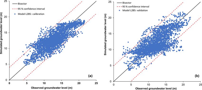
abstraction/recharge scenario. Based on RMSE and the NSE value, the L2B3 model
was the best model in the calibration period, whereas in the
2.10 Data analysis validation period it was L2B5. In general, the two-layered
models had a relatively lower RMSE than the one-layered
Details about the procedure followed for data analysis are and three-layered models. Overall, based on both RMSE and
given in Sects. 2.4 to 2.9. For data analysis and plot- NSE, the two-layered models outperformed the one-layered
ting, different Matlab, R and Python packages were used, and three-layered models in the calibration and validation pe-
such as Pandas (McKinney, 2010), Scipy, ggplot2, Numpy riods.
(Walt et al., 2011) and Matplotlib (Hunter, 2007). The The simplified one-layered models have a comparatively
null hypotheses for equal distributions of simulated ground- higher bias in prediction. Comparatively, a large number of
water levels of alternative CHMs were tested using two- processed parameters made the three-layered models over-
sample Kolmogorov–Smirnov tests (Chakravarti and Laha, parameterized. The three-layered models performed better
1967). The nonparametric modified Mann–Kendall trend test than the one-layered models during calibration, but they per-
(Hamed and Rao, 1998) was conducted to detect trends in formed similarly in most of the cases in the validation period.
annual groundwater level, and the slope was estimated using The performance of the two-layered models also differed be-
Sen’s method (Sen, 1968). tween the calibration and validation periods. It is difficult
to calibrate over-parameterized models efficiently (Willems,
2012), so the two-layered models with eight calibrated pa-
rameters can be a balance between oversimplified and over-
3 Results and discussion parameterized models.
Figure 5 shows the scatter plot for model L2B5. One of
3.1 Groundwater-level simulation the possible causes of the observed differences is the spatial
and temporal variation in groundwater abstraction. The zone-
The simulated groundwater levels of each alternative ground- wise spatially distributed groundwater abstraction rate was
water flow model were compared to the observed groundwa- one of the most important input data in this study. In reality,
ter levels as well as to the simulated groundwater levels of groundwater abstraction varies spatially within those zones.
the other models. The null hypotheses for the equal distribu- Agricultural and industrial areas abstract more groundwa-
tion test between simulation results of alternative models in ter than wetlands or forest areas. Moreover, groundwater
the calibration and validation periods were tested (Fig. 4). A abstraction rate also varies in time following cropping sea-
significant difference (significance level of 0.05 or pS. M. T. Mustafa et al.: Multi-model approach to quantify groundwater-level prediction uncertainty 2291 Figure 4. Significance of difference in simulation results for combinations of alternative conceptual models (p
2292                  S. M. T. Mustafa et al.: Multi-model approach to quantify groundwater-level prediction uncertainty

Figure 5. Scatter plot for the simulated versus observed groundwater level for Model L2B5: (a) calibration period and (b) validation period.

Figure 6. Posterior probability (pk ) and BMA maximum likelihood weight (βBMA ) of alternative models calculated using 10 years of data.
The value above the bar represents the maximum likelihood Bayesian weight.

the prediction of those selected models and the new βBMA                March displays a significant increase. The effect of the GHS
of L1B5, L2B4 and L2B5 was 0.35, 0.39 and 0.26, respec-                 on the monthly precipitation amount changes is shown by
tively. During this recalculation, the 95 % prediction interval         Fig. 7b. One would expect increasing/decreasing change sig-
covers about 82 % of observation data, meaning exclusion of             nals under increasing GHSs. This unidirectional behaviour
12 models resulted in a loss of only 3 % of observed data.              is, however, limited to the months July, August, September
                                                                        and November. Most likely, 2035 is situated before the time
3.2    Climate change impact on precipitation,                          of emergence, whereby the effect of the increasing GHS re-
       temperature and evapotranspiration                               mains mainly masked by noise inherent to the internal cli-
                                                                        mate variability (Hawkins and Sutton, 2012). This, more-
Figure 7 shows the changes in monthly climatic parameters               over, indicates that the months July, August, September and
between the control and scenario periods ranging between                November are most likely more sensitive to the GHSs com-
1961–1990 and 2021–2050, respectively. Figure 7a shows                  pared to the other months.
the changes in the monthly precipitation amount. Small pos-                Figure 7c presents the climate scenarios for minimum,
itive changes in monthly precipitation amounts are observed             mean and maximum daily temperature. It shows the abso-
for the wet season. For the dry season (November to April),             lute changes in monthly minimum, mean and maximum daily
in contrast, the changes are less consistent: decreasing pre-           temperature between the control and scenario periods. Gen-
cipitation amounts are found for April and December, while

Hydrol. Earth Syst. Sci., 23, 2279–2303, 2019                                          www.hydrol-earth-syst-sci.net/23/2279/2019/
S. M. T. Mustafa et al.: Multi-model approach to quantify groundwater-level prediction uncertainty 2293
Figure 7. Climate impact signal for all selected climate models (1975–2035): (a) relative changes in monthly precipitation amount (all GHSs
combined), (b) relative changes in monthly precipitation amount as a function of the GHSs, (c) absolute changes in monthly minimum, mean
and maximum daily temperature (all GHSs combined), and (d) relative changes in potential evapotranspiration as a function of the GHSs.
erally, higher increases in minimum and mean daily tem- 3.3 Climate change impact on groundwater recharge
peratures are projected during the wet season. An inter-
comparison between the different variables shows, further-
more, higher changes for the minimum daily temperature The changes in the monthly groundwater recharge due to
than for the mean and maximum daily temperature. climate change are highly uncertain (Fig. 8a). Like precip-
The changes in monthly potential evapotranspiration are itation, small increasing changes in monthly groundwater
shown in Fig. 7d. Except for May, increases are observed for recharge are observed for the wet season. For the dry sea-
all months. For some months, the changes seem not sensitive son (November to April), in contrast, the changes are less
to the GHS. Changes for the months March, April, June, Oc- consistent. The majority of the global climate model runs
tober and December seem particularly sensitive to the GHS. project generally an increasing groundwater recharge. How-
Similarly to the precipitation results, a possible explanation ever, for April and December, significant decreases are noted.
can be found in the “time of emergence” concept. The effect of the GHSs on the monthly groundwater recharge
The climate change signals for a representative month in changes is shown by Fig. 8b. The months July, August,
the dry and wet seasons are included in Table S8. September and November seem to be more sensitive to the
GHSs compared to the other months. For both RCP 8.5 and
www.hydrol-earth-syst-sci.net/23/2279/2019/ Hydrol. Earth Syst. Sci., 23, 2279–2303, 20192294 S. M. T. Mustafa et al.: Multi-model approach to quantify groundwater-level prediction uncertainty
Figure 8. Change in groundwater recharge due to climate change: (a) relative changes in monthly groundwater recharge (all GHSs combined);
(b) relative changes in monthly groundwater recharge as a function of the GHSs.
RCP 4.5, April and December show decreasing changes in tially and ranges between 0.05 and 0.49 m/year. Mustafa et
monthly groundwater recharge. al. (2017b) studied observed groundwater-level data of the
Projected spatial variation of the mean groundwater same study area and reported that the average groundwater
recharge change between the future and baseline periods due level dropped by 4.5–4.9 m over the last 29 years at a rate of
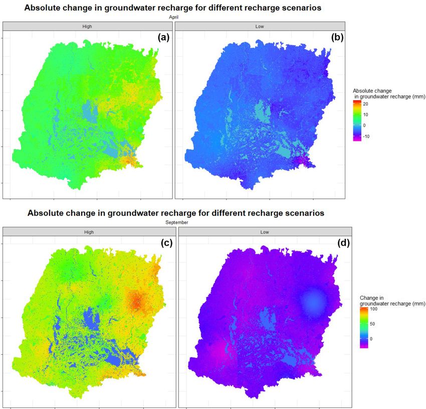
to climate change is presented in Fig. 9. Spatial variation 0.15–0.17 m/year. The annual groundwater-level fluctuation
is observed only for two extreme recharge scenarios: high of 3 to 5 m in the baseline scenario is also supported by the
recharge scenario indicates maximum recharge at each time findings of Shamsudduha et al. (2009). Overall, the simulated
step among all the ensembles and low recharge scenario in- groundwater levels correspond well to the findings of other
dicates minimum recharge. For both April and September, researchers for the baseline period. Therefore, the simulated
the high recharge scenario shows a zero to positive change groundwater level of the baseline period was used for com-
in groundwater recharge, while the low recharge scenario parison with the simulated groundwater levels of the future
shows a zero to negative change in groundwater recharge. scenarios.
No clear spatial trends are observed in the change in ground-
water recharge. In the high recharge scenario, mean monthly 3.4.2 Impact of climate change on groundwater level
groundwater recharge would increase by 25 mm (April) and
100 mm (September). In the low recharge scenario, mean The impact of climate change on groundwater level is highly
monthly groundwater recharge would decrease by 16 mm uncertain in the study area (Fig. 10a). The uncertainty ranges
(April) and 35 mm (September). Crosbie et al. (2010), also, of the change in mean monthly groundwater level due to
reported that changes in groundwater recharge due to climate different GCMs and GHSs obtained from the three selected
change are uncertain. conceptual groundwater flow models are presented with the
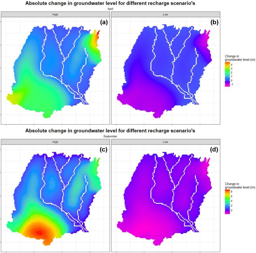
box-plot for each month. Climate change could increase the
3.4 Future groundwater-level analysis
mean monthly groundwater level by up to 2.5 m and could
The baseline and future groundwater levels were simulated decrease it by 0.5 m. However, the SDGs suggest a 0–0.5 m
using three selected groundwater flow models (L1B5, L2B4, increase in groundwater level due to climate change. The im-
L2B5). Then, the model average was calculated by Eq. (1) pact of climate change seems higher from May to Septem-
using simulated groundwater levels and the maximum like- ber than from October to April. This seasonal variation of
lihood Bayesian weight of the respective groundwater flow climate change impact can be explained by the precipita-
models. The change in groundwater level for different sce- tion pattern of the study area (Fig. S2a). Large precipitation
narios is discussed below. amounts occur from May to October in Bangladesh, so that
climate change has a higher impact in this period. Uncer-
3.4.1 Baseline groundwater-level simulation tainty of groundwater level due to climate change is highest
from June to December. The precipitation pattern can also
Groundwater levels in the baseline scenario show a decreas- explain the monthly variation of climate change impact un-
ing trend. The mean decreasing rate of groundwater level certainty. Groundwater levels increase more during the rainy
is 0.18 m/year (Sen’s slope). The summary of the trend season in a high recharge scenario (high precipitation), but
analysis for 50 observation wells is shown in the Supple- in a low recharge scenario, groundwater levels decrease due
ment (Table S9). The calculated decreasing rate varies spa- to the lack of recharge in the rainy seasons. Therefore, the
Hydrol. Earth Syst. Sci., 23, 2279–2303, 2019 www.hydrol-earth-syst-sci.net/23/2279/2019/You can also read