Towards the closure of momentum budget analyses in the WRF (v3.8.1) model
←
→
Page content transcription
If your browser does not render page correctly, please read the page content below
Geosci. Model Dev., 13, 1737–1761, 2020
https://doi.org/10.5194/gmd-13-1737-2020
© Author(s) 2020. This work is distributed under
the Creative Commons Attribution 4.0 License.

Towards the closure of momentum budget analyses
in the WRF (v3.8.1) model
Ting-Chen Chen, Man-Kong Yau, and Daniel J. Kirshbaum
Department of Atmospheric and Oceanic Sciences, McGill University, Montreal, H3A0B9, Canada

Correspondence: Ting-Chen Chen (ting-chen.chen@mail.mcgill.ca)

Received: 22 August 2019 – Discussion started: 23 October 2019
Revised: 25 February 2020 – Accepted: 28 February 2020 – Published: 2 April 2020

Abstract. Budget analysis of a tendency equation is widely       1   Introduction
utilized in numerical studies to quantify different physical
processes in a simulated system. While such analysis is of-      The atmosphere is a complex system with different scales
ten post-processed when the output is made available, it is      of motion. Its dynamics are governed by a set of fluid equa-
well acknowledged that the closure of a budget is difficult      tions based on the fundamental laws of physics. Although the
to achieve without temporal and/or spatial averaging. Nev-       equation set cannot be solved analytically, numerical mod-
ertheless, the development of errors in such calculations has    els can be used to simulate the observed weather and cli-
not been systematically investigated. In this study, an inline   mate systems to improve our understanding of the atmo-
budget retrieval method is first developed in the WRF v3.8.1     sphere. Due to the complexity and nonlinearity of the nu-
model and tested on a 2D idealized slantwise convection case     merical models, budget analysis is often employed to inter-
with a focus on the momentum equations. This method ex-          pret the results by quantifying the contribution of each term
tracts all the budget terms following the model solver, which    (i.e., physical process) in a tendency equation that governs
gives a high accuracy, with a residual term always less than     the evolution of a certain quantity in the simulated system.
0.1 % of the tendency term. Then, taking the inline values       The accuracy of a given budget analysis can be estimated
as truth, several offline budget analyses with different com-    from the residual term, defined as the difference between the
monly used simplifications are performed to investigate how      tendency term on the left-hand side (lhs) of the equation and
they may affect the accuracy of the estimation of individual     the summation of all the forcing terms on its right-hand side
terms and the resultant residual. These assumptions include      (rhs). Budget analysis has been performed on diverse prop-
using a lower-order advection operator than the one used in      erties (e.g., momentum, temperature, water vapor, vorticity)
the model, neglecting grid staggering, or following a mathe-     of many systems on various scales, including the Madden–
matically equivalent but transformed format of the governing     Julian oscillation (MJO; e.g., Kiranmayi and Maloney, 2011;
equations. Errors in these post-processed analyses are found     Andersen and Kuang, 2012), tropical cyclones (e.g., Zhang
mostly over the area where the dynamics are the most ac-         et al., 2000; Rios-Berrios et al., 2016; Huang et al., 2018),
tive, thus impairing the subsequent physical interpretation.     squall lines (e.g., Sanders and Emanuel, 1977; Gallus and
A maximum 99th percentile residual can reach > 50 % of           Johnson, 1992; Trier et al., 1998), supercell thunderstorms
the concurrent tendency term, indicating the danger of ne-       (e.g., Lilly and Jewett, 1990), and so on.
glecting the residual term as done in many budget studies.          Despite the popularity of the budget analysis, it is gener-
This work provides general guidance not only for budget di-      ally acknowledged that, in model post-processing analysis,
agnoses with the WRF model but also for minimizing the           obtaining a closed budget with a negligible residual is diffi-
errors in post-processed budget calculations.                    cult (e.g., Kanamitsu and Saha, 1996) and has been accom-
                                                                 plished mostly in time- or domain-averaged budget calcula-
                                                                 tions (e.g., Lilly and Jewett, 1990; Balasubramanian and Yau,
                                                                 1994; Arnault et al., 2016; Kirshbaum et al., 2018; Duran and
                                                                 Molinari, 2019). Even in the case of averaged budgets, the

Published by Copernicus Publications on behalf of the European Geosciences Union.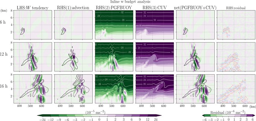
1738                                               T.-C. Chen et al.: Momentum budget analyses in the WRF (v3.8.1) model

residual term that contains non-explicitly diagnosed physics       non-dominant terms may be as important as the large forcing
can be larger than the tendency term (e.g., Liu et al., 2016),     terms in determining the sign and the value of the tendency.
and many studies simply do not display the residual, making        Thus, an incorrect estimation of even a small term may re-
the proper interpretation of the budget analysis difficult.        sult in a residual with magnitude comparable to the tendency
   The “residual analysis method” is sometimes utilized to         term, hindering the subsequent physical interpretation.
obtain an indirect estimation of the physical processes that          A few models, such as the Cloud Model 1 (CM1; Bryan
are hard to diagnose or are unresolved in a set of analysis        and Fritsch, 2002) and the High Resolution Limited Area
or observational data. In such cases, a non-negligible resid-      Model (HIRLAM; Undén et al., 2002), include inline bud-
ual is sometimes used to gain insight into such processes.         get diagnoses that users can choose to include in the
However, as just discussed, the residual term also contains        model output. However, many other commonly used models
the inaccuracies associated with the calculations within the       (e.g., Fifth-Generation NCAR/Penn State Mesoscale Model
budget analysis (e.g., Kornegay and Vincent, 1976; Abarca          (MM5; Grell et al., 1994), Weather Research and Forecasting
and Montgomery, 2013). It is thus unclear whether the un-          Model (WRF; Skamarock et al., 2008), the Advanced Re-
resolved physics in such data sets do indeed comprise the          gional Prediction System (ARPS; Xue et al., 2000, 2001),
main component of the residual without considering the con-        and the Regional Atmospheric Modeling System (RAMS;
tributions of other sources of errors in the budget calculation    Pielke et al., 1992)) do not have this capability. In this study,
(Kuo and Anthes, 1984). Whereas it is almost impossible to         we develop an inline momentum budget retrieval tool in the
separate the subgrid-scale, unresolved processes from other        Advanced Research WRF model, one of the most widely
errors in reanalysis or observational data (e.g., Hodur and        used numerical weather prediction models. During the pe-
Fein, 1977; Lee, 1984), the focus of this study is on numer-       riod 2011–2015, there were on average 510 peer-reviewed
ical model data where the local tendency and all the asso-         journal publications involving WRF per year (Powers et al.,
ciated resolved and parameterized physics can be obtained          2017). Given the widespread use of WRF for both real-case
from the model. Thus, the residual term in this study specifi-     and idealized modeling, such a budget tool may prove use-
cally refers to errors in the budget calculation.                  ful in numerous applications. In our budget diagnosis, each
   To reduce the residual, an inline budget analysis that ex-      contributing term is extracted during the model integration
tracts all the terms of a prognostic equation directly from        and stored as a standard output. In so doing, we essentially
the model during its integration is generally the most accu-       solve the prognostic variables as done in the model so that
rate. However, the procedure has been reported only in a few       the two sides of the tendency equation are always in balance
studies (e.g., Zhang et al., 2000; Lehner, 2012; Moisseeva,        regardless of the output time interval. By taking the results
2014; Moisseeva and Steyn, 2014; Potter et al., 2018; see          from the inline budget analysis as truth, we then perform
Appendix A for a summary and comparison among these                several different post-processing budget analyses with com-
works). Most other studies still conduct the offline or post-      monly made simplifications or a different format of equation.
processing budget analysis when the output is made avail-          Comparisons between the post-processed budgets and the in-
able after the model integration. Some specific suggestions        line/true values are made to investigate the potentially large
have been given in the past regarding how to reduce the er-        errors in each forcing term and the resultant residuals.
ror of post-processed budget analysis. For example, Lilly and
Jewett (1990) emphasized the importance of evaluating terms
using the same differencing scheme, grid stretching, and grid      2     Model and numerical setup
staggering as that used in the simulation model. However, it
                                                                   2.1    Model and momentum equations
is uncertain whether these rules have been widely followed,
and how much of a reduction in residual can be obtained with       The WRF configuration used in this study is a two-
this approach.                                                     dimensional [(y, z); no variation in the x direction], fully
   In some post-processed budget analyses, transformed             compressible, non-hydrostatic, and idealized version of the
equations with different assumptions from those in the model       Advanced Research WRF model, version 3.8.1 (Skamarock
are used and naturally lead to errors in the budget results. On    et al., 2008). Here we briefly revisit the parts that are rele-
the other hand, even when the same form of the equations           vant to the momentum budget analysis. The governing equa-
is followed, errors can still arise from multiple sources dur-     tions in the WRF model are cast on a terrain-following dry-
ing the post-processing. Some errors are inherent in the time      hydrostatic pressure coordinate. This vertical coordinate, η,
discretization scheme of the model, some are traced to the         is defined as
numerical methods in solving the temporal or spatial deriva-
tives with finite differencing (e.g., Kuo and Anthes, 1984),

                                                                   η = pdh − pdh_top /µd ,
and others might emerge during the interpolation or extrapo-
lation from model grids to analysis grids (e.g., Lilly and Jew-    where pdh is the hydrostatic pressure of the dry air and µd
ett, 1990). While the tendency term is often the result of a few   represents the mass of the dry air per unit area in the column;
cancelations among competing forcing terms, the seemingly          µd = pdh_sfc − pdh_top , where pdh_sfc and pdh_top indicate the

Geosci. Model Dev., 13, 1737–1761, 2020                                              www.geosci-model-dev.net/13/1737/2020/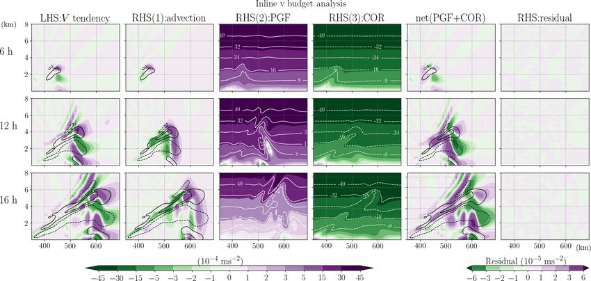
T.-C. Chen et al.: Momentum budget analyses in the WRF (v3.8.1) model                                                          1739
                                                                                                         −1
values of pdh at the surface and the top of the dry atmosphere,    αd 1 + qv + qc + qr + qi + qs + qg , where qv , qc , qr , qi ,
respectively.                                                      qs and qg are the mixing ratios for water vapor, cloud, rain,
   To ensure conservation properties, the model equations are      ice, snow, and graupel, respectively. The rhs forcing terms for
formulated in flux form, with the prognostic variables cou-        the V tendency include the flux-form advection (ADV), hor-
pled with µd . The flux-form momentum components are de-           izontal pressure gradient force (PGF), Coriolis force (COR),
fined as                                                           vertical (earth-surface) curvature (CUV), and the remaining
                                                                   physics (PV ). For the W tendency, the rhs forcings contain
                                                   dη
U = µd u,     V = µd v,     W = µd w,      = µd      ,            the flux-form advection (ADV), net force between the ver-
                                                   dt              tical pressure gradient and buoyancy (PGFBUOY), curva-
where u, v, and w are the two horizontal and vertical veloc-       ture effect (CUV), and the remaining physics (PW ). The re-
ities, respectively. Note that the dry-mass-coupled velocities     maining physics may include diffusion, damping processes,
(U , V , W ) on coordinates (x, y, z) have units of pascal meter   and other parameterized physics, depending on the model
per second, and the dry-mass-coupled vertical velocity on η        setup. Note that for closing the budget analysis, all the known
coordinate, , has a unit of pascal per second. For the ideal-     physics processes that come into play should be explicitly
ized 2D case on an f plane as in this study, the momentum          written in the equation and be diagnosed or directly retrieved
equations in the WRF model are written as                          from the model. The residual (res) is added on the last rhs
                                                                   term in Eqs. (1) and (2) to represent the imbalance between
   ∂V                                ∂p    α ∂p ∂φ                 the two sides of the equation during budget analysis, but it is
           = −∇ · (V v)       −µd α     −
   ∂t
  |{z}
              | {z }                 ∂y αd ∂η ∂y                   not part of the original equations solved in the model.
               advection                                              To develop an inline budget retrieval tool, it is important
                              |         {z         }
V tendency
                         horizontal pressure gradient force        to understand how these prognostic variables are advanced
                 ADV
                                        PGF                        in the WRF model. Governing equations are first recast to

               vW
                                                                  perturbation forms with respect to a dry hydrostatically bal-
  −f U −              +        PV        + res,                    anced reference state that is a function of height only (de-
                r
           | {ze }
  | {z }                      |{z}
 Coriolis                   remaining                              fined at initialization) to reduce truncation errors and ma-
            curvature                                              chine rounding errors. Specifically, variables of p, φ, αd , and
   COR                   (parameterized)
              CUV            physics                               µd are separated into reference and perturbation components,
                                                                   e.g., p(x, y, η, t) = p(z) + p 0 (x, y, η, t). The introduction of
                                                             (1)   these perturbation variables only changes the expressions for
                                                                   the rhs terms PGF and PGFBUOY in Eqs. (1) and (2), which
                                                                   will not be shown here for simplicity. Readers can refer to
  ∂W

                                      α ∂p
                                                                  Skamarock et al. (2008, chap. 2.5) for more details.
           = −∇ · (V w) +         g          − µd                     Based on Skamarock et al. (2008), Fig. 1 summarizes the
   ∂t        | {z }                   αd ∂η
  |{z}
              advection
                                  |       {z      }                WRF integration strategy. The integration is wrapped by a
W tendency
                            net vertical pressure gradient         third-order Runge–Kutta (RK3) scheme, in which the prog-
                 ADV
                                 and buoyancy force                nostic variables (generalized as 8 here) are advanced from t
                                     PGFBUOY                       to t + 1t given their corresponding partial differential equa-
                                                                 tions, ∂8
                                                                          ∂t = F (8), following a three-step strategy:
    uU + vV
+                +       PW          + res,
        r                                                                    1t
       {ze
                         |{z}
|              }
                       remaining                                   8∗ = 8t +     F (8t ),
    curvature                                                                 3
                    (parameterized)                                           1t
      CUV               physics                                    8∗∗ = 8t +     F (8∗ ),
                                                                               2
                                                             (2)   8t+1t = 8t + 1tF 8∗∗ ,

                                                                                                                                 (4)
where                                                              where 1t is the model integration time step and F , the large-
                 ∂ (U a) ∂ (V a) ∂ (a)                            step forcing, represents the summation of all the rhs terms of
−∇ · (V a) = −          −       −                            (3)   Eqs. (1) and (2) excluding the residual. Although the param-
                   ∂x       ∂y     ∂η
                                                                   eterized forcings stay fixed from step one to three as most of
is the flux-form advection, p is the full pressure with in-        the parameterization schemes are called only once at the first
clusion of vapor, φ is the geopotential, f is the Cori-            RK3 step, the rest of the non-parameterized forcings and thus
olis parameter, re is the mean earth radius, and α and             the total F are changed with the updated 8∗ and 8∗∗ at the
αd are the full and dry-air specific volume, respec-               second and third RK3 step. Within each RK3 step, a subset
tively. In our selected microphysics scheme (Thompson et           of integration with a relatively smaller time step is embedded
al., 2008), six hydrometeors are included, and thus α =            to accommodate high-frequency modes for numerical stabil-

www.geosci-model-dev.net/13/1737/2020/                                                Geosci. Model Dev., 13, 1737–1761, 2020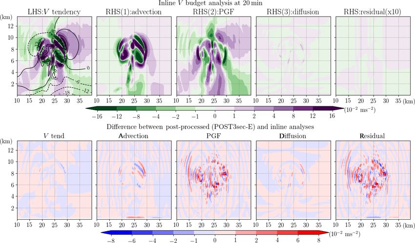
1740 T.-C. Chen et al.: Momentum budget analyses in the WRF (v3.8.1) model
ity (Wicker and Skamarock, 2002; Klemp et al., 2007; Ska- budget retrieval. Note that the overbar in Eq. (6) indicates a
marock et al., 2008). A maximum number of small steps in forward-in-time averaging operator for the small-step modes
one model integration step can be specified by the user. To to damp instabilities associated with vertically propagating
improve accuracy in the temporal solver, the variables be- sound waves (see Eq. 3.19 in Skamarock et al., 2008). Equa-
ing advanced in this small-step integration are the temporal tions (5) and (6) are the ones used to integrate the prognostic
perturbation fields, defined by the deviation from their more momentum fields in the WRF model. For each RK3 step, af-
recent RK3 predictors: 800 = 8 − 8t∗ , where 8t∗ = 8t , 8∗ ter the total large-step forcing F is determined, V 00 and W 00
and 8∗∗ for the first, second, and third RK3 step, respec- are defined and advanced within the small-step scheme by
tively. Thus, the perturbation momentum equations to be a loop that adds F multiplied by a time interval, 1τ (varies
solved are driven by the large-step forcings and the small- with different RK3 steps; see Fig. 1), and the small-step forc-
step (sometimes referred as “acoustic-step” although it deals ing (ACOUS). After the small-step integration loop ends, V
with both acoustic and gravity wave modes (e.g., Klemp et and W are then recovered from their temporal perturbation
al., 2007; Skamarock et al., 2008)) corrections: fields and moved forward to the next RK3 step. While it
is not relevant to the momentum equations discussed here,
∂V 00 for some variables directly contributed by the microphysics
=
| ∂t
{z } scheme, the associated contribution should be considered af-
V 00 tendency ter the RK3 integration loop ends as the microphysics are
∂p α ∂p ∂φ
t∗ integrated externally using an additive time splitting (Fig. 1)
−∇ · (V v)−µd α − (Skamarock et al., 2008, chap. 3.1.4).
| {z } ∂y αd ∂η ∂y
ADV | {z }
PGF
vW 2.2 Experimental setup
−f U − + PV
re
| {z }
COR | {z }
CUV The main discussion of this study will focus on a 2D (y,
z) idealized simulation of slantwise convection. This pro-
| {z }
large-step forcings (F )
cess releases conditional symmetric instability (CSI), which
00 τ ∂φ 00 τ
t∗
− ααd t∗ µd t∗ αd t∗ ∂p∂y + αd 00 τ ∂p can be idealized by assuming no flow variations along the
∂y + ∂y
, (5) direction of thermal winds (denoted as the x direction in
τ
our setup; Markowski and Richardson, 2010, chap. 3.4). The
∂φ t∗ ∂p 00 00
+ ∂y ∂η − µd
initial field consists of a thermally balanced uniform west-
| {z } erly wind shear in x. This baroclinic environment contains
small-step modes (ACOUS)
no conditional (gravitational) instability, no inertial stability,
and no dry symmetric instability but does contain some CSI.
∂W 00 A two-dimensional bubble containing perturbations of po-
= tential temperature and zonal wind is added to initiate con-
| ∂t
{z } vection and a slanted secondary circulation (v, w). See Ap-
W 00 tendency
t∗ pendix B for more details about the experimental setup. The
α ∂p domain size is 1600 and 16 km in the y and z direction, re-
−∇ · (V w) + g − µd
| {z } αd ∂η spectively, with a horizontal grid length of 10 km and 128
ADV | {z }
vertical layers. The model integration time step is 1 min. For
PGFBUOY
uU + vV
simplicity, the only parameterization used is the Thompson
+ + PW
microphysics scheme (Thompson et al., 2008). In addition,
r
{ze
| } the upper-level implicit Rayleigh vertical velocity damping
CUV (damp_opt = 3) is also activated (Skarmarock et al., 2008,
| {z }
large-step forcings (F ) chap. 4.4.2). The former does not directly contribute to the
2 00 τ momentum fields (although it can affect the momentum field
α t∗ ∂φ 00
∂ ∂ cs 2 00
+g C + − µd , indirectly through density and pressure variations), and the
αd t∗ ∂η ∂η ∂η α t∗ 2t∗ latter, contained in PW in Eqs. (2) and (6), affects only the
| {z }
small-step modes(ACOUS) W momentum budget. No subgrid turbulence scheme is used
(6) (diff_opt = 0). The WRF model offers different orders of ad-
vection operators, and the default third- and fifth-order oper-
where τ indicates the time in the small-step integration, and ators are selected for the vertical and horizontal in this case,
C as well as cs2 are sound-wave-related terms (Skamarock respectively. Most of the subsequent analyses and discussion
et al., 2008, chap. 3.1.2). Here we leave out the details re- are based on this slantwise convection case with a 10 km grid
garding the small-step terms that are irrelevant to the inline length unless specified otherwise. Two other simulations, one
Geosci. Model Dev., 13, 1737–1761, 2020 www.geosci-model-dev.net/13/1737/2020/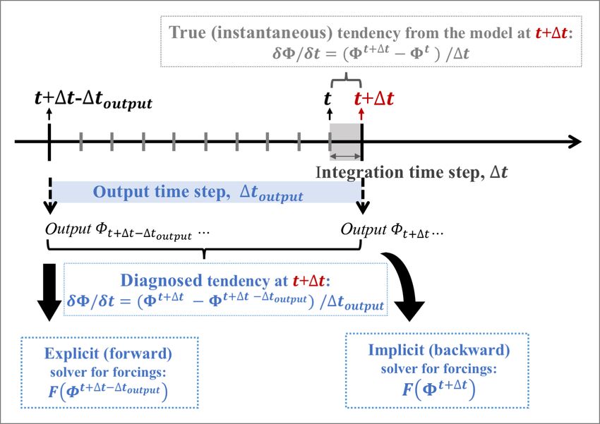
T.-C. Chen et al.: Momentum budget analyses in the WRF (v3.8.1) model 1741
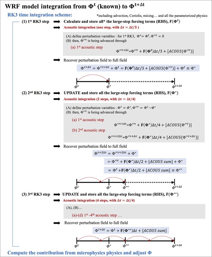
Figure 1. The time integration strategy for advancing a state variable (generalized as 8) in the WRF model based on Skamarock et al. (2008).
In this given example, four acoustic steps are specified for one integration time.
of which uses the same setup but with an increased horizontal is beyond the current scope and will be presented in a subse-
resolution of 2 km, will be discussed in Sect. 4. quent paper.
Figure 2 shows the 48 h evolution of the 99th percentiles
of v and w (hereafter the lowercase indicates that the cal-
culation uses the uncoupled momentum field) and their ten- 3 Methodology and results
dencies. For the 10 km case, the horizontal velocity reaches
its peak in about 20 h, a few hours after the vertical veloc- 3.1 Inline momentum budget analysis
ity reaches its maximum, and then undergoes a weakening.
Both v and w tendencies are maximized at around 15 h. To For the inline budget analysis, all the terms are retrieved di-
understand the evolution of the associated flow dynamics, a rectly from the model for all the integration time steps, and
momentum budget analysis serves as a natural choice. How- therefore they represent the “instantaneous” terms that act
ever, as a preliminary step prior to carrying out such analysis, over the specified short integration time window. For the
we focus only on the technical discussion of the budget anal- large-step forcing, the WRF model accumulates all forcing
ysis methodology. The physical interpretation of the motion terms at the beginning of each RK3 step. To separate them,
we simply take the difference before and after WRF calls the
subroutine for each large-step forcing, store their values sep-
www.geosci-model-dev.net/13/1737/2020/ Geosci. Model Dev., 13, 1737–1761, 2020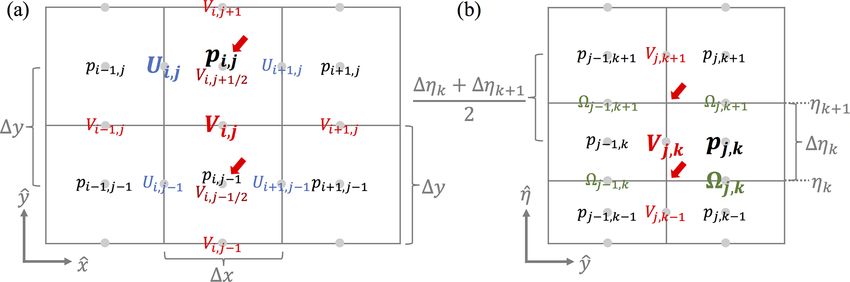
1742                                                   T.-C. Chen et al.: Momentum budget analyses in the WRF (v3.8.1) model

                                                                         where 1t is the model integration time step and 8 repre-
                                                                         sents V or W (coupled momentum; hereafter the momen-
                                                                         tum tendency with capital V or W refers to the lhs term de-
                                                                         rived for the budget analysis). The values of 8 at times t and
                                                                         t + 1t, the latter denoted by superscripts, are termed the cur-
                                                                         rent and predicted states, respectively. Note that while vari-
                                                                         ables of momentum tendencies (specifically named “ru_tend,
                                                                         rv_tend and rw_tend”) can be directly outputted from the
                                                                         WRF model by modifying the registry file, these variables
                                                                         do not necessarily represent the actual momentum changes
                                                                         that consider all the physical (e.g., microphysics, small-step
                                                                         modes) and non-physical processes (e.g., damping) but only
                                                                         the summation of all the large-step forcings.
                                                                            Figures 3 and 4 present the results of the inline budget
                                                                         analysis for horizontal momentum and vertical momentum,
                                                                         respectively, at three selected times (6, 12, and 16 h). To
                                                                         demonstrate the momentum changes in a common physical
                                                                         unit (velocities; meter per second), every term of the flux-
                                                                         form budget equation shown in this paper is divided by the
                                                                         dry-air mass, µd t+1t (so that, for example, the V tendency
                                                                         has a unit of meter per second squared). The magnitude of
                                                                         the V tendency intensifies during this period with local max-
                                                                         ima on the order of 10−4 to 10−3 m s−2 (Fig. 3). Two forc-
Figure 2. Evolutions of the 99 percentiles of (a) horizontal velocity,   ing terms, PGF and COR, are a few times larger than the
v (black; axis on the left), and vertical velocity, w (gray; axis on     ADV term but generally offset each other, making the ADV
the right) in the simulation of slantwise convection. Panel (b) is the   term of comparable importance in determining the tendency.
same as (a) but for their tendencies (black and gray lines for v and w   The CUV term for V tendency is generally small and thus
tendencies, respectively). Solid lines are for the 10 km simulation,     not shown in Fig. 3. The residual, obtained from Eq. (1)
while the dotted ones are for the 2 km case.                             with PV equal to 0, is always smaller than 10−7 m s−2 during
                                                                         the entire 48 h simulation (not shown). To understand how
                                                                         the peak error evolves with time and to avoid reaching mis-
arately, and output only the values at the third RK3 step (the
                                                                         leading conclusions based on one or more outlying values,
total forcing is F (8∗∗ ) 1t as shown in Fig. 1). As for the
                                                                         the evolution of the 99th percentile magnitude of the resid-
contribution of the small-step modes, they are obtained by
                                                                         ual term is shown. Figure 5 shows that it reaches a value of
accumulating over all the small steps in the third RK3 step
                                                                         about 7×10⁻⁹ m s−2 at around 15 h. Recall that the 99th per-
(ACOUS sum shown in Fig. 1). It is worth noting that Eq. (6)
                                                                         centile magnitude of the simulated v tendency has a peak
is a vertically implicit equation that couples with the geopo-
                                                                         of 7 × 10⁻⁴ m s−2 (Fig. 2b). Thus, the relative magnitude
tential tendency equation (Skarmarock et al., 2008; Klemp et
                                                                         of the 99th percentile residual is about 0.001 % of the 99th
al., 2007). A tri-diagonal equation for the vector W (involv-
                                                                         percentile tendency term during the peak intensifying stage.
ing three grid points in the vertical direction) is thus solved
                                                                         Compared to the V tendency, the W tendency exhibits nar-
(Satoh, 2002). This means that W (the scalar at a given grid
                                                                         rower features in the horizontal direction (Fig. 4) with an
point) is not advanced by linear additions in the small-step or
                                                                         overall smaller magnitude in every term. The two largest
acoustic scheme. To ensure the closure of the inline retrieval
                                                                         forcings, PGFBUOY and CUV, usually have opposite signs,
budget, we simply take the total changes that are contributed
                                                                         so their combined effect is on the same order as the ADV and
by the implicit solver in the acoustic scheme as small-step
                                                                         the W tendency term. While the contribution from the upper-
modes of W in the third RK3 step. Note that this way does
                                                                         layer vertical velocity damping is not shown in Fig. 4, it is
not violate the original W equation in Eq. (6). The contribu-
                                                                         included as part of the rhs (PW ) of Eq. (2) when calculat-
tion from these accumulated small-step modes in the V and
                                                                         ing the residual for the inline budget analysis. The residual
W tendency budgets are combined with their large-step PGF
                                                                         in the inline W budget is generally 4 orders of magnitude
and PGFBUOY, respectively, as they share the same mathe-
                                                                         smaller than its tendency term. The 99th percentile residual
matical expressions. Finally, we add the inline calculation for
                                                                         for W budget is about 2 × 10⁻¹⁰ m s−2 , around 0.0003 % of
the tendency term outside of the RK3 integration loop, after
                                                                         the 99th percentile w tendency during the peak intensifying
the microphysics scheme:
                                                                         stage of the convection (not shown).
∂8 t+1t 8t+1t − 8t
       ≡           ,                                              (7)
∂t         1t

Geosci. Model Dev., 13, 1737–1761, 2020                                                   www.geosci-model-dev.net/13/1737/2020/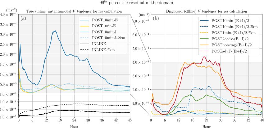
T.-C. Chen et al.: Momentum budget analyses in the WRF (v3.8.1) model                                                                  1743

Figure 3. Inline budget analysis of horizontal momentum, V , with each term extracted directly from the model. In each row, the shading
in each subplot from the left to right shows the term of V tendency, flux-form advection (ADV), horizontal pressure gradient force (PGF),
Coriolis force (COR) (white contours indicate the values exceeding the color bar), PGF+COR, and residual (Eq. 1; PV is 0 and the generally
small curvature term (CUV) is not shown). All terms are divided by µd and thus have units of meters per second squared. The black contours
indicate the horizontal velocity v of 2 and 6 m s−1 (positive and negative values shown in solid and dashed lines, respectively). Each row
from top to bottom illustrates the budget analysis at 6, 12, and 16 h, respectively.

Figure 4. Inline budget analysis of vertical momentum, W , with each term extracted directly from the model. In each row, the shading
in each subplot from the left to right shows the term of W tendency, advection (ADV), net vertical pressure gradient and buoyancy force
(PGFBUOY), curvature (CUV) (white contours indicate the values exceeding the color bar), PGFBUOY + CUV, and residual (Eq. 2; PW is
considered but not shown here). All terms are divided by µd and thus have units of meters per second squared. The black contours indicate the
vertical velocity w of 5 and 15 cm s−1 (positive and negative values shown in solid and dashed lines, respectively). The red (blue) contours
shown in the rightmost column, laid on top of the residual (shading), indicate the small-step components of PGFBUOY with a positive
(negative) value of 3 × 10⁻⁴ m s−2 . Each row from top to bottom illustrates the budget analysis at 6, 12, and 16 h, respectively.

www.geosci-model-dev.net/13/1737/2020/                                                       Geosci. Model Dev., 13, 1737–1761, 2020
1744                                                  T.-C. Chen et al.: Momentum budget analyses in the WRF (v3.8.1) model

3.2     Post-processed momentum budget analyses                      curacy, the output time interval 1toutput needs to be similar
                                                                     to the integration time step 1t.
3.2.1    Key features and methodologies
                                                                     (b) Spatial discretization on the C staggered grid
In contrast to extracting terms directly from the model during
its integration, most of the studies in which the momentum           For computational efficiency and accuracy, WRF utilizes a
budget analysis is conducted use the model output files after        C-grid staggering system (Arakawa and Lamb, 1977). This
the completion of the integration. Note that since the sub-          staggering system is pertinent to the numerical solution for
output time-step information is not available between suc-           spatial derivatives. For most of the spatial derivatives other
cessive outputs, only the large-step forcing terms can be es-        than advection (e.g., the pressure gradient force), the second-
timated in these post-processed budget analyses. Generally,          order finite difference operator is used in the WRF model.
the neglect of the acoustic or small-step modes is expected          For example, the y derivative of variable 8 is calculated us-
to have little impact on the results as the high-frequency           ing the discrete operator:
modes are often considered meteorologically insignificant.           ∂8           1
However, it is mentioned in Klemp et al. (2007) and Ska-                      =        8i,j + 1 ,k − 8i,j − 1 ,k .               (9)
                                                                      ∂y i,j,k 1y             2             2
marock et al. (2008) that the WRF small-step integration
scheme includes not only the acoustic-wave but also some             The index (i, j, k) corresponds to a location with (x, y, η) =
gravity-wave modes, which may not be insignificant. These            (i1x, j 1y, k1η), where 1x, 1y and 1η are the grid lengths
gravity-wave modes form during the small-step integration            in the two horizontal and vertical directions (can be vertically
due to the designated terms that are required for acoustic-          stretched), respectively. The same expression applies for the
wave propagation and “Consequently, in this vertical coordi-         x or the η derivatives. Grid staggering implies that different
nate (i.e., terrain-following hydrostatic pressure coordinate),      variables may be located on different grids, i.e., shifted by
the terms governing the acoustic and gravity wave modes              a half-grid point from the others as illustrated in Fig. 6. De-
are intermingled to the extent that it does not appear feasi-        pending on what variable the spatial derivatives are intended
ble to evaluate any of the gravity wave terms on the large           for, Eq. (9) should be carried out on the corresponding grid,
time steps, even if one desired to do so” (Klemp et al., 2007).      which is not necessarily the same as the 8 grid. For exam-
   Most of the studies did not reveal the complete details           ple, for the V tendency, all the associated forcing terms in-
about how their analysis was done, so we cannot presume              volving the spatial derivatives should be performed on the V
their methodologies and the possible errors. However, a few          grid. More specifically, to calculate the PGF term for the V
simplifications commonly made in the post-processed budget           tendency equation, the term ∂p                    ∂p
                                                                                                    ∂y and the term ∂η in Eq. (1)
analyses may introduce errors that result in deviations from         should be calculated on the V grid but not the pressure grid
the simulated results and thus a significant residual. Below         (p grid). Applying Eq. (9) for ∂p
                                                                                                    ∂y , the V grid with location in-
we revisit the relevant features of the WRF model that should        dices of (i, j − 12 , k) and (i, j + 21 , k) falls exactly on the p grid
be considered and discuss how they might affect the post-            and hence no interpolation is required (red arrows in Fig. 6a).
processed budget if they are ignored. Then, the results are          However, for ∂p ∂η , the pressures on the V grid with indices of
shown for different post-processed budget analyses with dif-
ferent simplifications (Table 1). The aim herein is to identify      (i, j, k − 12 ) and (i, j, k + 12 ) must be obtained (red arrows in
these potential errors hidden in the budget calculation and          Fig. 6b) through linear interpolation using their surrounding
show how severely they affect the resulting interpretation.          closest four pressure values, e.g.,
                                                                     p
(a) Diagnosed tendency                                                V -grid i,j,k+ 12

                                                                         1
                                                                                                                   1ηk+1
                                                                         2   pp-grid(i,j −1,k) + pp-grid(i,j,k)      2
In a post-processed budget analysis, the tendency term of a          =                 1
given variable is approximated by the difference between the                           2    (1ηk + 1ηk+1 )
                                                                                                                       1ηk
value of this variable at two successive output times divided            1
                                                                             pp-grid(i,j −1,k+1) + pp-grid(i,j,k+1)
                                                                         2                                                  2
by the output time interval. Thus, the accuracy may be sen-          +                      1
                                                                                                                                ,       (10)
sitive to the output time interval. The value at the predicted                              2 (1ηk   + 1ηk+1 )
state has a form of                                                  which is weighted by the irregular (stretched) vertical grid-
                                                                     lengths (Fig. 6b).
∂8 t+1t                    8t+1t − 8t+1t−1toutput                       If the C-grid staggering is not considered during the post-
                       ≈                          .           (8)
∂t         diagnosed             1toutput                            processing analysis, i.e., all the variables have been interpo-
                                                                     lated on the universal grids before carrying out the budget
If the output interval is longer than the model integration time     calculation, in addition to the potential errors brought on by
step, the diagnosed tendency would deviate from the model            the interpolation method, the term ∂p∂y , for example, would es-
prediction of the instantaneous tendency. To increase the ac-        sentially involve pressure differences over a larger grid inter-

Geosci. Model Dev., 13, 1737–1761, 2020                                                      www.geosci-model-dev.net/13/1737/2020/
T.-C. Chen et al.: Momentum budget analyses in the WRF (v3.8.1) model 1745
Table 1. A summary of all different approaches for the post-processed horizontal momentum budget analysis that are applied to the model
output after the integration finishes.
Calculated
Order of on C
Form of Output time (vertical; horizontal) Forcing terms diagnosed using staggering
the equation interval advection operators the explicit or implicit method grids
Slantwise convection simulation with a grid length of 10 km and integration time step of 1 min
POST10min-E Flux form 10 min 3; 5 Explicit Yes
POST1min-E Flux form 1 min 3; 5 Explicit Yes
POST10min-I Flux form 10 min 3; 5 Implicit Yes
POST10min-(E+I)/2 Flux form 10 min 3; 5 Average of explicit and implicit Yes
POST2oadv-(E+I)/2 Flux form 10 min 2; 2 Average of explicit and implicit Yes
POSTnonstag-(E+I)/2 Flux form 10 min 3; 5 Average of explicit and implicit No
POSTadvF-(E+I)/2 Advective form 10 min 3; 5 Average of explicit and implicit Yes
Slantwise convection simulation with a grid length of 2 km and integration time step of 10 s
POST10min-I-2km Flux form 10 min 3; 5 Implicit Yes
POST10min-(E+I)/2-2km Flux form 10 min 3; 5 Average of explicit and implicit Yes
POST1min-(E+I)/2-2km Flux form 1 min 3; 5 Average of explicit and implicit Yes
Squall line simulation with a grid length of 250 m and integration time step of 3 s
POST3sec-E Flux form 3s 3; 5 Explicit Yes
Figure 5. Evolution of the 99th percentile of the residual magnitude (meters per second squared) of the horizontal momentum V budget
analysis. For the residual calculation, (a) uses the true V tendency (derived during the integration of the model) and (b) uses the post-
diagnosed V tendency (Eq. 8) as the lhs term. Different colors indicate different post-processed methods for estimating the rhs forcing terms.
The residuals obtained from the inline budget retrieval are in black. Solid and dashed lines are for the 10 km run and 2 km run, respectively.
val of 2×1y instead of 1y, with larger associated truncation nent of the flux-form advection for V momentum in Eq. (3)
errors. as an example, with a fifth-order operator as selected in the
(c) Advection operators
For advection, higher-order operators for finite differencing
are provided as the default WRF setup. Taking the y compo-
www.geosci-model-dev.net/13/1737/2020/ Geosci. Model Dev., 13, 1737–1761, 20201746 T.-C. Chen et al.: Momentum budget analyses in the WRF (v3.8.1) model
Figure 6. (a) Horizontal and (b) vertical C staggering grids for different variables in the WRF model. Note that variables φ and W are
allocated on the same grid as ; µ, α, and q∗ are on grid same as p. The red arrows indicate the grids that would be used to calculate the
second-order spatial derivative term for the V momentum at the V grid (i, j , k).
present simulation, it is written as forcings are updated using a predictor–corrector method in
the second and third RK3 steps. In addition, the W equa-
∂ (V v) 1 5th tion is coupled with the geopotential tendency equation and
− ≈− Vi,j + 1 ,k vi,j + 21 ,k
∂y i,j,k 1y 2 includes a forward-in-time weighting that utilizes predicted
states of the geopotential and temperature in solving the W
5th
−Vi,j − 1 ,k vi,j − 1 ,k
, (11) (Eq. 3.11, 3.12, and 3.19 in Skamarock et al., 2008).
2 2
In numerical analysis for solving ordinary differential
where V and v are the mass-coupled and mass-uncoupled equations, the (explicit) forward Euler method approximates
velocities, respectively: the change of a system from t to t + 1t using the current
1 states (t), while the (implicit) backward Euler method finds
5th 6th the solution using the predicted states (t + 1t):
vi,j 1
− 2 ,k
= v 1
i,j − 2 ,k
− sign V 1
i,j − 2 ,k 60
∂8 t+1t
vi,j +2,k − vi,j −3,k − 5 vi,j +1,k − vi,j −2,k
≈ F 8t forward Euler method,
(12)
∂t
+10 vi,j,k − vi,j −1,k
∂8 t+1t
≈ F 8t+1t backward Euler method.
and (13)
∂t
6th 1 Consistent with this concept, the rhs forcing terms of a bud-
vi,j − 1 ,k
= [37 vi,j,k − vi,j −1,k
2 60 get equation can be estimated using two different instan-
− 8 vi,j +1,k + vi,j −2,k taneous states in analogous ways. However, we emphasize
+ 1 vi,j +2,k + vi,j −3,k ]. that the post-processed budget analysis does not solve the
tendency equation per se but only diagnoses the relation-
The odd-order advection operators include a spatially cen- ship between the two sides of the equation. Note that for
tered even-order operator and an upwind diffusion term. A post-processing analyses, the availability of the data depends
detailed discussion on the advection scheme in the WRF on the output time interval (1toutput ), which is often much
model with different-order operators can be found in Wicker larger than the integration time step (1t). Thus, for the ten-
and Skamarock (2002) and Skamarock et al. (2008). Sim- dency at a given time t + 1t, when applying the forward Eu-
plifying the advection estimation using an operator with an ler method to estimate the associated rhs forcings, the “cur-
order that differs from the numerical setup would contribute rent states” one can use are the most recent prior output at
to errors in the ADV estimation. t + 1t − 1toutput (see Fig. 7):
(d) Forward or backward Euler method ∂8 t+1t
≈ F 8t+1t−1toutput forward Euler method
∂t
Conceptually, the WRF model can be considered more of for post-processing. (14)
a forward scheme, i.e., using the known variables from the
current state to calculate the forcing and then advancing the
variables forward until reaching the prediction time. How- If 1toutput is the same as 1t, Eq. (14) reverts to Eq. (12). If
ever, there are a few implicit components during the integra- 1toutput is much larger than 1t, the backward Euler method
tion. For example, as discussed in Sect. 2.1, the large-step using predicted states at t + 1t may better estimate the true
Geosci. Model Dev., 13, 1737–1761, 2020 www.geosci-model-dev.net/13/1737/2020/T.-C. Chen et al.: Momentum budget analyses in the WRF (v3.8.1) model 1747
1
first multiplied by a factor of µd and V is rewritten as µd v:
1 ∂(µd v) 1
= − ∇ · (µd vv)
µd ∂t µd
| {z } | {z }
V tendency advection
ADV
1 ∂p α ∂p ∂φ
+ −α −
µ ∂y αd ∂η ∂y
|d {z }
horizontal pressure gradient force
PGF
1 1 vW 1
− fU− + PV . (16)
Figure 7. Schematic plot showing the explicit (forward) and im- µd µ r µ
| {z } | d {z e } | d{z }
plicit (backward) solvers for the rhs forcing terms, as well as the
Coriolis curvature remaining
diagnosed and the true (calculated inline during the integration of
the model) lhs tendency term defined in this study. COR CUV (parameterized)
physics
Then, by adding the mass continuity equation in WRF (mul-
tiplied by a factor of µvd ):
model forcing terms as they are calculated using variables
at a closer time to the real integration window in the model
v ∂µd
(Fig. 7). + ∇ · (µd v) = 0
µd ∂t
The above two diagnostic methods estimate the forcing
terms using instantaneous states. However, as mentioned in
Sect. 3.2.1(a), the diagnosed lhs tendency depends on two to the rhs of Eq. (16), we obtain
successive model output times. Thus, an average between
forcings diagnosed explicitly and implicitly are often con-
sidered. For a post-processed analysis, this translates into es- 1 ∂(µd v) v ∂µd v 1
timating the forcings using both predicted states and the most = + ∇ · (µd v) − ∇ · (µd vv)
µd ∂t µd ∂t µd µd
recent prior available current states: | {z } | {z }
V tendency advection
ADV
1 ∂p α ∂p ∂φ 1
+ −α − − fU
µ ∂y αd ∂η ∂y µd
∂8 t+1t 1 | d {z } | {z }
F 8t+1t−1toutput + F 8t+1t . (15)
≈ horizontal pressure gradient force Coriolis
∂t diagnosed 2
PGF COR
1 vW 1
− + PV .
µ r µ
| d {z e } | d{z }
curvature remaining
(e) Flux or advective form of equation CUV (parameterized)
physics
(17)
While the momentum equations solved in the WRF model
are in flux form, their corresponding advective forms can be
derived and are often used for post-processed budget analy- Moving the first term on the rhs of Eq. (17) to the lhs, the sec-
ses for convenience. To derive the advective form, the flux- ond rhs term can be combined with the flux-form advection
form V momentum equation (Eq. 1 excluding residual) is using the vector identity ∇ · (µd v) = µd (∇ · v) + v · (∇µd ).
www.geosci-model-dev.net/13/1737/2020/ Geosci. Model Dev., 13, 1737–1761, 20201748 T.-C. Chen et al.: Momentum budget analyses in the WRF (v3.8.1) model
Then, the advective form of the horizontal momentum equa- post-processed budget. These inherent errors result in a small
tion is obtained as residual term with a general order of 10−5 m s−2 , 1 to 2 or-
der(s) smaller than the maximum V tendency. In terms of
∂v local maxima, the 99th percentile magnitude of the residual
= |−v{z
· ∇v} obtained in POST1min-E gives a relative magnitude of about
∂t
|{z}
advection ADV 7 % of the 99th percentile v tendency during the peak intensi-
v tendency fying stage of the convection at around 15 h (Figs. 2b and 5).
in advective form
in advective form Although reducing the model output interval to be close to
1
∂p α ∂p ∂φ
the integration time step helps to balance the budget without
+ −α − the need for inline diagnoses, it is computationally expensive
µ ∂y αd ∂η ∂y
| d {z } especially for large, data-intensive simulations.
horizontal pressure gradient force Given that computational cost is often a major consider-
PGF ation, we also test whether the implicit or backward Euler
method (POST10min-I) can improve the estimation of in-
1 1 vW
− fU− stantaneous forcing terms relative to the explicit method for
µd µ r
| {z } | d {z e } the same 10 min output data (POST10min-E). POST10min-I
Coriolis curvature follows the same strategy as POST10min-E except that all
COR the rhs terms, following Eq. (13), are diagnosed with the
CUV
predicted states instead of the previous output states. As de-
1 picted in Fig. 10, POST10min-I does indeed better capture
+ PV . (18)
µd the true model estimated forcing values as errors in all the
| {z }
rhs forcing terms diminish greatly to an accuracy similar to
remaining
POST1min-E. However, as these forcings are calculated at
(parameterized)
a given instant, the imbalance of the budget would remain
physics
if the diagnosed tendency term is not calculated instanta-
3.2.2 Results of horizontal momentum budget neously (the second column from the right in Fig. 10). There-
fore, if budget analysis at an instant of time is desired, we rec-
Table 1 summarizes all the post-processed budget analyses ommend adding the tendency calculation within the model as
tested in this study. In the present section, we first present a standard output and diagnosing the forcing terms implicitly,
the results one by one, and then a qualitative intercompari- which yields a residual term on a similar order to the one ob-
son among them and the inline retrieval method is discussed. tained in POST1min-E (the rightmost column in Fig. 10 and
The first post-processed method (POST10min-E) for V bud- Fig. 5a).
get follows all the approaches in the model as closely as pos- For the more common situation, the post-processed anal-
sible using the 10 min output data. The flux-form equation, yses diagnose rhs terms using two successive outputs over
C staggering grids, and the same orders of advection oper- an output time interval, i.e., taking the averages of the ex-
ators as the experimental setup are used. The diagnosis of plicitly and implicitly calculated forcings using Eq. (15) on
the large-step forcing is applied directly to the model out- the 10 min output (POST10min-(E+I)/2). Comparing the av-
puts on η levels using the explicit or forward Euler method eraged rhs forcings with the analogously diagnosed lhs mo-
as shown in Eq. (14). The diagnosed forcing terms are com- mentum tendency (Eq. 8) gives a small residual to a similar
pared with their corresponding true values from the inline accuracy level as POST1min-E and POST10min-I (the right-
retrieval (Fig. 8). Errors smaller than, but on the same order most column in Figs. 11 and 5b).
of 10−4 m s−2 as the V tendency, are observed in all terms We now investigate the impact of other common simpli-
including the diagnosed tendency term. These errors grow in fications on top of the reference experiment, POST10min-
magnitude and areal coverage with the growth of the distur- (E+I)/2. The first such simplification is to approximate
bance. Aside from COR, the absolute errors in the tendency, the flux-form advection term using the second-order oper-
ADV and PGF can exceed 6 × 10⁻⁴ m s−2 , the former two ator (Eq. 9) for both vertical and horizontal components
of which are more than 50 % of the magnitude of their true (POST2oadv-(E+I)/2) instead of the third- and fifth-order op-
(instantaneous) values locally. erators as used in the model setup. In our simulation, such
The second post-processed analysis (POST1min-E) is inconsistency of advection operators introduced errors in the
done following the same approach but applied to the 1 min ADV term with a maximum value > 3 × 10⁻⁴ m s−2 , more
(same as the integration time step for this simulation) out- than 50 % of its true magnitude along the slantwise convec-
put data, and the results show strongly reduced errors in all tive band (Fig. 12). Next, we repeated POST10min-(E+I)/2
terms (Fig. 9). The errors that remain are mostly in the PGF but the calculation is applied after all the model output vari-
term and likely stem from the fact that the small-step modes ables have been interpolated to the universal or un-staggered
and the RK3 integration scheme are not considered in the grid (pressure grid) (POSTnonstag-(E+I)/2). This is a com-
Geosci. Model Dev., 13, 1737–1761, 2020 www.geosci-model-dev.net/13/1737/2020/T.-C. Chen et al.: Momentum budget analyses in the WRF (v3.8.1) model 1749 Figure 8. The difference between the post-processed (POST10min-E; with an explicit or forward method on 10 min output) and inline budget analysis for the horizontal momentum, V . All terms have been divided by µd and thus have a uniform unit of meters per second squared. In each row, from left to right indicates the difference for V tendency, ADV, PGF, and COR. The rightmost column indicates the residual term obtained in the post-processed budget analysis. Each row from top to bottom shows the results at 6, 12, and 16 h, respectively. Figure 9. Same as Fig. 8, but the post-processed budget analysis is applied to the data with an output time interval of 1 min (POST1min-E). mon way to post-process model output data for plotting pur- tendency term over a wide area and is reaching 100 % over poses. As mentioned earlier, this approach would reduce the the band head). accuracy when solving the spatial differential terms, and in- Finally, a different format of the V equation, the advec- deed, the results do indicate significant errors over a large tive form, is used for post-processed analysis (POSTadvF- area in both ADV and PGF (Fig. 13). Their combined er- (E+I)/2). Mathematically, the flux-from momentum equation rors result in widespread residual values > 3 × 10⁻⁵ m s−2 can be rewritten in the advective form without making any even over the area where the tendency term is smaller than additional approximation, only with the aid of the conser- 1 × 10⁻⁴ m s−2 (error is at least of 30 % magnitude of the vation law of dry-air mass in the WRF model as shown in www.geosci-model-dev.net/13/1737/2020/ Geosci. Model Dev., 13, 1737–1761, 2020
1750                                                 T.-C. Chen et al.: Momentum budget analyses in the WRF (v3.8.1) model

Figure 10. Same as Fig. 8, but the post-processed rhs terms are diagnosed using the implicit or backward method (POST10min-I) and an
extra column is added on the rightmost showing the residual from the true tendency (i.e., the instantaneous value obtained from the model).

Figure 11. Same as Fig. 8, but the forcing terms diagnosed in the post-processed budget analysis are the averages of explicit and implicit
methods (POST10min-(E+I)/2). To represent the same time window as the post-processed analysis, the inline budget results used here for
the difference calculation are the 10 min averages (corresponding to the output interval) instead of the instantaneous values.

Eqs. (16)–(18). However, during the interchange of the ex-              lated v tendency) in our study. The summation of the ten-
pression for the tendency and advection terms, truncation er-           dency term and advection term in these two forms of the
rors may be introduced. We reiterate that the tendency term             momentum equation should be mathematically identical, so
in the advective form is not equivalent to the one in the flux          we would expect to see a small difference in the advection
form divided by µd ; however, calculation suggests that they            term as in the tendency term. However, we find that the
are approximately equal, i.e.,                                          advection term in the advective form has a strong positive
1 ∂(µd v) ∂v                                                            bias compared to that in the flux form (Fig. 14). The resid-
         ≈    ,                                                         ual term in the POSTadvF-(E+I)/2 is thus negatively biased
µd ∂t      ∂t
                                                                        over the entire convective band with a magnitude exceeding
with a maximum error that is on the order of 10−7 ∼                     1.2 × 10⁻⁴ m s−2 (reaching 100 % error near the upper half
10−8 m s−2 (3 orders of magnitude smaller than the simu-

Geosci. Model Dev., 13, 1737–1761, 2020                                                    www.geosci-model-dev.net/13/1737/2020/
T.-C. Chen et al.: Momentum budget analyses in the WRF (v3.8.1) model 1751
Figure 12. Same as Fig. 11, but the post-processed analysis uses a second-order operator for advection calculation (POST2oadv-(E+I)/2).
of the convective band). If the residual is neglected or not similar results although the relative magnitudes of such cho-
shown, authors and/or readers may falsely consider the ad- sen residuals among the three post-processing methods with
vection process to be the dominant term governing the evo- simplifications (POST2oadv-(E+I)/2, POSTnonstag-(E+I)/2,
lution of the slantwise updraft. and POSTadvF-(E+I)/2) vary due to their different error dis-
A quantitative comparison of the 99th percentile of the tributions.
magnitude of the residual term in the domain (excluding the
boundaries) among different analysis methods is shown in 3.2.3 Results of vertical momentum budget
Fig. 5. The residuals between the instantaneously diagnosed
forcings and the true model tendency term (calculated in- For the W equation, the closure of the post-processed budget
line) are shown in Fig. 5a while the ones between the aver- appears not to be practicable even when the output time in-
aged forcings of two consecutive outputs and the diagnosed terval is reduced to the integration time step (Fig. 15). One
tendency term are shown in Fig. 5b. The evolution of the partial reason is that the spatially noisy small-step modes, ne-
99th percentile residual shows generally larger magnitudes glected in the offline budget analysis, are surprisingly large
when the momentum tendency is larger (Fig. 2b), suggesting with a general order of 10−4 m s−2 over the growing band,
that these errors may amplify in stronger convection cases. which is 1 order of magnitude larger than the W tendency
While the post-processed budget analysis in POST1min- (see the blue and red contours overlapped on the residual
E, POST10min-I, and POST10min-(E+I)/2 can achieve a subplots in Fig. 4). These high-frequency modes not only in-
relatively small 99th percentile residual (peak at ∼ 5 × clude vertically propagating sound waves but also some grav-
10−5 m s−2 , or about 7 % of the concurrent 99th percentile v ity wave modes (Klemp et al., 2007). Furthermore, as indi-
tendency), the inline budget analysis always gives a much cated in Eq. (6) and mentioned in Sect. 3.1, the W equation
smaller magnitude (< 10−8 m s−2 , or 0.001 % of the ten- solved in the WRF model is implicit, coupled with geopoten-
dency, during the entire simulation). Figure 5 also shows that tial tendency equation and includes a forward-in-time aver-
any simplification that is inconsistent with the model solver aging operator that is applied to the small-step modes:
can severely degrade the accuracy of the post-processed
budget analysis. Both POSTnonstag-(E+I)/2 and POSTadvF- τ 1+β 1−β
(ACOUS) = (ACOUS)τ +1τ + (ACOUS)τ ,
(E+I)/2 can lead to a 99th percentile of the residual magni- 2 2
tude peaking at around 4 × 10⁻⁴ m s−2 or more, which cor-
where β is a user-specified parameter and 1τ indicates the
responds to > 50 % of their concurrent 99th percentile sim-
small time step in the acoustic scheme. This means that the
ulated v tendency, respectively. Generally, a higher relative τ
small-step modes at a current small step, (ACOUS) , are cal-
magnitude of residual to v tendency is reached if the max-
culated using information (e.g., geopotential, potential tem-
imum instead of the 99th percentile is examined (despite
perature and density) at the forecast time τ +1τ (see Eq. 3.11
larger fluctuation with time). We also examined the 95th per-
and 3.12 in Skamarock et al., 2008). All these components
centile of the residual magnitude and obtained qualitatively
are not feasible for an offline budget calculation.
www.geosci-model-dev.net/13/1737/2020/ Geosci. Model Dev., 13, 1737–1761, 20201752 T.-C. Chen et al.: Momentum budget analyses in the WRF (v3.8.1) model Figure 13. Same as Fig. 11, but the post-processed analysis does not consider C staggering grids (POSTnonstag-(E+I)/2). Figure 14. Same as Fig. 11, but the post-processed analysis is applied using the advective-form equation (POSTadvF-(E+I)/2). The application of POST1min-E for the W tendency (not shown). However, this large-step forcing term adjusts shows that this method accurately estimates most of the pro- rapidly, sometime even with a sign change, from step to step cesses, but large errors > 2 × 10⁻³ m s−2 remain in the PGF- within the RK3 integration. Although it is feasible to esti- BUOY term resulting in a widespread residual that reaches mate F (8t ) via post-processing, it is however impossible to the same magnitude of the peak W tendency term (Fig. 15). retrieve F (8∗∗ ) in Eq. (4), leading to the poor estimation of The fact that these errors exceed the small-step modes (con- vertical pressure gradient and buoyancy force in the W bud- tributing to PGFBUOY) suggests that such imbalance does get. This result also suggests that the budget closure for ver- not solely come from the neglect of the small-step modes. tical velocity is difficult by nature due to its rapid variation A close comparison of the post-processed and the inline on small scales. PGFBUOY shows that our estimation is close to the inline value to an accuracy of at least three significant figures at the first RK3 step before the acoustic contribution is considered Geosci. Model Dev., 13, 1737–1761, 2020 www.geosci-model-dev.net/13/1737/2020/
You can also read