Mixing at the extratropical tropopause as characterized by collocated airborne H2O and O3 lidar observations - Recent
←
→
Page content transcription
If your browser does not render page correctly, please read the page content below
Atmos. Chem. Phys., 21, 5217–5234, 2021
https://doi.org/10.5194/acp-21-5217-2021
© Author(s) 2021. This work is distributed under
the Creative Commons Attribution 4.0 License.

Mixing at the extratropical tropopause as characterized by
collocated airborne H2O and O3 lidar observations
Andreas Schäfler, Andreas Fix, and Martin Wirth
Deutsches Zentrum für Luft- und Raumfahrt, Institut für Physik der Atmosphäre, Oberpfaffenhofen, Germany

Correspondence: Andreas Schäfler (andreas.schaefler@dlr.de)

Received: 18 October 2020 – Discussion started: 26 October 2020
Revised: 16 February 2021 – Accepted: 18 February 2021 – Published: 1 April 2021

Abstract. The composition of the extratropical transition           pacted the ExTL above and below the jet stream which is a
layer (ExTL), which is the transition zone between the strato-      confirmation of the well-established concept of turbulence-
sphere and the troposphere in the midlatitudes, largely de-         induced mixing in strong wind shear regions. At the level of
pends on dynamical processes fostering the exchange of air          maximum winds reduced mixing is reflected in jumps in T–T
masses. The Wave-driven ISentropic Exchange (WISE) field            space that occurred over small horizontal distances along the
campaign in 2017 aimed for a better characterization of the         cross section. For a better understanding of the dynamical
ExTL in relation to the dynamic situation. This study inves-        and chemical discontinuities at the tropopause, the lidar data
tigates the potential of the first-ever collocated airborne lidar   are illustrated in isentropic coordinates. The strongest gra-
observations of ozone (O3 ) and water vapor (H2 O) across           dients of H2 O and O3 are found to be better represented by
the tropopause to depict the complex trace gas distributions        a potential vorticity-gradient-based tropopause compared to
and mixing in the ExTL. A case study of a perpendicu-               traditional dynamical tropopause definitions using constant
lar jet stream crossing with a coinciding strongly sloping          potential vorticity values. The presented 2D lidar data are
tropopause is presented that was observed during a research         considered to be of relevance for the investigation of fur-
flight over the North Atlantic on 1 October 2017.                   ther meteorological situations leading to mixing across the
   The collocated and range-resolved lidar data that are ap-        tropopause and for future validation of chemistry and numer-
plied to established tracer–tracer (T–T) space diagnostics          ical weather prediction models.
prove to be suitable to identify the ExTL and to reveal dis-
tinct mixing regimes that enabled a subdivision of mixed
and tropospheric air. A back projection of this informa-
tion to geometrical space shows remarkably coherent struc-          1   Introduction
tures of these air mass classes along the cross section. This
represents the first almost complete observation-based two-         The extratropical transition layer (ExTL) is a subregion of
dimensional (2D) illustration of the shape and composition of       the extratropical upper troposphere and lower stratosphere
the ExTL and a confirmation of established conceptual mod-          (ExUTLS) which is relevant both for climate (Riese et al.,
els. The trace gas distributions that represent typical H2 O        2012) and weather (Gray et al., 2014). Radiatively active
and O3 values for the season reveal tropospheric transport          trace gases, like ozone (O3 ) and water vapor (H2 O), pro-
pathways from the tropics and extratropics that have influ-         vide significant vertical gradients across the ExTL, and the
enced the ExTL. Although the combined view of T–T and               tropopause therein, that impact the Earth’s radiation bud-
geometrical space does not inform about the process, loca-          get. The transition from the troposphere to the stratosphere
tion and time of the mixing event, it gives insight into the        can be abrupt or more uniform in cases when the ExTL is
formation and interpretation of mixing lines. A mixing fac-         strongly impacted by two-way stratosphere–troposphere ex-
tor diagnostic and a consideration of data subsets show that        change (STE) processes. Depending on their lifetime, trace
recent quasi-instantaneous isentropic mixing processes im-          gases reveal a footprint of the mixing processes in their La-
                                                                    grangian history, typically as an intermediate chemical char-

Published by Copernicus Publications on behalf of the European Geosciences Union.
5218                                                              A. Schäfler et al.: Mixing at the extratropical tropopause

acteristic with both tropospheric and stratospheric influence,    undisturbed background to explore the average composition
highlighting irreversible and bidirectional transport between     and extent of the ExTL (see summary in Gettelman et al.,
the spheres (Gettelman et al., 2011). These mixing processes      2011). Many of these climatological studies made use of data
strongly depend on the dynamical situation. For a better un-      from multiple research flights or multiple campaigns or used
derstanding of the role of multiscale dynamical processes on      satellite data. In situ observations of chemical species on
the composition of the ExTL in the midlatitudes, the Wave-        board commercial aircraft (e.g., Brenninkmeijer et al., 2007)
driven ISentropic Exchange (WISE) field campaign (Kunkel          are restricted to the flight routes and the altitude range of the
et al., 2019) was conducted over the North Atlantic Ocean         aircraft and provide only a limited number of vertical profiles
in autumn 2017. The HALO (High Altitude LOng range)               during start and landing (Zahn et al., 2014). The use of satel-
research aircraft performed in situ and remote sensing mea-       lite observations guarantees a high temporal resolution and
surements of various trace gases in the ExTL from turbulence      global coverage but, however, is limited in vertical resolution
to synoptic scales in a variety of meteorological situations.     (about 1–3 km in the UTLS) and rather high measurement
   Mixing in the extratropics is often related to upper-level     uncertainty in the tropopause region (Hegglin et al., 2008,
frontal zone–jet-stream systems (Keyser and Shapiro, 1986;        2009). Aircraft in situ data obtained during research cam-
Lang and Martin, 2012) that are characterized by isentropic       paigns are highly accurate and temporally resolved, however,
surfaces that cross the sloped tropopause (Holton et al., 1995;   with limited spatial and temporal coverage.
Stohl et al., 2003). The highly variable midlatitude flow is         Several case studies, typically using repeated in situ flight
largely affected by baroclinic cyclones that develop from dis-    legs at different altitudes to provide a certain altitude reso-
turbances in the jet stream and cause a strong distortion of      lution, showed a strong influence of the synoptic situation
the tropopause through the redistribution of tropospheric and     on the interplay of dynamics and chemistry (e.g., Pan et
stratospheric air masses. Intrusions of stratospheric air into    al., 2007; Vogel et al., 2011; Konopka and Pan, 2012). Pan
the troposphere are connected to jet streams and cyclones         et al. (2007) contrast two different dynamical conditions, a
and represent areas of irreversible mixing of tropospheric        strong jet stream with a complex tropopause fold structure
and stratospheric air due to filamentation (Danielsen, 1968;      and a flat tropopause situation, and found a correlation be-
Danielsen et al., 1987) and roll-up of intrusions (Appen-         tween the sharpness of the chemical and thermal transitions
zeller et al., 1996). Strong wind shear above and below the       with minimal mixing in the flat tropopause situation. Mixed
jet stream maximum results in clear air turbulence fostering      air masses dominated on the cyclonic jet stream side in an
the exchange between stratosphere and troposphere (Shapiro,       area where the dynamical and thermal tropopause altitudes
1976, 1980). Recently, Spreitzer et al. (2019) have shown         were separated. Konopka and Pan (2012) used in situ obser-
the importance of turbulence in upper-level frontal zone–jet-     vations in combination with a trajectory model to demon-
stream systems and tropopause folds for midlatitude dynam-        strate that large parts of the ExTL near a jet stream are
ics. Beside turbulence, a variety of other non-conservative       formed on timescales of a few days, especially in the lower
diabatic processes occur near jet streams and cyclones that       part of the jet stream. A combined approach of in situ data in
foster cross-isentropic mixing, e.g., cloud diabatic processes    geometrical and T–T space was used to locate mixed, strato-
in convective or large-scale clouds (Gray, 2003; Wernli and       spheric and tropospheric air masses along selected flight legs
Bourqui, 2000) or radiative processes related to vertical H2 O    crossing the ExTL horizontally and vertically (Pan et al.,
gradients or clouds (Zierl and Wirth, 1997). Additionally,        2006, 2007; Vogel et al., 2011; Konopka and Pan, 2012).
thunderstorms were shown to impact the ExTL composition           However, a detailed attribution of mixing lines to locations
(e.g., Huntrieser et al., 2016; Pan et al., 2014a), often being   in geometrical space and an isentropic investigation was so
triggered by large-scale weather systems. The spatiotempo-        far limited by the reduced information content of staggered
ral diversity of the flow and the complex life of cyclones re-    in situ legs.
sult in a large variety of mixing and exchange processes that        The interrelation of chemical and dynamical discontinu-
were found through case studies and climatologies (Sprenger       ities at the tropopause is of central interest to understand
and Wernli, 2003; Škerlak et al., 2014; Reutter et al., 2015;     trace gas distributions and their relation to transport and
Boothe and Homeyer, 2017) and explain the complexity that         mixing processes. However, the analysis of the structure
ExTL observations have shown in terms of their chemical           and location of the ExTL depends on the definition of the
characteristics.                                                  tropopause (e.g., Pan et al., 2004). In the vertical the ExTL
   Mixed air masses can be identified by relationships be-        is centered on the thermal tropopause, while the dynam-
tween long-lived chemical trace gases (Hintsa et al., 1998,       ical tropopause (using a 2 potential vorticity, PV, unit –
Fischer et al., 2000; Hoor et al., 2002; Zahn and Bren-           1 PVU = 10−6 K m2 kg−1 s−1 – definition) marks the bottom
ninkmeijer, 2003; Pan et al., 2004). This correlation of tro-     of the ExTL. Near the extratropical jet stream where the ther-
pospheric and stratospheric tracers with opposing behavior        mal tropopause typically features a large break in altitude, the
(tracer–tracer or T–T correlation, explained in more detail in    dynamical tropopause runs almost vertical across isentropes.
Sect. 2.2), e.g., of O3 and H2 O, was used to separate mixed      Kunz et al. (2011b) found better consistency of isentropic
air masses of intermediate chemical characteristics from the      trace gas gradients with a PV-gradient tropopause (Kunz et

Atmos. Chem. Phys., 21, 5217–5234, 2021                                             https://doi.org/10.5194/acp-21-5217-2021

A. Schäfler et al.: Mixing at the extratropical tropopause                                                                 5219

al., 2011a) compared to fixed PV thresholds defining the dy-         – Can the O3 and H2 O observations for a range of isen-
namical tropopause. However, for an instantaneous latitudi-            tropic levels at the midlatitude tropopause be used for
nal cross section, they could only show that this holds for            an improved localization of the chemical and dynamical
simulated trace gas data.                                              discontinuity between stratosphere and troposphere?
    Two-dimensional (2D) profiles from active and passive
remote sensing instruments on board research aircraft can            – How can mixing lines be interpreted correctly? What
fill the observational gap between airborne in situ and satel-         can we learn on the formation of mixing lines for differ-
lite measurements. Passive airborne limb sounders enable re-           ent data subsets along the cross section?
trieving vertical profiles of a multitude of trace gas species
                                                                    This paper will describe the DIAL O3 and H2 O lidar ob-
(Ungermann et al., 2013). Limb sounders provide a good
                                                                 servations in Sect. 2.1 and their combined application to es-
along track (∼ 3 km) and vertical resolution (200 to 300 m
                                                                 tablished T–T diagnostics in Sect. 2.2. The synoptic situa-
depending on the observed altitude) to resolve tropopause-
                                                                 tion of a textbook-like transect of a zonal extratropical jet
based gradients. However, the low resolution along their line-
                                                                 stream over the North Atlantic Ocean on 1 October 2017 is
of-sight requires homogeneity in viewing direction as gradi-
                                                                 explained in Sect. 3.1. In Sect. 3.2 to 3.4 the lidar data are
ents can cause artifacts in the trace gas profiles. Woiwode
                                                                 presented along cross sections, in T–T space and in combined
et al. (2019) illustrate the applicability of the linear limb-
                                                                 view, respectively. The interrelation of chemical and dynami-
imaging GLORIA (Gimballed Limb Observer for Radiance
                                                                 cal discontinuities at the midlatitude tropopause is described
Imaging of the Atmosphere) to observe the fine structure of
                                                                 in Sect. 3.5. A discussion of the results and conclusion is
a tropopause fold. In contrast, active remote sensing with an
                                                                 given in Sect. 4.
airborne differential absorption lidar (DIAL) offers both a
high horizontal and vertical resolution directly beneath the
aircraft. Early pioneering studies demonstrated the signifi-     2     Data and methods
cance of range-resolved profiles of O3 (Browell et al., 1987)
and of H2 O (Ehret et al., 1999) to characterize mesoscale       2.1    Lidar observations on board HALO
tropopause folds. The benefit of using simultaneous lidar
measurements of H2 O and O3 was emphasized by Kooi et            During the WISE campaign, the German research aircraft
al. (2008) showing observations in the tropical troposphere.     HALO (Krautstrunk and Giez, 2012) was equipped with
However, the DIAL they used was not capable of accurately        the WAter vapor differential absorption Lidar Experiment in
measuring the low H2 O mixing ratios occurring in the strato-    Space (WALES), which was originally designed as a four-
sphere (Browell et al., 1998). Pan et al. (2006) combined li-    wavelength H2 O DIAL operating at 935 nm (Wirth et al.,
dar O3 cross sections with in situ data to investigate mixing    2009). In the past, WALES was characterized by and ap-
in the ExTL.                                                     plied in multiple campaigns focusing on various topics rang-
    Recently, collocated profile observations of H2 O and O3     ing from atmospheric dynamics (e.g., Schäfler and Harnisch,
across the extratropical tropopause from a single aircraft to    2015; Schäfler et al., 2018), moisture transport (e.g., Schäfler
investigate the structure of the ExTL became possible (Fix et    et al., 2010; Kiemle et al., 2011) and cloud microphysics
al., 2019). This methodology thus provides new insights into     (Urbanek et al., 2017) to UTLS investigations (Trickl et al.,
the 2D structure of the ExTL and the chemical and dynamical      2016). In 2012, the system was extended by an optional O3
discontinuity therein in order to verify past concepts and add   DIAL capability (Fix et al., 2019) to be able to measure col-
new details to our current knowledge (see review article by      located profiles of O3 and H2 O. During the Polar Strato-
Gettelman at al., 2011). This study therefore makes use of       sphere in a Changing Climate (POLSTRACC; Oelhaf et al.,
these unique observations to address the following questions.    2019) campaign in 2016, this capability was used for the first
                                                                 time but in a zenith-pointing mode for stratospheric observa-
  – Is the precision of O3 and H2 O lidar observations suf-
                                                                 tions. However, during WISE the lidar was exclusively mea-
    ficient to determine the ExTL using established T–T di-
                                                                 suring nadir.
    agnostics? Can the 2D structure of the ExTL along an
                                                                    The measurement principle of the DIAL is based on the
    extratropical jet stream crossing be depicted by a back
                                                                 differential absorption of laser pulses at two or more wave-
    projection of diagnostics from T–T space to geometrical
                                                                 lengths. The spectrally close wavelengths are selected such
    space?
                                                                 that absorption and scattering properties on their way through
  – Does this combined view reveal distinct mixing regimes       the atmosphere only differ with respect to absorption by the
    along the cross section that provide information on the      trace gas of interest, i.e., O3 and H2 O. Accordingly, the sys-
    complex chemical structure and mixing state of the           tem creates two wavelengths for H2 O DIAL in the absorp-
    ExTL? How do they relate to the dynamical situation          tion band at 935 nm and two wavelengths for O3 DIAL at
    and what do they tell about the preceding transport of       305 and 315 nm. For both pairs of wavelengths, one wave-
    the observed air masses? How representative is the pre-      length provides a strong absorption depending on the trace
    sented case study?                                           gas concentration, while the other is absorbed only weakly,

https://doi.org/10.5194/acp-21-5217-2021                                           Atmos. Chem. Phys., 21, 5217–5234, 2021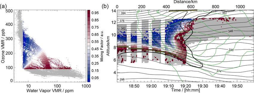
5220                                                               A. Schäfler et al.: Mixing at the extratropical tropopause

resulting in a stronger backscatter signal. From the ratio of      plained by the rather weak variability in the tropospheric and
both signals as a function of the time taken to pass through       stratospheric trace gas concentrations that are connected by
the atmosphere and the knowledge about the exact absorption        the mixing lines on timescales of individual research cam-
characteristics, a range-dependent determination of O3 and         paigns or seasons (Hegglin et al., 2009). This allowed a sta-
H2 O number densities in the illuminated volume becomes            tistical investigation of the ExTL depth and composition, al-
possible. To reduce statistical noise in the signals, these are    though the individual flights may have covered various dy-
temporally averaged over 24 s, which corresponds to a 5.6 km       namical situations and air masses of different origins (e.g.,
distance between neighboring profiles. In this study, O3 and       Pan et al., 2004; Hoor et al., 2004; Hegglin et al., 2009).
H2 O is determined every 15 m in the vertical although it has         A prerequisite for the T–T method is that the distributions
to be mentioned that the effective vertical resolution of the      are controlled by transport processes, i.e., that the lifetime
data is 500 m (full width at half maximum, FWHM, of the            of the trace gases used is longer than the timescale of trans-
averaging kernel) and exactly the same for O3 and H2 O. The        port and mixing at the tropopause, which is in the order of
observed number density from the DIAL is converted to vol-         weeks. In this study O3 –H2 O correlations are applied. Pan
ume mixing ratios (VMRs) using profiles of temperature and         et al. (2007) note that H2 O is a suitable tropospheric tracer
pressure typically taken from numerical weather prediction         despite the fact that it is not perfectly long-lived as phase
models (see Sect. 2.3). For a detailed characterization and        changes may cause non-conservation of the gas-phase H2 O
validation of the instrument, the interested reader is referred    concentration. As discussed in Hegglin et al. (2009), the ex-
to Wirth et al. (2009) and Fix et al. (2019). Note that through-   ponential decrease in H2 O across the tropopause makes it
out the present study H2 O VMR is given as parts per million       a very useful source of information about transport into the
(ppm) which is equivalent to 10−6 mol mol−1 or µmol mol−1 ,        stratosphere as even small amounts of H2 O become visible
and O3 VMR uses parts per billion (ppb) which is equivalent        as a signature of increased H2 O. In the stratosphere, methane
to 10−9 mol mol−1 or nmol mol−1 .                                  oxidation can produce H2 O which is, however, rather small
                                                                   in the lower stratosphere (LS) and therefore often neglected
2.2    Tracer–tracer correlation                                   (Pan et al., 2014b). Due to the large dynamic range of H2 O
                                                                   of 4 orders of magnitude from the troposphere to the strato-
One of the key methods that is applied here is the presenta-       sphere, T–T depictions of the H2 O data are displayed in loga-
tion of the lidar data in T–T space, which is a well-established   rithmic scaling to be able to distinguish the mixing lines (e.g.,
method to investigate the chemical transition in the ExTL          Hegglin et al., 2009; Tilmes et al., 2010), which are typically
(Hintsa et al., 1998; Fischer et al., 2000; Zahn and Bren-         curved in log-linear T–T diagrams, more easily.
ninkmeijer, 2003). When the concentration of a trace gas              Stratospheric and tropospheric background distributions
with its main sources in the stratosphere is displayed in re-      are usually selected in T–T space by defining case-dependent
lation to the concentration of another trace gas with its main     threshold concentrations. One method uses thresholds, e.g.,
sources in the troposphere, in the idealized situation of no       H2 O ≤ 5 ppm to select the stratospheric branch and O3 ≤
mixing, this T–T correlation method shows an L-shaped dis-         65 ppb for the tropospheric branch in combinations with lin-
tribution with two characteristic branches of nearly linear re-    ear fits to the selected data in the two branches (Pan et
lationships for the tropospheric and the stratospheric branch      al., 2004, 2007). Data points outside the 2σ level of both
(e.g., Hoor et al., 2002; Pan et al., 2004). Such L-shaped dis-    branches are considered to be mixed air masses. In a less
tributions, in the case of H2 O and O3 , typically occur in the    sophisticated approach, Pan et al. (2014b) used probability
tropics, where cross-tropopause mixing is weak and where           density functions of the observations to separate undisturbed
slowly ascending tropospheric air masses are efficiently de-       background from mixed air masses. The choice of the thresh-
hydrated at the cold tropical tropopause (Hegglin et al., 2009;    olds for the background distributions and the combination
Pan et al., 2014b, 2018). In the midlatitudes where many           of trace gases used may impact the ExTL determination and
of the above-listed STE processes occur, observations show         depend on the data set in terms of where and when during
transition states aligned along so-called “mixing lines” be-       the year it was obtained (Hegglin et al., 2009; Tilmes et al.,
tween the two branches which represent a chemical signature        2010). Woiwode et al. (2019) used 2D passive remote sens-
from the stratosphere and the troposphere and connect both.        ing data with fixed thresholds to determine mixed air masses
The slope of the linear mixing lines critically depends on the     from T–T correlations of H2 O and O3 , but they, however, did
concentration of the initial air masses in the troposphere and     not give further details about the composition of the ExTL.
stratosphere that are involved in the mixing process (Hoor et      In the present study the selection is done using a combined
al., 2002). Photochemistry may lead to curved mixing lines         view of T–T and geometrical distributions to come as close
(Hoor et al., 2002).                                               as possible to a correct identification of mixed, stratospheric
   Several studies using multi-flight in situ or satellite data    and tropospheric air masses.
in the ExTL showed compact regions of mixing lines in T–T
space that allowed the mixing layer to be delineated (e.g., Pan
et al., 2007). The compactness of the mixing lines may be ex-

Atmos. Chem. Phys., 21, 5217–5234, 2021                                              https://doi.org/10.5194/acp-21-5217-2021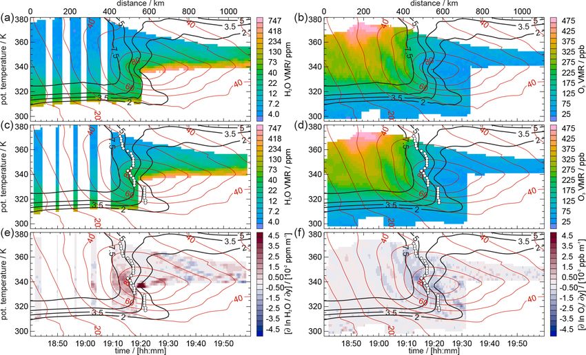
A. Schäfler et al.: Mixing at the extratropical tropopause 5221
2.3 Meteorological data
Unfortunately, no collocated profile observations of wind
and temperature are available to provide a similar resolu-
tion and coverage as the DIAL data. In order to put the
observational data in the context of the dynamical situa-
tion, we use 1-hourly meteorological reanalysis fields from
the European Centre for Medium-Range Weather Forecasts
(ECMWF) ERA5 data set (Hersbach et al., 2020) retrieved
on a 0.5◦ × 0.5◦ grid with 137 vertical levels. The reanaly-
sis fields were interpolated bilinearly in space and linearly
in time towards the observation location (Schäfler et al.,
2010). Note that the vertical separation of model levels in
the tropopause region is about 300 m (e.g., Schäfler et al.,
2020). The main parameters of interest are wind speed to
identify the jet stream, pressure and potential temperature for
the vertical context, and potential vorticity (PV). Please note
that 2 PVU are used for locating the dynamical tropopause.
Although analyses from numerical weather prediction mod-
els have significantly improved in the past, it is well known
that dynamic and thermodynamic quantities show uncertain-
ties especially in regions of strong vertical gradients, i.e., the
tropopause (e.g., Schäfler et al., 2020). However, it is deemed
sufficient to provide the large-scale dynamical context that
is relevant to interpret the observations. Additionally, error
sources resulting from temporal and spatial interpolation are
neglected.
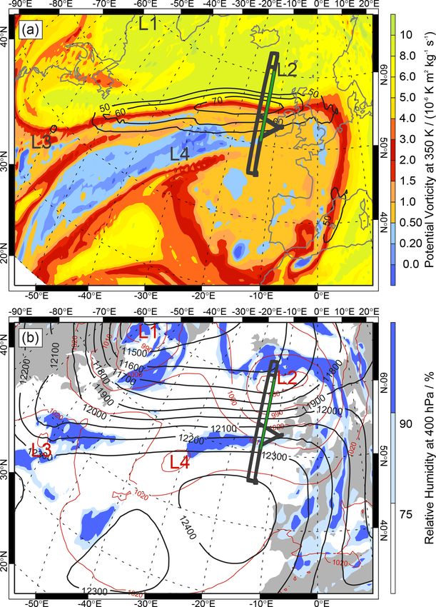
3 O3 and H2 O observations on 1 October 2017 Figure 1. (a) Potential vorticity (in colors; 10−6 K m2 kg−1 s−1 =
1 PVU) and horizontal wind speed (black contour lines; in m s−1
3.1 The synoptic setting for > 50 m s−1 ) at 350 K. (b) Relative humidity at 400 hPa (colors;
in %), geopotential height at 150 hPa (black contour lines; in m)
During the WISE campaign, a total of 17 flights were con- and surface pressure (red contour lines; in hPa) as represented in
the ECMWF operational analysis on 1 October 2017, 18:00 UTC.
ducted over the eastern North Atlantic Ocean and west-
L1–L4 mark the location of surface cyclones. Panels (a) and (b) are
ern Europe with HALO out of Shannon, Ireland, between
superimposed by the HALO flight track (12:05–21:57 UTC; thick
13 September and 21 October 2017. Collocated O3 and H2 O black line) and the subsection from 18:40 to 20:00 UTC (green line)
DIAL measurements were made in a number of meteorolog- that is discussed in this paper.
ical situations including several crossings of extratropical jet
streams and tropopause folds, multiple high-altitude observa-
tions of warm conveyor belt (WCB) outflows, i.e., strongly
ascending tropospheric air streams reaching the tropopause cal transport of tropospheric air ahead of the trough. Further
(Browning et al., 1973; Wernli and Davies, 1997), and sev- downstream, a surface cyclone was located between the UK
eral crossings of filamentary structures in occluded frontal and Iceland (L2) and another surface low (L4) is visible over
systems, i.e., typical phenomena related to breaking Rossby the central North Atlantic south of the strong jet stream. The
waves. A case study on in situ observations above a WCB 350 K PV distribution intersects with the jet stream that fol-
outflow is discussed in Kunkel et al. (2019). lows the maximum gradient in PV (Martius et al., 2010) and
Here, we focus on one particular case on 1 October 2017 separates stratospheric air (> 2 PVU) north of the wind speed
that was characterized by a straight southwesterly jet stream maximum from tropospheric air (< 2 PVU) to its south. In
over the North Atlantic Ocean (Fig. 1a) located between a this region of strong horizontal and vertical velocity gradi-
large-scale longwave trough over the western Atlantic and ents and neighboring air masses of different origin, isentropic
a ridge extending over the North Sea into southern Scan- mixing was expected to have influenced the ExTL. The syn-
dinavia (Fig. 1b). Two surface cyclones evolved in the up- optic pattern was found to be relatively persistent over the
stream trough (L1 and L3 in Fig. 1) that feature typical cy- preceding hours. Stratospheric air was transported all around
clonic cloud patterns at 400 hPa which are indicative of verti- the subtropical anticyclone keeping its high levels of PV in
https://doi.org/10.5194/acp-21-5217-2021 Atmos. Chem. Phys., 21, 5217–5234, 2021
5222                                                                A. Schäfler et al.: Mixing at the extratropical tropopause

                                                                    ing a total of 200 lidar profiles that are shown for an altitude
                                                                    range between 2.5 and 14 km. In the first 400 km, the dy-
                                                                    namical tropopause (2 PVU) is located at altitudes between
                                                                    7.5 and 8.5 km before it slopes down to about 5 km altitude.
                                                                    At about half of the flight leg, a steep ascent of the dynam-
                                                                    ical tropopause is accompanied by tropospheric air masses
                                                                    reaching altitudes up to ∼ 14 km further south. The strato-
                                                                    spheric air is characterized by increased static stability as is
                                                                    visible from the increased vertical potential temperature gra-
                                                                    dient. Westerly jet stream winds with maximum wind speeds
                                                                    up to 90 m s−1 at 9 km altitude and strong horizontal and ver-
                                                                    tical wind speed shear blow perpendicular to the flight track.
                                                                    Isentropes intersect the dynamical tropopause between 314
                                                                    and 366 K of which the lowest ones extend downward in as-
                                                                    sociation with folding of the tropopause which is typically
                                                                    initiated by ageostrophic circulation around the jet stream
                                                                    causing an intrusion of stratospheric air (Keyser and Shapiro,
                                                                    1986).
                                                                       H2 O shows the lowest VMRs (3–7 ppm) at the highest po-
Figure 2. Meteosat SEVIRI infrared satellite image (10.8 µm) for    tential temperature in the stratosphere which are typical val-
1 October 2017 at 18:00 UTC superimposed by the HALO flight         ues for autumn in the lowermost stratosphere (e.g., Zahn et
track (12:05–21:57 UTC; thick black line) and the subsection from   al., 2014). In contrast, the highest H2 O VMRs occur in the
18:40 to 20:00 UTC (orange line). Copyright 2020 EUMETSAT.          troposphere to the north and south of the jet stream ranging
                                                                    from ∼ 100 to 1000 ppm. The moist tropospheric air north of
                                                                    the jet stream is relatively well-mixed and provides typical
contrast to the tropospheric low-PV air that was advected           autumnal values for the upper troposphere of 100–300 ppm.
northeastward on the leading edge of the upstream longwave          The high-reaching tropospheric air to the south of the jet
trough filling the center of the anticyclone (Fig. 1a).             stream is more stratified. H2 O quickly decreases above a
   HALO performed a flight between 12:04 and 21:57 UTC              shallow (1–1.5 km) moist layer (100–1000 ppm) in the low-
that aimed at observing predicted strong tracer gradients           est part. The highest H2 O VMRs are indicative of recent
and mixing across the jet stream using both in situ and re-         vertical transport (e.g., in WCBs) from the moist lower tro-
mote sensing instrumentation. Multiple, almost perpendic-           posphere (Zahn et al., 2014). Furthermore, the stratification
ular crossings of the jet stream at 13 and 15◦ W were per-          and some filamentary structures with enhanced H2 O at up-
formed along a rectangular-shaped flight pattern at differ-         per levels suggest differential transport impacting the distri-
ent altitudes for in situ (FL 280, FL 410, FL 430) and              bution of the upper-tropospheric air. The lowest H2 O VMR
remote sensing measurements (FL 450, ∼ 14 km). In this              (10–40 ppm) at the highest levels and the exceptionally high
study, we concentrate on the last jet stream transect at 13◦ W      dynamical tropopause and potential temperatures are indica-
from 18:40 to 20:00 UTC (green line in Fig. 1) only, pro-           tive of transport from the subtropical or tropical upper tropo-
viding maximum data coverage beneath the aircraft at FL             sphere (UT). Missing data below the moist layer stem from
450. As this study focuses on processes in the jet stream,          midlevel clouds (see Figs. 1b and 2), while, in the first half
the northern- and the southernmost parts of the meridional          of the flight, the data gap below ∼ 5.5 km results from atten-
flight track were omitted. In those parts of the flight, either     uation of the laser signal in lower and moister air. Vertical
air mass transport in the occluded cyclone L2 or older strato-      stripes of missing H2 O data are the result of cooling issues
spheric air that was advected around the upper-level anti-          intermittently occurring at high flight altitudes with high po-
cyclone (Fig. 1a) were encountered which are not relevant           tential temperatures.
for this study. On the considered transect between 50.5 and            In addition, observed O3 values represent typical concen-
60.5◦ N, HALO crossed a zonally extended cloud band re-             trations for the season (cf. Krebsbach et al., 2006). In con-
lated to cyclone L4 (see Figs. 1b and 2) which coincides with       trast to H2 O, the highest O3 (O3 VMR of 300–500 ppb) was
the jet axis on the northern side of the clouds.                    measured in the lowermost stratosphere (LMS) with a strong
                                                                    decrease towards lower altitudes and the south. Although the
3.2    O3 and H2 O along the observed cross sections                region of the highest O3 is relatively compact, it shows large
                                                                    inhomogeneity on smaller scales with two filamentary struc-
Figure 3 shows the observed distributions of H2 O and O3            tures of increased VMR extending across isentropes towards
along the above-described ∼ 1100 km long meridionally ori-          the intrusion located below the jet stream where air is adia-
ented cross section between 18:40 and 20:00 UTC, compris-           batically transported towards the ground. In the troposphere,

Atmos. Chem. Phys., 21, 5217–5234, 2021                                               https://doi.org/10.5194/acp-21-5217-2021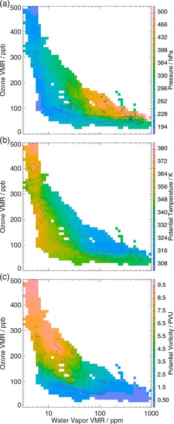
A. Schäfler et al.: Mixing at the extratropical tropopause                                                                         5223

Figure 3. DIAL observations (in colors) of (a) H2 O volume mixing ratio (VMR; in ppm = 10−6 mol mol−1 = µmol mol−1 ) and (b) O3
VMR (in ppb = 10−9 mol mol−1 = nmol mol−1 ) on 1 October 2017 (see Fig. 1 for the flight track). Panels (a) and (b) are superimposed
by horizontal wind speed (red contours; in m s−1 for wind speeds > 30 m s−1 ), potential temperature (black contours; in K) and dynamical
tropopause (2 PVU; thick black contour) interpolated from 1-hourly ECMWF ERA5 reanalyses.

O3 is comparatively low (20–100 ppb) with the lowest val-              give a first rough depiction of the tropospheric branch that
ues occurring in the mid-tropospheric moist air to the south           holds variable H2 O with VMRs covering 4 orders of mag-
of the jet stream being indicative of recent transport from the        nitude and featuring two maxima between 10 and 40 ppm
lower troposphere. The tropopause fold redistributes O3 and            and 100 and 300 ppm. The stratospheric branch is imme-
H2 O with O3 decreasing and H2 O increasing at its sides.              diately identified by H2 O observations with VMRs of less
   Note that only collocated data along the cross section are          than ∼ 7 ppm. In between both branches, collections of mix-
used in the following T–T diagnostics which covered the                ing lines form compact traces with increased numbers of
lower stratosphere north of the jet stream and a part of the up-       observations that will be called mixing regimes in the fol-
per troposphere on both sides. Therefore, it is well-suited to         lowing. The arc-shaped mixing regime that is split in two
investigate the ExTL. Note that due to the presence of clouds          traces at higher ozone concentrations connects stratospheric
no collocated observations are available in the lower part of          O3 VMRs of 250–350 ppb with tropospheric H2 O VMRs of
the tropopause fold.                                                   30–70 ppm. Interestingly, an area to the right of this arc-
                                                                       shaped mixing regime with a low number of observations
3.3   O3 and H2 O as tracer–tracer correlations                        suggests mixing between already mixed air and more humid
                                                                       (H2 O VMR of 100–200 ppm) tropospheric air. The lower
In T–T space, the collocated O3 and H2 O lidar measure-                left area in T–T space, connecting very dry tropospheric air
ments (Fig. 4a) form an L-shaped distribution with an arc-             (H2 O VMR of 8–15 ppm) and ozone-rich stratospheric air
shaped transition in between which immediately highlights              (O3 VMR > 250 ppb) is less obvious as it may be part of the
that the DIAL observations are suited to distinguish strato-           dry and ozone-poor stratospheric branch typically originat-
spheric, tropospheric and mixed air masses. In order to bet-           ing from low-latitudes (e.g., Tilmes et al., 2010) or it may be
ter characterize the partly superposed measurements, Fig. 4b           related to the mixing of dry subtropical tropospheric air with
shows the number of observations contributing to individual            ozone-rich stratospheric air. The former appears less likely
bins in the T–T diagram. O3 values of less than ∼ 100 ppb              as climatological midlatitude distributions show such pure

https://doi.org/10.5194/acp-21-5217-2021                                                 Atmos. Chem. Phys., 21, 5217–5234, 2021
5224 A. Schäfler et al.: Mixing at the extratropical tropopause
Table 1. Thresholds used for the air mass classification of tropo- features low pressures indicating that the transition occurred
spheric and stratospheric air in T–T space (see also Fig. 4). at high altitudes. High and relatively constant potential tem-
peratures suggest an isentropic mixing regime within MIX-1.
Class O3 (ppb) H2 O (ppm) The lower the pressure (the higher the potential temperature)
STRA > 280 100 across the jet stream (e.g., Zahn et al., 2014). Within MIX-2,
pressure and its variability increase towards the tropospheric
branch, while potential temperature decreases. The higher
the altitude (higher potential temperature and lower pressure)
stratospheric air masses at very low H2 O only during north- was, the lower the H2 O VMR and O3 VMR were observed
ern hemispheric winter (Hegglin et al., 2009). Additionally, in MIX-2. The area within MIX-2 that shows a separated and
H2 O is slightly increased compared to the stratospheric back- rather linear trace (Fig. 4b) features the highest potential tem-
ground with H2 O VMR of 4–7 ppm (cf. Zahn et al., 2014) perature and lowest pressure. MIX-3 occurs at low potential
leading to a somewhat reduced slope compared to the strato- temperatures and higher pressures.
spheric branch. Please note that the above-described tropo- Figure 5c shows the distribution of PV which is a tracer
spheric and stratospheric entry VMRs represent typical val- for stratospheric air comparable to O3 as it has comparable
ues with respect to climatology (Hegglin et al., 2009). Based gradients across the tropopause with high values in the stably
on these findings, Fig. 4c introduces a classification of the ob- stratified stratosphere (e.g., Shapiro, 1980). As expected, PV
served air masses solely based on their location in T–T space is highest in STRA and strongly decreases along the mixing
for this quasi-instantaneous jet stream cross section. The regimes with decreasing O3 . The mixed air masses show PV
light blue area covers the stratospheric branch (STRA) with values between 2 and 7 PVU. Furthermore, PV is found to
VMR O3 > 280 ppb and VMR H2 O < 7 ppm. The tropo- be variable within the regimes in the ExTL. Therefore, it is
spheric branch is subdivided into three classes with slightly assumed that the interrelation of the dynamical and chemical
varying O3 thresholds depending on the measurement fre- transition depends on altitude (potential temperature), a cir-
quencies in Fig. 4b. TRO-1 represents the driest tropospheric cumstance that will be discussed in more detail in Sect. 3.5.
air (VMR H2 O < 30 ppm), TRO-2 the intermediate air mass The lowest PV values are correlated with low O3 values in
(30 ppm 100 ppm) and TRO-3 the moistest the troposphere indicating more recent transport from the
air mass (VMR H2 O > 100 ppm). Table 1 summarizes the lower troposphere.
applied thresholds to detect tropospheric and stratospheric
air. The three above-discussed mixing regimes are colored in 3.4 A combined view of O3 and H2 O in T–T and
dark green (MIX-1), green (MIX-2) and light green (MIX-3) geometrical space
and connect the stratospheric branch with different parts of
the troposphere. The threshold between TRO-1 and TRO-2 A back projection of the air mass classification from T–T
was adapted to represent the tropospheric end of transitions space (Fig. 4c) into geometrical space along the cross section
within MIX-1 and MIX-2. The distribution of these air mass gives more detailed information on the shape and composi-
classes in geometrical space are further detailed in Sect. 3.4. tion of the ExTL (Fig. 6). First, it is striking that the differ-
Figure 5 shows mean and variability in pressure, potential ent air masses correspond to remarkably coherent areas along
temperature and PV for each bin in the T–T diagram. STRA the cross section. The mixed air masses in the ExTL (MIX-1,
provides low pressures and high potential temperatures that MIX-2 and MIX-3) reach about ∼ 30 K above the dynami-
decrease towards lower O3 , which corresponds to vertically cal tropopause in the northern part before they ascend with
decreasing O3 values (Fig. 3b). The increased variability in the rising tropopause further to the south. MIX-1 occurs at
pressure at lower O3 VMRs within STRA can be explained the highest altitudes in the upper part of the jet stream with
by the additional latitudinal decrease in O3 at the highest alti- its bottom being relatively well defined by the 348 K isen-
tudes (low potential temperatures). The dry tropospheric air trope. MIX-1 connects STRA with TRO-1 (isentropic tran-
mass TRO-1 also provides low pressure and high potential sition) which underlines the validity of considering MIX-1
temperature. Conversely, TRO-2 and TRO-3 possess higher as being mixed air instead of stratospheric background. The
pressure and lower potential temperature. The lowest tropo- relatively constant potential temperature along the mixing
spheric O3 corresponds to air at ∼ 8–10 km altitude on the regime (Fig. 5b) suggests the relevance of mixing processes
southern side of the jet stream. Towards higher O3 , pressure in the upper-part of the jet stream.
increases (potential temperature decreases) within TRO-2 Below, MIX-2 comprises isentropic transitions of STRA
and TRO-3 accompanied by increased variability which cor- with TRO-2 and TRO-3 above the clouds in the troposphere,
responds to tropospheric observations at different altitudes as well as cross-isentropic vertical transitions in the north-
on the northern and southern side of the jet stream. MIX-1 ern part of the flight between STRA and TRO-3. In the
Atmos. Chem. Phys., 21, 5217–5234, 2021 https://doi.org/10.5194/acp-21-5217-2021A. Schäfler et al.: Mixing at the extratropical tropopause 5225
Figure 4. Tracer–tracer (T–T) correlations of O3 and H2 O for the Figure 5. T–T correlation as in Fig. 4b but for mean (in colors)
collocated DIAL data on 1 October 2017. (a) All collocated obser- and standard deviation (gray contours) of (a) pressure, (b) potential
vations, (b) number of data points and (c) air mass classification for temperature and (c) potential vorticity.
bins in T–T space (bin sizes of 10 ppb for VMR O3 and 0.05 ppm
of log10 (VMR H2 O)).
also separates TRO-1 from TRO-2 in the tropospheric air,
which points to different source regions of humidity in the
northern part of the flight section, the bottom of the ExTL troposphere. STRA is located at the highest altitudes and in
(MIX-2) agrees with the dynamical tropopause, while the the most northern part.
thermal tropopause lies within the ExTL and approximately To further investigate the structure and strength of strato-
follows the 3.5 PVU contour. Please note that the ther- sphere to troposphere transitions within the ExTL, the con-
mal tropopause provides a typical split structure near the cept of the mixing degree metric firstly introduced by Kunz et
jet stream, while the dynamical tropopause proceeds verti- al. (2009) is advantageous. It is a measure of how much an air
cally (e.g., Randel et al., 2007). The agreement of the al- mass deviates from the background due to mixing in its previ-
most vertical dynamical tropopause and the border to the tro- ous history and is solely based on the location of the observed
pospheric air (TRO-1–TRO-3) is less uniform, and TRO-1 air mass in T–T space. Here, we adapt this concept to the li-
and TRO-2 air masses reach into areas north of the dynami- dar data, but unlike Kunz et al. (2009), the presented mixing
cal tropopause. MIX-3 occurs in the lowest observed part of factor herein is only a function of distance from the undis-
the intrusion that was observed before reaching the clouds. turbed stratospheric and tropospheric background. It does not
The geometrical location points to mixing processes between account for the distance to the intersection point of tropo-
mixed ExTL air masses and the TRO-3 air mass below in the spheric and stratospheric branches as a mixing event is not
lower part of the jet stream. Note that the 348 K isentrope considered to be stronger in the case of the tropospheric H2 O
https://doi.org/10.5194/acp-21-5217-2021 Atmos. Chem. Phys., 21, 5217–5234, 20215226 A. Schäfler et al.: Mixing at the extratropical tropopause
Figure 6. Collocated observations colored by the air mass classification in Fig. 4c. Superimposed model information as in Fig. 3 with an
additional PV contour for 3.5 PVU. Pink circles mark the thermal tropopause according to the temperature lapse rate criterion (WMO, 1957).
VMR and stratospheric O3 VMR being increased. At first, di- Figure 8 shows how observations in certain subregions
mensionless variables x and y are calculated from the VMR along the lidar cross section become apparent in T–T dis-
H2 O and VMR O3 with tributions. Profiles before 19:00 UTC (Fig. 8a) represent ver-
tical transitions in the first part of the flight that form transi-
(log (H2 O) − log (H2 OMIN )) tions from high O3 in the stratosphere along the arc-shaped
x= and
(log (H2 OMAX ) − log (H2 OMIN )) mixed region in T–T space into TRO-3 (Fig. 8b). Within the
O3 − O3,MIN
ExTL (MIX-2) the mixing lines connect comparably high
y= , stratospheric O3 (∼ 300 ppb) with high tropospheric H2 O
O3,MAX − O3,MIN (∼ 50 ppm). The tropospheric air is rather rich in O3 and
does not reach the highest levels of H2 O within TRO-3. Fig-
using the thresholds H2 OMIN = 6.5 ppm, H2 OMAX = ure 8c and d show the layer 335 to 340 K between 19:00
1000 ppm, O3,MIN = 90 ppb and O3,MAX = 500 ppb to select and 19:45 UTC, representing the above-discussed rapid tran-
the mixed air mass. The observations with lower VMRs than sition between tropospheric and ExTL air at the level of the
this range are considered to be unmixed tropospheric and jet stream maximum winds connecting TRO-3 and MIX-2.
stratospheric air. In order to range from 0 (pure stratospheric Both air masses are clearly separated in T–T space with H2 O
air) to 1 (pure tropospheric air), the mixing factor f is VMRs jumping from ∼ 50 ppm at the tropospheric end of
calculated for x > y as f = 1 − (0.5 · (y/x)) and for x < y MIX-2 to ∼ 500 ppm in TRO-3 (Fig. 8d) over a very short
as f = 0.5 · (x/y). spatial distance (Fig. 8c) indicating minor mixing between
Figure 7a shows the observations color-coded by the mix- both air masses. The more stratospheric part of MIX-2 fol-
ing factor. Please note that the selected ExTL air masses lows the arc-shaped distribution, while the tropospheric part
slightly differ from Fig. 4 due to the application of con- that is facing the jet stream is slightly detached (Fig. 8d),
stant minimum thresholds. The back projection of the mix- which potentially indicates different mixing processes within
ing factor in Fig. 7b picks up the major transition regions this particular layer. Interestingly, the layer directly above
in MIX-1, MIX-2 and MIX-3. At the highest levels (above (340–347 K; Fig. 8e) that represents the transition of MIX-2
350 K), i.e., directly above the jet stream maximum winds, air with medium moist air in TRO-2 is relatively abrupt
the isentropic transition is rather uniform. In the layer be- but the discontinuity occurs within the ExTL (Fig. 8f), i.e.,
neath (340–350 K), rapid transitions result in a lack of ob- between the linear-shaped stratospheric part and the tropo-
servations with intermediate chemical characteristics. Below spheric end, suggesting some in-mixing of TRO-2 air into
potential temperatures of 340 K, the transition is again more this layer. The location of these abrupt transitions in the two
uniform. Within the tropopause fold air masses with interme- layers between 337 and 347 K occurs at the same spatial loca-
diate chemical composition are transported towards the lower tion (cf. Fig. 7b). Both layers do not reach far into the LMS.
troposphere. The above-described stratospheric filaments of The situation appears different in the upper part between
high O3 correspond to decreased mixing factors indicating 349 and 358 K where the mixing factor diagnostic shows
the stratospheric character of the observed air compared to more uniform transitions (Fig. 7b). The layer that connects
the surroundings. Figures 6 and 7b suggest that both verti- LMS air in STRA with low H2 O VMRs in TRO-1 (Fig. 8g)
cal (MIX-2) and isentropic transitions (MIX-1 and MIX-2) shows more gradual transitions across MIX-1 in T–T space
formed the mixing lines.
Atmos. Chem. Phys., 21, 5217–5234, 2021 https://doi.org/10.5194/acp-21-5217-2021A. Schäfler et al.: Mixing at the extratropical tropopause 5227
Figure 7. Mixing factor diagnostic for all collocated measurements in (a) T–T space using lower limits for H2 O VMR of 6.5 ppm and for O3
VMR of 90 ppb for selecting mixed air masses (for details see text) and (b) projected back to geometrical space.
(Fig. 8h). Please note that the minimum number of observa- PV distributions on isentropes that required smoothing using
tions within MIX-1 (O3 VMR 200–250 ppm) is a result of a moving average. For this reason, PV contours in Fig. 9c
the data gap between 19:06 and 19:08 UTC. Figure 8i and j and d appear slightly smoothed. Consistent with Kunz et
show the vertical transitions at the bottom of the tropopause al. (2011a), the PV-gradient tropopause is shifted to higher
fold that unlike the vertical transitions in Fig. 8a and b show PV values with increasing potential temperature. It approxi-
a mixing of ExTL air (MIX-2) and tropospheric air (TRO-3) mately follows the curvy shape of individual PV isolines.
below. To calculate isentropic trace gas gradients from the obser-
vational data, O3 and H2 O are also smoothed (Fig. 9c and d)
3.5 Chemical and dynamical discontinuities at the to account for instrument-generated noise causing strong lo-
tropopause cal gradients. Note that smoothing of the H2 O data increased
the data gaps before 19:10 UTC. Trace gas gradients were
Section 3.3 and 3.4 confirmed earlier findings that the 2 PVU then calculated for the natural logarithm of the trace gas con-
dynamical tropopause marks the bottom of the ExTL north centration as suggested by Kunz et al. (2011b) with the pur-
of the jet stream. However, where the dynamical tropopause pose of scaling down increased gradients in the source re-
is almost vertical, its location relative to the ExTL bound- gions at higher concentrations of the trace gas (stratosphere
ary is found to be variable (Fig. 6). Additionally, the mixing for O3 and troposphere for H2 O). This shifts the focus to-
factor metric shown (Fig. 7b) indicates differing strengths in wards the gradients across the tropopause. Strongest isen-
the ExTL transition at different layers within the jet stream. tropic gradients of H2 O are found at the level of maximum
Figure 9a and b show regridded versions of the O3 and H2 O winds within the ExTL (MIX-2), while above H2 O gradients
cross sections using potential temperature as the vertical co- are weaker where tropospheric H2 O VMR (TRO-1) is lower
ordinate. As in Fig. 3a and b, all available O3 and H2 O ob- and mixing within MIX-2 is more uniform (Fig. 9e and f).
servations are used for maximum data coverage to deter- Please note that the highest local gradient at ∼ 19:20 UTC
mine isentropic gradients. Obviously, the stratospheric air is related to a very high H2 O VMR at the edge of the
with its strong vertical gradients in potential temperature gets cloud layer. O3 with higher coverage in the lower part of
stretched, while the tropospheric part shrinks in isentropic the tropopause fold also indicates maximum gradients at the
coordinates. level of maximum winds. Additionally, an increased O3 gra-
The jet stream maximum is located at ∼ 340 K with the dient occurs at the bottom of the fold as compared to H2 O.
2 PVU isoline crossing it. Higher PV isolines appear north O3 gradients are smaller above 350 K. Some increased pos-
of the jet. In addition to arbitrarily selected PV thresholds itive and negative gradients are found in the stratosphere re-
for the dynamical tropopause (Hoerling et al., 1991), Kunz lated to the O3 filament. The PV-gradient tropopause better
et al. (2011a) introduced a dynamical tropopause which is represents the regions of the highest isentropic trace gas gra-
defined as the maximum isentropic PV gradient which is dients than the 2 PVU isoline, especially in the case of the
maximized near jet streams (Martius et al., 2010). The PV- O3 gradients. It follows the center of maximum O3 gradi-
gradient tropopause is constrained by the wind speed to cor- ents at the level of highest wind speeds and above. Max-
rectly identify high wind speed situations near polar and sub- imum H2 O gradients are located north of the PV-gradient
tropical jet streams. Figure 9c and d depict the PV-gradient tropopause at even higher PV values at the jet stream level
tropopause along the isentropes in the latitudinal cross sec- where pronounced gradients are visible. Kunz et al. (2011b)
tion. Note that the quasi-linear interpolation between grid- argue that the better agreement of the PV-gradient tropopause
ded model data along the 15◦ W meridian resulted in edged
https://doi.org/10.5194/acp-21-5217-2021 Atmos. Chem. Phys., 21, 5217–5234, 20215228 A. Schäfler et al.: Mixing at the extratropical tropopause
Figure 8. Data subsets of the collocated lidar data. (a, b) Before 19:00 UTC with (a) showing the data as classified in Fig. 6 and in (b) as
black dots superimposed on the classification of all data shown in Fig. 4c. (c, d) As (a) and (b) but for data in the time period from 19:00 to
19:45 UTC in the layer 335–340 K. (e, f) For 19:00 to 19:45 UTC and 340–347 K. (g, h) For 19:00 to 19:45 UTC and 349–358 K. (i, j) For
19:15 to 19:21 UTC and 311–324 K.
with the stratospheric tracer originates from their common 4 Summary and discussion
stratospheric concept, in the sense that the chemical tracer O3
and the dynamical tracer PV are higher in the stratosphere. In
In this study we analyze the mixing of air masses at the extra-
contrast H2 O exhibits stronger tropospheric gradients which
tropical tropopause that shapes the structure and the chemical
are mostly related to transport processes into the UT.
composition of the ExTL with the first-ever set of collocated
O3 and H2 O lidar observations obtained during the WISE
field campaign over the North Atlantic Ocean in autumn
Atmos. Chem. Phys., 21, 5217–5234, 2021 https://doi.org/10.5194/acp-21-5217-2021A. Schäfler et al.: Mixing at the extratropical tropopause 5229
Figure 9. Regridded DIAL observations of (a) H2 O and (b) O3 (as shown in Fig. 3) using potential temperature as the vertical coordinate
(same profile locations and for potential temperature bins of 2 K). (c, d) As (a) and (b) but using a moving average filter along isentropic
levels (using 7 observations for H2 O and O3 and 13 model values for PV and wind speed). Panels (e) and (f) show isentropic gradients of the
natural logarithm of VMR H2 O and VMR O3 based on the isentropically smoothed data. All panels are superimposed by PV contours (2,
3.5, 5 and 7.5 PVU; thick black contours) and wind speed (in m s−1 for > 30 m s−1 ). White dots in (c)–(f) mark the PV-gradient tropopause
based on maximum gradients of isentropic PV and winds following Kunz et al. (2011a) (for details see text).
2017. We demonstrate the potential of quasi-instantaneous 2004). The lidar observations allow the ExTL to be deter-
O3 and H2 O cross-section observations in a dynamically mined for an individual but representative dynamic situation.
rather simple synoptic situation with a perpendicular cross- The 2D depiction represents the first and almost complete
ing of a straight southwesterly jet stream. The presented observation-based illustration of the ExTL and confirmation
flight on 1 October 2017 captured a low tropopause on the of the conceptual model in Gettelman et al. (2011) that shows
northern cyclonic shear side of the jet stream and a high the ExTL following the tropopause. So far, this concept was
tropopause with high-reaching tropospheric air to its south. based on studies using a limited number of in situ flight legs
In between, a tropopause fold extended downward along at different altitudes or model simulations (e.g., Pan et al.,
tilted isentropes into the lower tropospheric frontal zone be- 2007; Vogel et al., 2011; Konopka and Pan, 2012).
fore the tropopause strongly ascended accompanied by an We further demonstrate that probability densities in T–T
upper-level frontal zone above the jet stream. This flight pro- space enable us to identify certain clusters of mixing lines
vides exceptionally good data coverage due to low cloud cov- (i.e., mixing regimes) and to classify subsets of mixed and
erage beneath the aircraft and a high flight altitude. tropospheric air. These classes show a remarkably coherent
The collocated and range-resolved O3 and H2 O lidar pro- structure in geometrical space. In the upper part of the jet
file data along the cross section feature typical values for the stream, ozone-rich stratospheric air and dry tropospheric air
season, latitude and altitude range when compared to cli- are connected via a distinct mixing regime. Below, a sepa-
matological values. We show that the precision of the data rated mixing regime links stratospheric air with moister tro-
at a horizontal resolution of 5.6 km is suitable to identify pospheric air. Although these mixed air masses are clearly
the ExTL and to depict its shape and composition in un- separated in T–T space, we illustrate that they are stacked
precedented detail by applying established T–T diagnostics. directly on top of each other in geometrical space. As the
Through a back projection of T–T-derived information to separation in the tropospheric and the mixed air occurs at the
geometrical space, i.e., along the cross section, physically same potential temperature (∼ 348 K), we hypothesize that
meaningful thresholds were selected for the air mass clas- different transport pathways in this particular dynamic sit-
sification that so far was barely possible (e.g., Pan et al., uation brought air with differing H2 O VMRs to the upper-
https://doi.org/10.5194/acp-21-5217-2021 Atmos. Chem. Phys., 21, 5217–5234, 2021You can also read