A new method to detect and classify polar stratospheric nitric acid trihydrate clouds derived from radiative transfer simulations and its first ...
←
→
Page content transcription
If your browser does not render page correctly, please read the page content below
Atmos. Meas. Tech., 14, 1893–1915, 2021
https://doi.org/10.5194/amt-14-1893-2021
This work is distributed under
the Creative Commons Attribution 4.0 License.

A new method to detect and classify polar stratospheric nitric acid
trihydrate clouds derived from radiative transfer simulations and its
first application to airborne infrared limb emission observations
Christoph Kalicinsky1 , Sabine Griessbach2 , and Reinhold Spang3
1 Institute
          for Atmospheric and Environmental Research, University of Wuppertal, Wuppertal, Germany
2 Forschungszentrum Jülich, Jülich Supercomputing Centre (JSC), Jülich, Germany
3 Forschungszentrum Jülich, Institut für Energie und Klimaforschung, Stratosphäre (IEK-7), Jülich, Germany

Correspondence: Christoph Kalicinsky (kalicins@uni-wuppertal.de)

Received: 15 April 2020 – Discussion started: 27 July 2020
Revised: 9 December 2020 – Accepted: 18 December 2020 – Published: 9 March 2021

Abstract. Polar stratospheric clouds (PSCs) play an impor-       ance of the spectral feature, we defined different colour in-
tant role in the spatial and temporal evolution of trace gases   dices to detect PSCs containing NAT particles and to sub-
inside the polar vortex due to different processes, such as      group them into three size regimes under the assumption
chlorine activation and NOy redistribution. As there are still   of spherical particles: small NAT (≤ 1.0 µm), medium NAT
uncertainties in the representation of PSCs in model simula-     (1.5–4.0 µm), and large NAT (≥ 3.5 µm). Furthermore, we
tions, detailed observations of PSCs and information on their    developed a method to detect the bottom altitude of a cloud
type – nitric acid trihydrate (NAT), supercooled ternary solu-   by using the cloud index (CI), a colour ratio indicating the
tion (STS), and ice – are desirable.                             optical thickness, and the vertical gradient of the CI. Finally,
   The measurements inside PSCs made by the CRISTA-NF            we applied the methods to observations of the CRISTA-NF
(CRyogenic Infrared Spectrometers and Telescope for the          instrument during one local flight of the RECONCILE air-
Atmosphere – New Frontiers) airborne infrared limb sounder       craft campaign and found STS and medium-sized NAT.
during the RECONCILE (Reconciliation of essential process
parameters for an enhanced predictability of Arctic strato-
spheric ozone loss and its climate interactions) aircraft cam-
paign showed a spectral peak at about 816 cm−1 . This peak
is shifted compared with the known peak at about 820 cm−1 ,      1   Introduction
which is recognised as being caused by the emission of ra-
diation by small NAT particles. To investigate the reason for    Polar stratospheric clouds (PSCs) form inside the cold po-
this spectral difference, we performed a large set of radia-     lar vortices in both hemispheres in winter. They have a ma-
tive transfer simulations of infrared limb emission spectra      jor influence on the ozone chemistry and, thus, ozone deple-
in the presence of various PSCs (NAT, STS, ice, and mix-         tion in the stratosphere (Solomon, 1999). PSCs are classi-
tures) for the airborne viewing geometry of CRISTA-NF.           fied into three different types: supercooled ternary solution
NAT particles can cause different spectral features in the       (STS) droplets, nitric acid trihydrate (NAT), and ice parti-
810–820 cm−1 region. The simulation results show that the        cles (e.g. Lowe and MacKenzie, 2008). The formation and
appearance of the feature changes with an increasing median      existence of these different types is largely temperature de-
radius of the NAT particle size distribution, from a peak at     pendent. Solid ice particles can only exist below the frost
820 cm−1 to a shifted peak and, finally, to a step-like fea-     point Tfrost ≈ 188 K, whereas NAT particles are thermody-
ture in the spectrum, caused by the increasing contribution      namically stable at temperatures below TNAT ≈ 195 K. The
of scattering to the total extinction. Based on the appear-      liquid STS droplets form from binary H2 SO4 –H2 O droplets
                                                                 at temperatures below the dew point of HNO3 Tdew ≈ 192 K

Published by Copernicus Publications on behalf of the European Geosciences Union.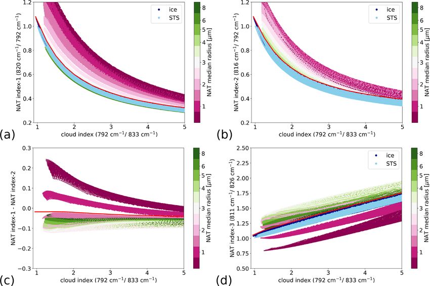
1894                                                 C. Kalicinsky et al.: Radiative transfer simulations of infrared spectra

by the uptake of HNO3 (see e.g. Peter and Grooß, 2012, and        these above-mentioned measurement techniques, an infrared
references therein).                                              limb emission sounder builds a good basis for PSC studies
   PSCs directly and indirectly influence the spatial distri-     (e.g. Spang and Remedios, 2003; Höpfner et al., 2006).
bution of trace gases relevant for ozone depletion in differ-        In addition to the derivation of volume mixing ratios of
ent ways. Due to heterogenous reactions on the cold parti-        several trace gases, infrared limb emission sounders such
cle surfaces, chlorine is activated from its reservoir species,   as CRISTA (CRyogenic Infrared Spectrometers and Tele-
mainly HCl and ClONO2 , and the chlorine radicals catalyt-        scopes for the Atmosphere; Offermann et al., 1999; Gross-
ically destroy ozone (e.g. Solomon, 1999). NAT particles          mann et al., 2002), CRISTA-NF (CRyogenic Infrared Spec-
can grow to larger sizes, which then leads to a sedimenta-        trometers and Telescope for the Atmosphere – New Fron-
tion of the particles and, thus, to a permanent removal of        tiers; Kullmann et al., 2004), and MIPAS-Envisat (Michelson
HNO3 from the stratosphere (denitrification) (e.g. Fahey et       Interferometer for Passive Atmospheric Sounding – Envisat;
al., 2001; Molleker et al., 2014). This denitrification slows     Fischer et al., 2008) are well-suited to detect clouds of dif-
down the deactivation of chlorine and, therefore, enhances        ferent composition. Spang et al. (2001) established a simple
the ozone loss (e.g. Waibel et al., 1999; Peter and Grooß,        and effective cloud detection method based on the radiance
2012).                                                            ratio of two specific spectral regions. The first one is domi-
   Because of these different processes and due to the fact       nated by CO2 molecular line emissions (around 792 cm−1 ),
that many models rely on rather simple parameterisations,         and the second one is dominated by the broader continuum-
the simulation of PSCs and related processes is incom-            like aerosol emissions (around 833 cm−1 ). This detection
plete and is also partly accompanied by larger uncertain-         method was then successfully used in various studies and
ties. Specifically, chemistry climate models (CCMs) that are      for different satellite and airborne instruments (e.g. Spang
used to assess polar stratospheric ozone loss (e.g Eyring et      and Remedios, 2003; Spang et al., 2002, 2005, 2008, 2015;
al., 2013) often employ rather simple schemes to represent        Höpfner et al., 2006; Kalicinsky et al., 2013). Furthermore,
PSCs in the model simulations. Such simplifications may           the infrared spectra exhibit different spectral features or ra-
lead to a heterogeneous chemistry dominated by NAT, but           diance behaviours in the presence of different types of polar
it is known that heterogeneous chemistry on STS and cold          stratospheric clouds. Spang and Remedios (2003) presented
binary aerosol particles probably dominates the chlorine ac-      a sharp peak-like feature at around 820 cm−1 observed by
tivation (e.g Solomon, 1999; Drdla and Müller, 2012; Kirner       the CRISTA instrument in the Antarctic winter for the first
at al., 2015). Additionally, no comprehensive microphysical       time. They attributed this feature to HNO3 -containing par-
models are typically used to describe the evolution of PSCs       ticles. Höpfner et al. (2006) showed that the feature can be
over the winter. Mesoscale temperature variations that are        best reproduced in simulations by using refractive index data
known to play an important role in the formation of PSCs          for β-NAT particles (assuming relatively high number den-
(Carslaw et al., 1998; Dörnbrack et al., 2002; Engel et al.,      sities). The authors showed that the colour ratio method de-
2013; Hoffmann et al., 2017) are also missing in current          rived by Spang and Remedios (2003) that exploits the peak-
state-of-the-art CCMs (Orr et al., 2015).                         like feature for detection is able to identify PSCs containing
   Assumptions regarding the occurrence of different PSC          small NAT particles (radii < 3 µm). By means of a large set
types typically only have a limited impact on many aspects        of radiative transfer simulations, Spang et al. (2012, 2016)
of ozone loss, as, for example, liquid PSC particles are suf-     developed a detection and discrimination method for PSCs.
ficient to simulate nearly all ozone loss (Wohltmann et al.,      Besides the feature at 820 cm−1 , the method also uses further
2013; Kirner at al., 2015; Solomon et al., 2015). However,        spectral behaviours such as a radiance decrease from around
there are also situations where the PSC type is crucial. For      830 cm−1 towards larger wavenumbers (around 950 cm−1 )
example, the specific PSC type present at the top of the          that occurs in the case of ice to distinguish different PSC
ozone loss region is important (Kirner at al., 2015), and type    types. Spang et al. (2018) finally presented a climatology of
also plays an important role during the initial activation in     the PSC composition for the whole MIPAS-Envisat observa-
PSCs covering only a small part of the vortex (Wegner et al.,     tion time period (2002–2012) based on this method.
2012). Furthermore, the heterogenous reaction rates on PSCs          During the RECONCILE campaign (Reconciliation of es-
strongly depend on temperature as well as on the PSC type         sential process parameters for an enhanced predictability of
(e.g. Drdla and Müller, 2012; Wegner et al., 2012). Here, es-     Arctic stratospheric ozone loss and its climate interactions;
pecially for NAT, the reaction rates show rather large uncer-     von Hobe et al., 2013) a slightly different type of spectral fea-
tainties (Carslaw et al., 1997; Wegner et al., 2012), which       ture was observed by the CRISTA-NF infrared limb emission
highlights the importance of observing the PSC type.              sounder in the presence of PSCs. The campaign took place in
   In summary, information on the composition of PSCs is          Kiruna, Sweden, from January to March 2010, and the high-
very important, but measurements are limited. Typical PSC         flying M55-Geophysica research aircraft carried out a num-
measurement techniques are in situ particle measurements          ber of flights with a huge set of different instruments in order
and lidar observations (e.g. Molleker et al., 2014; Achtert       to study the polar vortex and related scientific topics, such
and Tesche, 2014; Pitts et al., 2018). However, in addition to    as PSCs, ozone chemistry, and mixing processes. CRISTA-

Atmos. Meas. Tech., 14, 1893–1915, 2021                                            https://doi.org/10.5194/amt-14-1893-2021
C. Kalicinsky et al.: Radiative transfer simulations of infrared spectra                                                     1895

NF was one of the instruments operated and is able to de-          2     Methods and set-up
tect clouds and distinguish different types of PSCs. During
the first five flights of the campaign (17–25 January 2010),       The radiative transfer simulations were performed using the
CRISTA-NF detected PSCs around the aircraft. Because of            viewing geometry and spectral properties of the CRISTA-
the viewing geometry of an infrared limb sounder, where the        NF airborne infrared limb sounder. The background atmo-
horizontal distance of a tangent point to the aircraft increases   sphere used for the simulations is a polar winter atmosphere
with decreasing sampling altitude, CRISTA-NF typically ob-         with conditions suitable for the formation of polar strato-
serves air masses in a wider range around the aircraft. The in-    spheric clouds. The simulations themselves were performed
frared spectra measured inside the clouds show a noticeable        using the Juelich Rapid Spectral Simulation Code (JURAS-
spectral feature at about 816 cm−1 . This feature is slightly      SIC). This section describes the CRISTA-NF instrument, the
shifted towards smaller wavenumbers compared with the              JURASSIC radiative transfer code, the set-up used for the
typical spectral feature at 820 cm−1 , which is caused by very     simulations, and the different cloud scenarios that were in-
small NAT particles. Another appearance of the spectral fea-       vestigated.
ture caused by NAT particles, a step-like or shoulder-like be-
haviour of the radiance in the 810–820 cm−1 spectral region,       2.1    CRISTA-NF instrument
was observed by the MIPAS-B balloon-borne instrument in
January 2001 (Höpfner et al., 2002) and the MIPAS-STR air-         The airborne CRISTA-NF instrument is a successor of the
borne instrument during the ESSENCE campaign in Decem-             CRISTA satellite instrument. CRISTA-NF measures the ther-
ber 2011 (Woiwode et al., 2016). Woiwode et al. (2016) anal-       mal emissions of the atmosphere in the mid-infrared region
ysed different particle modes with radii between 1 and 6 µm        from 4 to 15 µm in an altitude range from flight altitude (up
and suggested that highly aspherical medium to large-sized         to 20 km) down to approximately 5 km. A detailed descrip-
(median radius 4.8 µm) NAT particles caused the change in          tion of the design of the cryostat and the optical system is
the NAT signature to the step-like appearance. Woiwode et al.      given by Kullmann et al. (2004). The calibration procedure
(2016) concluded that the particle shape and the scattered ra-     and some improvements for the RECONCILE campaign are
diation from below can influence the feature. However, the         described by Schroeder et al. (2009) and Ungermann et al.
appearance of the spectral feature seems to depend on the          (2012) respectively.
particle size distributions of the NAT particles, especially on       CRISTA-NF uses a Herschel telescope and a tiltable mir-
the median radius. This motivated the following study of the       ror to scan the atmosphere from flight altitude down to ap-
relationship between the appearance of the feature (typical,       proximately 5 km. The incoming radiance is then spectrally
shifted, and step-like) and the corresponding particle size dis-   dispersed by two Ebert–Fastie grating spectrometers (e.g.
tribution, aiming at an improved detection method for PSCs         Fastie, 1991). These two spectrometers have different re-
                                                                                                              λ
containing NAT particles. In particular, the possibility to de-    spective spectral resolving powers of 1λ      ≈ 1000 and 500;
tect larger NAT particles is important, because they play a        therefore, they are denoted as a high-resolution spectrometer
major role in the denitrification of the stratosphere (Fahey et    (HRS) and a low-resolution spectrometer (LRS) respectively.
al., 2001; Molleker et al., 2014) and, thus, in ozone chemistry    In this study, we focus on the spectral range that is covered
as a whole (e.g. Waibel et al., 1999; Peter and Grooß, 2012).      by the LRS 5 (850–965 cm−1 ) and LRS 6 (775–865 cm−1 )
New insights and an improvement in the detection method            channels. The vertical sampling of the LRS during one al-
are also interesting for measurements of other infrared limb       titude scan is typically between 100 and 200 m with finer
emission sounders such as MIPAS-Envisat, where data for            sampling at higher altitudes and wider sampling at lower al-
a long observation period (about 10 years) and both hemi-          titudes due to mounting and instrument conditions. The field
spheres are available. For this purpose, a large variety of dif-   of view (FOV) is very small at 3 arcmin (about 300 m at 10
ferent PSCs with respect to the composition, spatial dimen-        km tangent height; Spang et al., 2008). The horizontal sam-
sions, and particle size distributions of the PSC particles were   pling along the flight track is about 12.5 to 15 km depending
simulated and analysed.                                            on the speed of the aircraft. The radiance is finally measured
   The paper is structured as follows: in Sect. 2, the CRISTA-     using liquid helium cooled semiconductor detectors (Si : Ga)
NF instrument and the radiative transfer code are described,       that are operated at a temperature of 13 K. These low tem-
and the set-up used for the simulations is explained; the re-      peratures enable fast measurements of one spectrum in about
sults of the simulations are presented and analysed in Sect. 3;    1 s.
the derived methods are applied to the CRISTA-NF measure-
ments in Sect. 4; and, finally, the main results are discussed     2.2    The JURASSIC radiative transfer simulation code
in Sect. 5 and summarised in Sect. 6.
                                                                   For the simulations of the CRISTA-NF infrared spectra in the
                                                                   presence of PSCs, we used the Juelich Rapid Spectral Simu-
                                                                   lation Code (JURASSIC) (Hoffmann, 2006). It is a fast radia-
                                                                   tive transfer model for the mid-infrared spectral region. It has

https://doi.org/10.5194/amt-14-1893-2021                                             Atmos. Meas. Tech., 14, 1893–1915, 2021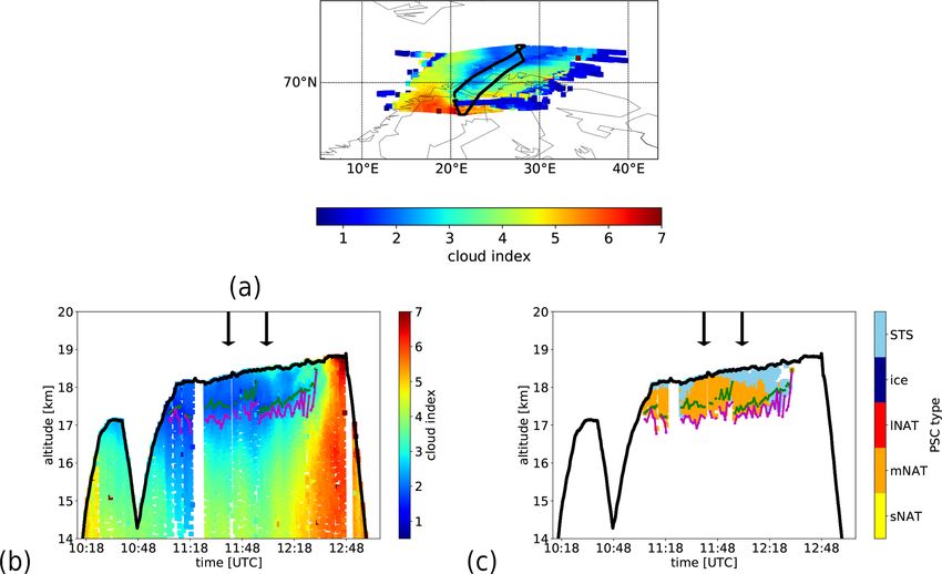
1896                                                    C. Kalicinsky et al.: Radiative transfer simulations of infrared spectra

been used in numerous studies analysing infrared limb and             Table 1. CRISTA-NF instrument properties used in the simulations.
nadir measurements, including MIPAS-Envisat (Hoffmann
et al., 2005, 2008), CRISTA-NF (Hoffmann et al., 2009;                  Property                       Value
Weigel et al., 2009), and the AIRS nadir sounder (Hoff-                 Vertical sampling              100 m
mann and Alexander, 2009), as well as to simulate 2-D trace             Spectral sampling              0.42 cm−1 for 785–840 cm−1
gas and temperature retrievals for a proposed new infrared                                             0.59 cm−1 for 940–965 cm−1
limb instrument named PREMIER IRLS (PRocess Exploita-                                             λ
                                                                        Spectral resolving power 1λ    536 at 12.5 µm
tion through Measurements of Infrared and millimetre-wave               Observer altitude              18.4 km
Emitted Radiation – InfraRed Limb Sounder; Preusse et al.,              Altitude range                 10 km – observer altitude
2009; Hoffmann and Riese, 2010). For fast radiative trans-
fer calculations, JURASSIC applies a spectral averaging ap-
proach by using the emissivity growth approximation (EGA)             sponds to an average of 0.42 cm−1 for the 785–840 cm−1
(Gordley and Russel III, 1981; Marshall et al., 1994) and pre-        wavelength range and 0.59 cm−1 for the 940–965 cm−1 re-
calculated lookup tables. The lookup tables were calculated           gion. These values have been considered in the calculation
by the line-by-line model reference forward model (RFM;               of the lookup tables for JURASSIC. We used an observer
Dudhia, 2017) and take the spectral resolution of the instru-         altitude of 18.4 km, which is the maximum average flight al-
ment to be investigated into account.                                 titude during the RECONCILE flights of interest. However,
   JURASSIC has been compared to the RFM and KOPRA                    the average altitudes of all flights only differ by a few hun-
(Karlsruhe Optimized and Precise Radiative transfer Algo-             dred metres (18.1 to 18.4 km). The observations were sim-
rithm) line-by-line models for selected spectral windows and          ulated in the tangent altitude range from observer altitude
shows good agreement (Griessbach et al., 2013). JURAS-                down to 10 km. The vertical sampling used for the simula-
SIC was extended with a scattering module that allows for             tions was 100 m. Table 1 summarises these properties.
radiative transfer simulations, including single scattering on
aerosol and cloud particles (Griessbach et al., 2013). The op-        2.3.2   Atmospheric set-up
tical properties of the particles (extinction coefficient, scatter-
ing coefficient, and phase function) required for the radiative       For the background atmosphere we used polar winter condi-
transfer simulations with scattering can either be calculated         tions to get representative simulations. Most information was
with an internal Mie code assuming spherical particles or can         taken from the MIPAS reference polar winter climatology by
be taken from databases for non-spherical particles. The scat-        Remedios et al. (2007). We updated some constituents, and
tering module has been used successfully in different studies         we focused on the winter 2009–2010 here, especially on Jan-
(Griessbach et al., 2014, 2016, 2020).                                uary 2010. There are two reasons for this choice: (1) a large
                                                                      variety of PSCs were observed in the Arctic in this winter;
2.3     Simulation set-up                                             and (2) the CRISTA-NF observations of PSCs during REC-
                                                                      ONCILE took place in January 2010. The updates are sum-
The simulation set-up can be divided into three parts: the            marised in the following.
instrument part, the atmosphere part, and the cloud scenar-              Two very important parameters of the atmosphere for the
ios. The instrument part includes the viewing geometry and            simulation of infrared spectra are temperature and CO2 vol-
the spectral properties of the CRISTA-NF airborne infrared            ume mixing ratios (VMRs). In order to have a temperature
limb emission sounder. In the atmosphere part we describe             profile that is representative for a situation where many dif-
the background atmosphere that is used for the simulations.           ferent PSCs can occur, we focused on the PSC observation
All different types of polar stratospheric clouds with respect        period during the RECONCILE aircraft campaign (17 to
to the position and thickness of the cloud as well as the com-        25 January 2010). The temperature profile was derived us-
position (NAT, STS, and ice) are summarised in the cloud              ing ERA-Interim reanalysis data (Dee et al., 2011). An av-
scenario section.                                                     erage profile in the region of the CRISTA-NF observations
                                                                      north of Kiruna (67–78◦ N, 10–35◦ E) was used for the back-
2.3.1    Instrument properties                                        ground atmosphere. Additionally, we used the correspond-
                                                                      ing pressure profile from ERA-Interim reanalysis data. The
The two important spectral regions that are necessary to anal-        CO2 VMR was derived from the reconstructed CO2 prod-
yse infrared spectra with respect to polar stratospheric clouds       uct by Diallo et al. (2017) for January 2010. The profile is
are 785–840 cm−1 , because of the cloud index (CI) and the            a zonal average in the latitude region of interest. The pro-
NAT signature, and the 940–965 cm−1 region, because of an             files were extended to larger altitudes following the slope
ice signature. The spectral resolving power used in the sim-          of the climatology. As PAN (peroxyacetyl nitrate) is not in-
             λ
ulations is 1λ  = 536 at a reference wavelength of 12.5 µm            cluded in the climatology, we took a mean profile derived
         −1
(800 cm ) (see Weigel, 2009). The spectral sampling of the            from CRISTA-NF observations (see Ungermann et al., 2012,
CRISTA-NF measurements is about 0.0065 µm and corre-                  for the retrieval description) in the region around Kiruna be-

Atmos. Meas. Tech., 14, 1893–1915, 2021                                                https://doi.org/10.5194/amt-14-1893-2021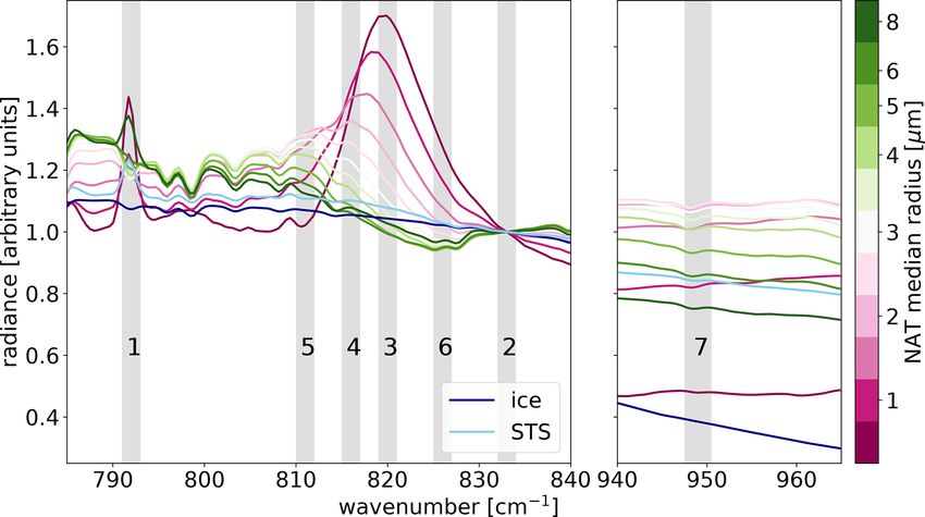
C. Kalicinsky et al.: Radiative transfer simulations of infrared spectra                                                                1897

tween the end of January and the beginning of March. Un-           Table 2. Set-up of the background atmosphere for the simulations.
fortunately, there are no retrieval results for PAN available
during the PSC flights. However, the derived profile is in          Constituent   Source                                      Spectral region
a good agreement with published MIPAS-Envisat observa-              Temperature   ERA-Interim (Dee et al., 2011)              Both
tions for October to December 2003 in the corresponding             Pressure      ERA-Interim (Dee et al., 2011)              Both
latitudinal region (Glatthor et al., 2007) and also with the
                                                                    CO2           Diallo et al. (2017)                        Both
average profile in 2007–2008 in the latitudinal band from 60
to 90◦ (Pope et al., 2016). For CFC-11, CFC-113, HCFC-              HNO3          Climatology                                 Both
22, SF6 , and COF2 , we updated the climatological profiles         O3            Climatology                                 Both
to 2010 values using information on tropospheric values             ClONO2        Climatology                                 785–840 cm−1
(Bullister, 2011) as well as satellite observations from the At-
                                                                    H2 O          Climatology                                 Both
mospheric Chemistry Experiment Fourier Transform Spec-
trometer (ACE-FTS) (Boone et al., 2013) and in situ obser-          HNO4          Climatology                                 785–840 cm−1
vations carried out by the High Altitude Gas Analyzer (HA-          CCl4          Climatology                                 785–840 cm−1
GAR) instrument (Riediger et al., 2000; Werner et al., 2010)        ClO           Climatology                                 785–840 cm−1
onboard the M55-Geophysica during RECONCILE.
                                                                    NO2           Climatology                                 785–840 cm−1
   In order to save computation time, we restricted the num-
ber of trace gases to a minimum by just using those gases           CFC-11        Climatology with update                     Both
                                                                                  (using HAGAR; Riediger et al., 2000;
that have a noticeable contribution to the total radiance in                      Werner et al., 2010; and Bullister, 2011)
the two analysed spectral regions. The trace gases have been
                                                                    HCFC-22       Climatology with update                     785–840 cm−1
selected separately for the two spectral regions. For the
                                                                                  (using ACE-FTS; Boone et al., 2013)
785–840 cm−1 region, we used 13 trace gases: CO2 , HNO3 ,
ClONO2 , O3 , H2 O, HNO4 , CCl4 , CFC-11, HCFC-22, CFC-             CFC-113       Climatology with update                     785–840 cm−1
                                                                                  (using Bullister, 2011)
113, PAN, ClO, and NO2 . The simulations in the 940–
965 cm−1 region included nine trace gases: CO2 , HNO3 , O3 ,        PAN           CRISTA-NF                                   Both
H2 O, CFC-11, PAN, SF6 , NH3 , and COF2 . A summary of              SF6           Climatology with update                     940–965 cm−1
the trace gases, their sources, and the spectral region in which                  (using ACE-FTS; Boone et al., 2013)
they were considered is given in Table 2.                           NH3           Climatology                                 940–965 cm−1
                                                                    COF2          Climatology with update                     940–965 cm−1
2.4   Cloud scenarios                                                             (using ACE-FTS; Boone et al., 2013;
                                                                                  and Bullister, 2011)
Two parameters that were largely varied to investigate differ-
ent situations are the position and the thickness of the PSCs.
The PSC position was varied between a minimum cloud bot-
tom height (CBH) of 13 km and a maximum top height of              thus, the particle size distributions, we used different HNO3
30 km. For the thickness, we used the values 0.5, 1.0, 2.0,        VMRs from 1 to 15 ppbv under the assumption that one
4.0, and 8.0 km. The bottom height is shifted in 1 km steps        HNO3 molecule is converted to one NAT molecule. The
up to 20 km (slightly above flight altitude) and in 2 km steps     calculations were done for typical conditions for the lower
above for each thickness value as long as the cloud top height     stratosphere with 193 K and 60 hPa.
(CTH) is lower than or equal to 30 km.                                We also simulated PSCs using bimodal NAT particle dis-
   PSCs consisting of NAT particles are the most interesting       tributions. The median radius of the first mode varied from
ones for this study due to their impact on the NOy redistri-       0.5 to 2.5 µm and was combined with a second mode, where
bution. Thus, the majority of the simulations were performed       larger radii than in the first mode were used. The total HNO3
for this particle type. The two parameters varied for the NAT      VMR was always 10 ppbv, and the ratios between first and
scenarios are the median radius of the particle size distribu-     second mode were 70/30, 50/50, and 30/70. Here, we re-
tion and the number density of the particles. The different        stricted the simulations to two bottom altitudes at 13 and
particle size distributions for all cases (also ice, STS) were     17 km and three different thicknesses of 1, 4, and 8 km.
described by a log-normal distribution:                               The volume densities used for the STS and ice simu-
dN     N0         − (ln(r)−ln(µ))
                                 2                                 lations range from 0.1 to 10.0 µm3 cm−3 and from 0.1 to
                        2ln2 (σ )
   =√           e                 ,                         (1)    100.0 µm3 cm−3 respectively. The median radii were varied
dr   2π ln(σ )r                                                    between 0.1 and 1.0 µm for STS and between 1.0 and 10.0 µm
where r is the radius, N0 is the number density, µ is the          for ice. In the case of STS, we simulated three different mix-
median radius, and σ is the width. The width is constant           tures of H2 SO4 /HNO3 : 2/48, 25/25 and 48/2 wt %.
at σ = 1.35, and we varied the median radius between 0.5              Finally, we simulated mixed NAT–STS clouds. Here, we
and 8.0 µm. For the calculation of the number densities and,       also used only the bottom altitudes at 13 and 17 km and the

https://doi.org/10.5194/amt-14-1893-2021                                              Atmos. Meas. Tech., 14, 1893–1915, 2021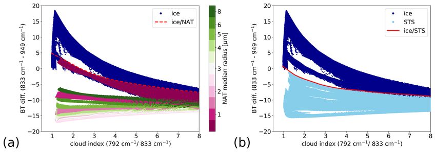
1898                                                    C. Kalicinsky et al.: Radiative transfer simulations of infrared spectra

different thicknesses of 1, 4, and 8 km, as in the case of bi-
modal NAT. Furthermore, we concentrated on the small and
medium-sized NAT particles up to 3.5 µm and used three dif-
ferent HNO3 VMRs of 5, 10, and 15 ppbv. We combined
these NAT scenarios with STS scenarios using 2/48 wt %,
volume densities of 5 and 10 µm3 cm−3 , and radii of 0.1, 0.3,
and 1.0 µm.
   The parameter ranges for all cloud scenarios are sum-
marised in Table 3, including the cloud extinction range. The
refractive indices for ice, NAT, and the STS mixtures were
taken from Toon et al. (1994), Biermann (1998) with refine-
ment in Höpfner et al. (2006), and Biermann et al. (2000) re-
spectively. The total number of scenarios was 16392 (NAT:             Figure 1. Selected simulation results for infrared spectra in the pres-
9240; STS: 3360; ice: 2352; and mixtures of bimodal NAT               ence of polar stratospheric clouds consisting of NAT particles with
and NAT–STS: 1440).                                                   different particle median radii, STS, and ice. The spectra have been
   Considering the computational resources required to sim-           scaled using the mean radiance in the 832.0–834.0 cm−1 (MW2)
ulate this number of scenarios, we assumed single scatter-            spectral window such that the radiance for all spectra equals one
ing. Neglecting multiple scattering introduces uncertainties.         in this window. The grey vertical bars mark the micro-windows
Based on the findings of Höpfner and Emde (2005) for our              (MWs) used during the analysis; they are numbered from MW1 to
optical depth ranges (Table 3, extinction times cloud thick-          MW7.
ness) and the single-scattering albedos of STS, NAT, and
ice, the uncertainty is mostly below 1 %, 4 %, and 4 % re-
spectively. However, for a few scenarios of 8 km thickness,           radiance in the 832.0–834.0 cm−1 spectral range is equal to
the uncertainty may reach up to 4.5 % for STS and 20 % for            one for all spectra. The example spectrum for the smallest
ice. In the cloud scenario set-up, we assumed homogeneous             median radius of 0.5 µm (yellow colour) exhibits a clear pro-
clouds. The horizontal extent of the CRISTA-NF line of sight          nounced peak at about 820 cm−1 . For slightly larger median
inside the PSC can reach up to several hundred kilometres.            radii (1.0–3.5 µm), the peak shifts to smaller wavenumbers
In the case of synoptic-scale PSCs, horizontal homogeneity            and becomes less pronounced (orange colours). When the
is a sufficiently good approximation. PSCs of other origin,           median radius is even larger, the spectral feature transforms
such as mountain-wave-induced PSCs, have a smaller hori-              to a step-like feature that shows a steep radiance decrease
zontal extent but are less frequent compared with synoptic-           from about 811 to 826 cm−1 . The magnitude of this decrease
scale PSCs.                                                           largely diminishes with increasing median radius.
                                                                         This behaviour and, thus, the dependency of the appear-
                                                                      ance of the feature on the median radius can be explained by
3     Results of the simulations                                      the different contributions of emission and scattering to the
                                                                      total observed radiance enhancement caused by the PSCs.
The following section deals with the analyses of the simu-            These contributions largely depend on the median radius of
lation results. The analyses can be divided into three parts:         the particles. The real and the imaginary part of the refrac-
(1) the shift in the NAT feature, (2) the detection of PSCs and       tive index of β-NAT are shown in Fig. 2a in black and red
the identification of the NAT and ice PSC types, and (3) the          respectively. The imaginary part illustrates the emission and
determination of the bottom altitude of the clouds.                   absorption characteristic of the NAT particles, whereas the
                                                                      real part shows the scattering behaviour. The imaginary part
3.1    Shift in the NAT feature                                       shows a distinct peak at about 820 cm−1 . As the emission is
                                                                      the major contribution when only small particles are present,
The appearance of the spectral feature that is observed in            the simulated spectra in the case of small NAT only show this
infrared limb spectra in the presence of polar stratospheric          peak. This is illustrated in Fig. 2b and c, where the extinction
clouds consisting of NAT particles in our study is unam-              and single-scattering albedo (SSA) are shown. The extinction
biguously characterised by the median radius of the particle          shows a clear peak at about 820 cm−1 , and the SSA, which
size distribution, as we kept the distribution width σ con-           gives the contribution of the scattering to the total extinc-
stant. With increasing median radius, the shape transforms            tion, shows low values. With increasing median radius of the
from the well-known pronounced peak at about 820 cm−1 to              NAT particles, the scattering becomes more and more im-
a peak that is slightly shifted towards smaller wavenumbers           portant. This can be seen by the increase in the SSA, which
and, finally, to a step-like feature. Figure 1 illustrates this be-   for large particles then can exceed 0.5, i.e. the scattering in-
haviour and the dependency of the appearance on the median            creasingly accounts for more than half of the total extinction.
radius. The spectra shown in Fig. 1 are scaled such that the          As a consequence, the peak shifts to smaller wavenumbers

Atmos. Meas. Tech., 14, 1893–1915, 2021                                                  https://doi.org/10.5194/amt-14-1893-2021
C. Kalicinsky et al.: Radiative transfer simulations of infrared spectra 1899
Table 3. Cloud scenario simulation set-up. Please note that “∗ ” refers to HNO3 VMR (ppbv), and “∗∗ ” refers to volume density (µm3 cm−3 ).
Cloud dimension Values
PSC position 13.0–30.0 km
PSC thickness 0.5, 1.0, 2.0, 4.0, 8.0 km
PSC type HNO3 VMR (ppbv)∗ / Radius (µm) Extinction (km−1 )
volume density (µm3 cm−3 )∗∗
NAT 1–15∗ 0.5, 1.0, 1.5, 2.0, 2.5, 3.0, 3.4 × 10⁻⁵ –2.2 × 10⁻³
3.5, 4.0, 5.0, 6.0, 8.0
Bimodal NAT 3/7, 5/5, 7/3∗ (first/second mode) First mode: 0.5–2.5 4.4 × 10⁻⁴ –1.4 × 10⁻³
Second mode: larger than in first mode
STS with H2 SO4 /HNO3 0.1, 0.5, 1.0, 5.0, 10.0∗∗ 0.1, 0.3, 0.5, 1.0 2.1 × 10⁻⁵ –4.1 × 10⁻³
2/48, 25/25, and 48/2 wt %
NAT + STS 2/48 wt % NAT: 5, 10, 15∗ NAT: 0.5–3.5 5 × 10⁻⁴ –3.5 × 10⁻³
STS: 5.0, 10.0∗∗ STS: 0.1, 0.3, 1.0
Ice 0.1, 0.5, 1.0, 5.0, 10.0, 50.0, 100.0∗∗ 1.0, 2.0, 3.0, 4.0, 5.0, 10.0 1.0 × 10⁻⁵ –1.0 × 10⁻²
with increasing particle size until it transforms to a step-like are marked with grey bars in Fig. 1. Additionally, all indices
signature (see Figs. 1 and 2b). are summarised in Table 4.
The spectral feature with all its versions in the 810– The detection of NAT particles inside clouds is based on
820 cm−1 region is a unique signature that only occurs in the characteristic spectral behaviour in the 810–820 cm−1 re-
the presence of NAT PSCs and will be used for the detection gion. In previous studies, a NAT index, the radiance ratio be-
of NAT PSCs. Other PSCs consisting of STS or ice do not tween the spectral region of the typical NAT feature (819–
show this feature, as shown in Fig. 1 using two examples in 821 cm−1 ) and the region of the CO2 peak (788–796 cm−1 ),
light blue (STS) and dark blue (ice). In contrast to the other was introduced to detect PSCs containing small NAT parti-
PSC types, ice shows the largest relative difference between cles (e.g Spang and Remedios, 2003; Höpfner et al., 2006;
the 832.0–834.0 cm−1 region and the second spectral range Spang et al., 2012, 2016, 2018). Here, we define the NAT
of our simulations (940–965 cm−1 ). Only NAT PSCs con- index-1 as the radiance ratio between the 819–821 cm−1
sisting of particles with very small radii (< 1.0 µm) can also (MW3) and 791–793 cm−1 (MW1) regions and use the same
achieve large differences. This spectral behaviour in the case smaller window in the region of the CO2 peak as for the CI.
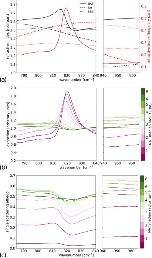
of ice will further be used to detect ice PSCs. In a scatter plot of the NAT index-1 versus the CI, we found
that spectra simulated for small NAT particles were separate
3.2 Detection of NAT from spectra simulated for larger NAT particles and other
types of PSCs (Fig. 3a). Note here that there is sometimes
3.2.1 Unimodal pure NAT an overlap of the data points for adjacent radii. This is also
the case in the other scatter plots. Nearly all simulations with
The detection of clouds using infrared limb spectra typically NAT particles < 3 µm lie above the region of the simulations
uses the cloud index (CI) (e.g Spang et al., 2001, 2002, 2008). for STS and ice clouds, which is marked by the solid red line.
The CI is the radiance ratio between a spectral region dom- The separation line was determined solely by the simulation
inated by CO2 at around 792 cm−1 and a second spectral results for ice and STS to define an upper limit of these simu-
region dominated by aerosol or cloud particles at around lations for each possible CI value. Thus, NAT particles within
833 cm−1 . For the analysis of the airborne observations by this size range can be detected and discriminated using NAT
CRISTA-NF, we used the 791.0–793.0 cm−1 (micro-window index-1.
MW1) and 832.0–834.0 cm−1 (MW2) windows. Because of In order to detect PSCs containing larger NAT particles
the different viewing geometries and instrument properties, and to make the estimation of the size range of the particles
the first window is defined with a smaller range than that more distinct, we introduce two new NAT indices here. The
typically used for satellite observations (Spang et al., 2008). NAT index-2, which is defined as the radiance ratio between
In cloud-free conditions, the CI value (MW1/MW2) is typi- 815–817 cm−1 (MW4) and 791–793 cm−1 (MW1), focuses
cally large (around 10). When clouds or larger aerosol loads on the shifted NAT feature that occurs for larger particles
are in the line of sight of the instrument, the CI significantly than that producing the non-shifted feature. Figure 3b shows
drops to smaller values depending on the optical thickness of the scatter plot of the NAT index-2 versus the CI. In contrast
the cloud. The MWs used for the CI and all following indices
https://doi.org/10.5194/amt-14-1893-2021 Atmos. Meas. Tech., 14, 1893–1915, 2021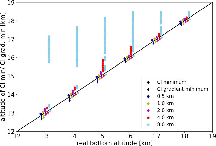
1900                                                       C. Kalicinsky et al.: Radiative transfer simulations of infrared spectra

Table 4. Summary of the indices and their corresponding micro-windows.

                      Name of index       Definition                                     Definition with short names
                      Cloud index CI      (791–793 cm−1 )/(832–834 cm−1 )                (MW1)/(MW2)
                      NAT index-1         (819–821 cm−1 )/(791–793 cm−1 )                (MW3)/(MW1)
                      NAT index-2         (815–817 cm−1 )/(791–793 cm−1 )                (MW4)/(MW1)
                      NAT index-3         (810–812 cm−1 )/(825–827 cm−1 )                (MW5)/(MW6)
                      BTD                 BT(832–834 cm−1 ) – BT(947.5–950.5 cm−1 )      BT(MW2) – BT(MW7)

                                                                         to the NAT index-1, the results for PSCs with larger NAT
                                                                         particles (up to 4 µm) now also lie above the simulations for
                                                                         STS and ice (red separation line). Additionally, for differ-
                                                                         ent particle median radii, the distance to the separation line
                                                                         changes when going from NAT index-1 to index-2 in an in-
                                                                         verse way. In the case of very small particles, the distance
                                                                         becomes smaller as the spectral region used for the detection
                                                                         moves away from the centre of the typical NAT peak. For
                                                                         larger particles, the opposite behaviour is observed, and the
                                                                         distance enlarges as the spectral region moves to the centre
                                                                         of the shifted NAT peak. This inverse behaviour can be seen
                                                                         in Fig. 3c, where the difference between NAT index-1 and
                                                                         index-2 is shown on the y axis. It is obvious that the simula-
                                                                         tions for the two smallest radii (0.5 and 1.0 µm) behave in an
                                                                         inverse manner to the simulations for larger radii.
                                                                            Lastly, we introduce the NAT index-3, which is defined as
                                                                         the radiance ratio between 810–812 cm−1 (MW5) and 825–
                                                                         827 cm−1 (MW6), to detect PSCs containing even larger
                                                                         NAT particles. This ratio enables the discrimination of a step-
                                                                         like feature from a peak and a more or less constant radi-
                                                                         ance in the complete spectral range as is the case for STS
                                                                         and ice. Figure 3d shows the scatter plot of the NAT index-3
                                                                         against the CI. The simulation results for small NAT particles
                                                                         (≤ 1.0 µm) have a NAT index-3 smaller than for the simula-
                                                                         tions results for STS and ice. A large part of the simulation
                                                                         results for larger NAT particles show a NAT index-3 that is
                                                                         larger than for the simulation results for STS and ice. By us-
                                                                         ing this ratio NAT particles with radii > 4 µm also separate
                                                                         from the other simulation results and are consequently de-
                                                                         tectable.
                                                                            In total, the three different NAT indices enable the de-
                                                                         tection of PSCs containing NAT particles and allow for a
                                                                         classification of the NAT particles in different size regimes.
                                                                         The detection and discrimination of NAT can be divided into
                                                                         three different cases: case 1 (small NAT) – NAT is detected
Figure 2. (a) Refractive indices for NAT (solid lines), STS (dotted      using the NAT index-1, and the difference NAT index-1 –
lines), and ice (dashed lines). The real parts are shown in black, and   index-2 is above the separation line; case 2 (medium NAT)
the imaginary parts are shown in red using the right y axis. The re-     – NAT is detected using the NAT index-2, and the differ-
fractive indices for NAT, STS, and ice were taken from Biermann          ence NAT index-1 – index-2 is below the separation line; and
(1998) with refinement in Höpfner et al. (2006), Biermann et al.
                                                                         case 3 (large NAT) – no detection of NAT using the NAT
(2000), and Toon et al. (1994) respectively. (b) Extinction spectra
for NAT with different median radii. The spectra have been scaled
                                                                         index-1 or index-2 (both below separation line), but the NAT
using the mean value in the 832.0–834.0 cm−1 spectral window             index-3 is above the separation line. Figure 4 shows the pro-
such that the extinction for all spectra equals one in this window.      portion between the spectra detected as being influence by
(c) Single-scattering albedo for NAT with different median radii.        NAT and the cloud spectra (spectra below a certain CI thresh-

Atmos. Meas. Tech., 14, 1893–1915, 2021                                                   https://doi.org/10.5194/amt-14-1893-2021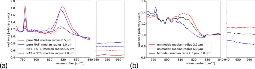
C. Kalicinsky et al.: Radiative transfer simulations of infrared spectra                                                                1901

Figure 3. Correlations between different NAT indices and the cloud index for the simulated PSC scenarios: (a) NAT index-1 (819–
821 cm−1 )/(791–793 cm−1 ); (b) NAT index-2 (815–817 cm−1 )/(791–793 cm−1 ); (c) NAT index-1 – NAT index-2; (d) NAT index-3 (810–
812 cm−1 )/(825–827 cm−1 ). The red lines show the separation lines, which mark the upper envelope of the regions of STS and ice defined by
the blue coloured areas (in panels a, b, and d) and the region of medium and large NAT with radii greater than 1.0 µm (in panel c). Simulation
results for ice and STS are in shown in dark and light blue respectively.

Figure 4. The histograms of the proportion of the detected spectra (NAT) per simulated cloud spectra in each size bin. The colours illustrate
the different cases (1–3): case 1 (sNAT) is shown in yellow, case 2 (mNAT) is shown in orange, and case 3 (lNAT) is shown in red. For a
description of the different cases, see the text. In panel (a), the CI threshold value to detect a spectrum as a cloud spectrum is 5.0 (about
365 000 cloud spectra in total), whereas the threshold in panel (b) is 3.0 (about 197 000 cloud spectra in total).

old) in each size bin of the simulations (0.5–8.0 µm), colour            sults in case 3 (yellow colour) all show median radii larger
coded for the three different cases. In Fig. 4a, only observa-           than or equal to 2.5 µm, whereby the radius 2.5 µm only oc-
tions with a CI below 5.0 are taken into account. Obviously,             curs in a very small amount. Thus, the different cases all rep-
in case 1 (yellow colour), only NAT particles with a median              resent a specific size regime with little or no overlap with the
radius of 0.5 or 1.0 µm are detected. The detection results in           other cases. Particularly the very small NAT particles (0.5
case 2 (orange colour) go from 1.5 up to 4.0 µm, and the re-             and 1.0 µm) can be completely distinguished from the parti-

https://doi.org/10.5194/amt-14-1893-2021                                                     Atmos. Meas. Tech., 14, 1893–1915, 2021
1902                                                   C. Kalicinsky et al.: Radiative transfer simulations of infrared spectra

cles with other median radii, as all of the detected spectra in     influence the analysis. Especially in the case of STS or ice,
this size range fall into case 1. The other two cases overlap       which show no distinct spectral features in the 810–820 cm−1
with each other.                                                    region, the data points in the scatter plots only slightly shift
   The total detection capacity with respect to the simulations     along the correlation lines or regions for the specific PSC
is also very good. For median radii up to 6.0 µm, nearly all        type. Thus, the separation lines, which are defined using the
spectra that have been detected as cloud spectra can be de-         STS and ice simulations (see Fig. 3), are still valid in such
tected as spectra influenced by NAT particles. However, a           cases. Consequently, a false detection by an assignment of
few cloud spectra cannot be identified as NAT spectra for           STS or ice to a NAT class is not possible. For NAT clouds, the
2.5 and 3.0 µm. These spectra all have a larger CI value            impact of underlying clouds slightly depends on the median
(> 3.0, optically thinner), and the separation between NAT          radius of the particles, as the scattering contribution increases
and the other PSC types degrades for larger CI values (see          with radius (see Fig. 2c). For median radii ≤ 1.0 µm, an in-
Fig. 3). Thus, a small part of the cloud spectra influenced by      fluence of a tropospheric cloud is negligible, as the spectra
NAT cannot be distinguished from STS and ice. When the              are dominated by absorption and emission. For larger me-
CI threshold value is reduced to 3.0, the detection itself and      dian radii a little change in the features can occur and a little
also the separation between the different size regimes im-          change in the positions of the data points in the scatter plots is
proves, as shown in Fig. 4b. Now all spectra for median radii       possible. Possible effects are an eventual assignment of NAT
up to 6.0 µm are identified as NAT. Additionally the sepa-          with a median radius of 1.5 µm to the class sNAT (upward
ration between the different sizes is now better, and case 3        shift in data points for the difference NAT index-1 – NAT
only detects radii ≥ 3.5 µm. Independent of the CI thresh-          index-2) or a missing detection for lNAT (downward shift
old value, only a part of the simulations for the largest me-       in data points for NAT index-3). Thus, a very small part of
dian radius of 8.0 µm are detected as NAT (CI < 5.0: ∼ 30 %;        the uncertainty in the class boundaries cannot be completely
CI < 3.0: ∼ 40 %). This is caused by the decreasing magni-          ruled out. However, the majority of all possible situations
tude of the radiance decrease from 811 to 826 cm−1 for an           will still be detected and classified correctly.
increasing median radius (see Sect. 3.1). The improvement
in the detection and discrimination when using a CI thresh-         3.2.3   Mixed NAT–STS clouds
old of 3.0 shows that it is not advisable to use a larger thresh-
old when analysing observations. According to the different         We additionally simulated mixed NAT–STS clouds to evalu-
size ranges of the three cases, the cases are hereafter denoted     ate the influence on the spectra and, specifically, the perfor-
as small NAT (sNAT: ≤ 1.0 µm), medium NAT (mNAT: 1.5–               mance of our classification into different size regimes. Here,
4.0 µm), and large NAT (lNAT: ≥ 3.5 µm). Compared with              we only simulated a subset of all possible combinations, as
the former method where only the NAT index-1 is used (e.g.          the spectral behaviour for each median radius is very simi-
Spang and Remedios, 2003; Höpfner et al., 2006; Spang               lar independent of factors such as the bottom altitude of the
et al., 2012, 2016, 2018), our new approach with three NAT          cloud or the thickness (see Sect. 2.4).
indices enables an improved detection capacity, as more NAT            If STS is present in addition to NAT, the relative mag-
clouds can be detected. For our simulations, the improvement        nitudes of the spectral features caused by NAT particles
is about a factor of 1.78 (approximately 190 000 cloud spec-        get smaller; therefore, the separation between these mixed
tra identified as NAT with all new indices and about 108 000        clouds and STS is also restricted compared with a pure NAT
spectra identified as NAT when only using index-1) for a            cloud. Figure 5a shows example spectra for PSCs of pure
CI < 3.0.                                                           NAT (solid lines in red for 0.5 µm and blue for 1.0 µm) and
                                                                    PSCs with the same NAT as well as STS (dashed lines) to
3.2.2   Influence of tropospheric clouds                            illustrate this effect. In a scatter plot of the NAT indices ver-
                                                                    sus the CI (compare Fig. 3a and b), the simulation results
The influence of tropospheric clouds was intensively stud-          for the NAT–STS mixtures are closer to the separation line
ied during the analysis of the radiative transfer simulations       or even below it compared with pure NAT. When the NAT
for various PSC situations for the MIPAS-Env satellite in-          detection and classification procedure (described in the pre-
strument (Spang et al., 2012, 2016), and the results can be         vious subsection) is applied to the simulation results for the
transferred to this study. A tropospheric cloud below the PSC       mixed clouds, the good discrimination between the small and
mainly influences the absolute radiance values where the            medium-sized particles remains. This discrimination relies
cold tropospheric cloud leads to lower overall radiance val-        on the difference in the NAT index-1 and index-2, where
ues. The appearance of the spectral signature (typical peak,        both indices are influenced in the same way. Therefore, the
shifted peak, or step-like behaviour) in the 810 to 820 cm−1        sign of the difference remains the same, because it depends
region remains nearly unchanged. Simulations by Woiwode             on the position of the spectral peak, which is not affected
et al. (2019) also showed these effects. As our detection           by the additional STS (see Fig. 5a). For a CI value below
method is based on colour ratios, i.e. relative effects, the        3.0, about 97.5 % of the simulated cloud spectra with median
change in the absolute radiance values does not significantly       radii of 0.5 and 1.0 µm are correctly detected as sNAT, and

Atmos. Meas. Tech., 14, 1893–1915, 2021                                               https://doi.org/10.5194/amt-14-1893-2021
C. Kalicinsky et al.: Radiative transfer simulations of infrared spectra 1903
Figure 5. Selected spectra for NAT–STS mixed clouds (a) and bimodal NAT particle size distributions (b). The spectra were scaled using
the mean radiance in the 832.0–834.0 cm−1 spectral window such that the radiance for all spectra equals one in this window. (a) The solid
lines show spectra for unimodal NAT particle size distributions. Red denotes a median radius of 0.5 µm and 10 ppbv HNO3 , and blue denotes
a median radius of 1.0 µm and 10 ppbv HNO3 . The dashed lines show the NAT–STS mixed clouds. The amount of NAT is the same as for
the pure NAT simulations, and the volume density of STS is 10 µm3 cm−3 in both cases. (b) The red and blue lines show the spectra for
unimodal size distributions with median radii of 2.5 and 6.0 µm respectively. The amount of HNO3 is 10 ppbv in each case. The black line
shows the simulation results for a bimodal size distribution with median radii of 2.5 and 6.0 µm and 5 ppbv HNO3 in each mode.
only about 0.3 % are incorrectly detected as mNAT (the re- or 30/70, the spectrum looks more like the spectrum for the
maining 2.2 % are not detected as NAT). In some cases STS unimodal size distribution that dominates the bimodal dis-
completely masks the spectral features caused by NAT, and tribution, because of more HNO3 in the corresponding size
NAT is not detectable any more. However, for a CI value be- range.
low 3.0, more than 90 % of the cloud spectra can still be iden- We also applied our classification procedure to these sim-
tified as containing NAT in the entire simulated size range. ulations for bimodal size distributions with the following re-
The proportion typically decreases with increasing median sults. When the first mode dominates (70 % HNO3 ), nearly
radius, i.e. more NAT-influenced spectra at 3.0 µm are missed all cloud spectra simulated for a median radius of 0.5 or
than at 0.5 µm, and will also decrease with increasing STS 1.0 µm are still detected as sNAT (about 99 % sNAT and
volume density or decreasing HNO3 VMR inside the PSC. 1 % mNAT) and, thus, classified correctly. All spectra that
In a nutshell, in mixed NAT–STS clouds, fewer scenarios are are identified as cloud (CI < 3.0) are also identified as NAT-
identified as containing NAT, because the STS reduces the containing PSCs. For a HNO3 ratio of 50/50 or 30/70, the
amplitude of the characteristic NAT signature. However, if a influence of the second mode increases such that more and
scenario in our simulations was classified as NAT, the size more spectra are detected as mNAT and a small part are de-
attribution remains as reliable as in the pure NAT scenarios. tected as lNAT. In the case of a 50/50 ratio, about 50.5 % are
classified as sNAT and 49.5 % are classified as mNAT; for a
3.2.4 Bimodal NAT clouds 30/70 ratio, 21 % are classified as sNAT, 77 % are classified
as mNAT, and 2 % are classified as lNAT. When combined
with larger NAT particles in the second mode (≥ 4 µm), a
In addition, we also simulated PSCs using bimodal NAT
part of the cloud spectra (CI < 3.0) are not detected as NAT
particle distributions with a main focus on the small and
because neither a spectral peak nor a step-like behaviour can
medium-sized particles and the separation between those.
be detected (50/50: 0.5 % and 30/70: 10 %). However, these
Here, a subset of all possible combinations was also simu-
cases are only a few percent of all cloud spectra in our sim-
lated (see Sect. 2.4).
ulations. When the first mode has a median radius between
The spectra simulated for the bimodal NAT particle size
1.5 and 2.5 µm, about 99 % of the simulated spectra are iden-
distributions are typically some kind of mixture of the spec-
tified as mNAT (1 % lNAT, when the median radius in the
tra for the corresponding unimodal distributions; thus, the
second mode is 5.0 or 6.0 µm) independent of the ratio of the
HNO3 VMR ratio plays an important role. Figure 5b shows
HNO3 VMRs. Furthermore, only a few spectra per thousand
an example of a spectrum simulated for a bimodal NAT par-
of those identified as clouds cannot be classified as NAT-
ticle distribution (black line). The HNO3 VMRs were 5 ppbv
containing PSCs. In total, our new classification scheme de-
in each mode with median radii of 2.5 and 6.0 µm. The two
livers very reasonable results even in the case of bimodal
corresponding spectra for the unimodal size distributions are
NAT particle size distributions.
shown in red and blue respectively. Obviously, the spectrum
for the bimodal size distribution is a mixture of the other two.
When the HNO3 ratio for both modes is changed to 70/30
https://doi.org/10.5194/amt-14-1893-2021 Atmos. Meas. Tech., 14, 1893–1915, 20211904 C. Kalicinsky et al.: Radiative transfer simulations of infrared spectra
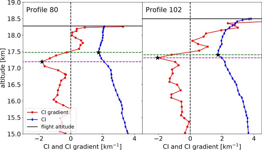
3.3 Detection of ice to determine the bottom altitude of the observed cloud. The
cloud index, which is used to detect optically thick conditions
The detection of ice uses the fact that a large radiance de- caused by clouds (or aerosol), shows characteristic vertical
crease from about 833 to 949 cm−1 can be observed in the changes in the presence of clouds. These changes are used
presence of ice (see Fig. 1). This clear decrease is only ob- for the detection of the cloud bottom altitude.
served in the case of ice or in the presence of very small Figure 7a shows examples of CI altitude profiles for clouds
NAT particles. Spang et al. (2012, 2016) used this spec- with different vertical thicknesses. When the complete cloud
tral behaviour to detect ice clouds in satellite measurements is located below the flight altitude (yellow colour), the CI
of MIPAS-Envisat. The authors used the brightness tem- largely drops to low values when entering the cloud from
perature (BT) difference between the two spectral regions. above (or slightly above because of the FOV). In the case
Here, we adopt the same method for the CRISTA-NF ob- that the flight altitude is inside the cloud, the CI is already
servations. Because of the different viewing geometry, spec- low at flight altitude. The CI then typically further decreases
tral resolution, and the different definition of the CI for the with decreasing altitude inside the cloud, and the minimum
two instruments, the separation lines have to be newly de- CI value is reached close to the bottom altitude. In some
fined. The spectral regions used for the BT difference are cases, when the vertical thickness is larger (4 km or 8 km),
832.0–834.0 cm−1 (MW2) and 947.5–950.5 cm−1 (MW7). the CI minimum can be located somewhere inside the cloud.
In a scatter plot of the BT difference against the CI, the sim- When leaving the cloud, the CI increases again. These verti-
ulated ice spectra clearly separate from other particle types cal changes in the CI can be best illustrated with the gradient
(Fig. 6). Obviously, spectra that are influenced by ice clearly of the CI (Fig. 7b). Slightly above the cloud top, the verti-
separate from STS and nearly all NAT particles when the cal gradient maximises, and slightly below the cloud bottom,
cloud is optically thick enough (low CI). For larger CI, values the gradient reaches its minimum value. In contrast to the CI
the separation becomes smaller. The only particles that can minimum, where larger deviations from the cloud bottom can
produce similar values of the BT difference are very small occur, the minimum of the gradient is always slightly below
NAT particles with median radii of 0.5 µm (yellow colours the real bottom altitude of the cloud.
in Fig. 6a), but these particles can be safely filtered out us- Figure 8 summarises the results for the simulated clouds
ing the method described in Sect. 3.2. Consequently, the BT with a bottom altitude below flight altitude. In the case of the
difference is a very robust method to detect ice particles in CI minima (full circles), there are sometimes larger devia-
PSCs. tions from the real bottom altitude when the cloud is verti-
cally thick (red and light blue full circles). The CI gradient
3.4 Detection of STS minima (full diamonds) are always located close to the real
bottom altitude, at the first or the second measurement below.
The spectra for STS show neither a local spectral feature like The possibility to observe the gradient minimum at the sec-
the spectra for NAT nor a broadband spectral feature such ond measurement below the cloud increases with decreasing
as the spectra for ice. Thus, the detection of STS can not be altitude of the cloud, because the vertical extent of the FOV
achieved by using a unique spectral behaviour. In practice, (in metres) is larger at lower altitudes. In our simulations, this
the detection procedure is as follows. Firstly, the NAT detec- occurs only at bottom altitudes of 13.0 and 14.0 km. In sum-
tion methods are used to detect observations of NAT particles mary, the CI minimum and the gradient minimum enclose
and to distinguish between the three size regimes. Secondly, the real bottom altitude. A large gap between the two mini-
the BT difference method is applied to the observations to mum values indicates the observation of a cloud with a larger
detect ice. Finally, the observations inside PSCs that are nei- vertical thickness.
ther detected as NAT nor as ice are categorised as STS. It is There are further restrictions on the determination of the
not necessarily the case that the spectra categorised as STS bottom altitude. In some cases, the observations run into sat-
are solely influenced by STS; it is possible that NAT or ice uration, and the CI values below the cloud bottom altitude
were also present in the PSC, but the additional amount of converge at a low value. Additionally, in other situations,
STS was enough to minimise the spectral features such that the CI values below the bottom altitude only show a linear
NAT or ice was no longer definitely detectable. Furthermore, increase and not the larger change directly below the bot-
the small amount of very large NAT particles that cannot be tom altitude. In both cases, the CI minimum and the gradi-
distinguished from STS and ice will also fall into the STS ent minimum cannot sufficiently be determined and used for
category. the detection of the bottom altitude of the cloud. An effec-
tive way to sort out observations that are possibly affected
3.5 Bottom altitude of the PSCs is the use of a threshold value. We derived a CI minimum
below 1.25 from the simulations. Such low CI values only
Further important quantities with respect to cloud detection occur for a part of the ice clouds simulated here (typically
are the vertical thickness and the position of the cloud defined for largest volume densities of 50 and 100 µm3 cm−3 ; with
by the top and bottom altitude. Here, we present a method increasing vertical thickness, some simulations with 5 and
Atmos. Meas. Tech., 14, 1893–1915, 2021 https://doi.org/10.5194/amt-14-1893-2021You can also read