Implementation of the swLORETA in a Cloud Based Service for EEG Analysis - VIGNESH NANDAGOPAL
←
→
Page content transcription
If your browser does not render page correctly, please read the page content below
Implementation of the swLORETA in a
Cloud Based Service for EEG Analysis

VIGNESH NANDAGOPAL

DEPARTMENT OF ELECTRICAL ENGINEERING
C HALMERS U NIVERSITY     OF   T ECHNOLOGY
Gothenburg, Sweden 2021
www.chalmers.se
Master’s thesis 2021

Implementation of the swLORETA in a cloud
      based service for EEG Analysis

                Vignesh Nandagopal

          Department of Electrical Engineering
                Biomedical Engineering
        Chalmers University of Technology
               Gothenburg, Sweden 2021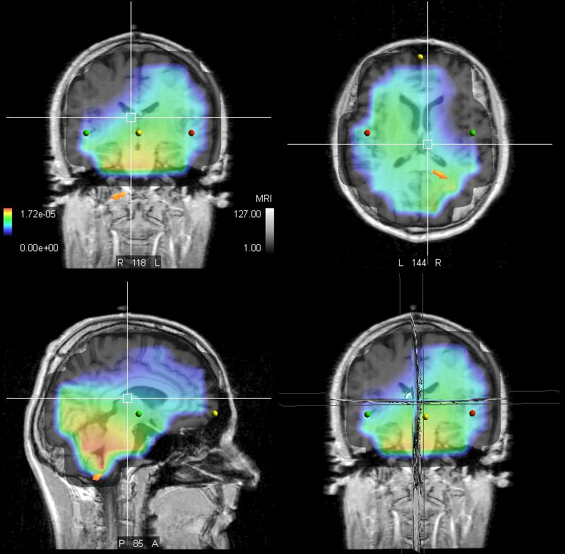
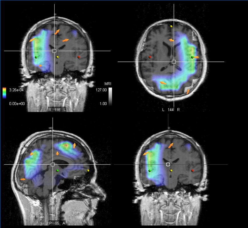
Implementation of the swLORETA in a cloud based service for EEG Analysis
Vignesh Nandagopal

© Vignesh Nandagopal, 2021.

Supervisor: Ralf Hauffe, eemagine Medical Imaging Solutions GmbH
Examiner: Fredrik Brännström, Communication Systems, Electrical Engineering

Master’s Thesis 2021
Department of Electrical Engineering
Division of Signals and System
Chalmers University of Technology
SE-412 96 Gothenburg
Telephone +46 31 772 1000

Cover: Source localization using the swLORETA algorithm in a three head di-
mensional model. The points indicate positions within the brain that have been
activated.

Typeset in LATEX, template by Magnus Gustaver
Gothenburg, Sweden 2021

iv
Implementation of the swLORETA in a cloud based service for EEG
Analysis
Vignesh Nandagopal
Department of Electrical Engineering
Chalmers University of Technology

Abstract
Electroencephalography is a diagnostic technique that records the brain’s sponta-
neous electrical activity. Once the recording is received, source localization is per-
formed, which facilitates identifying the key areas of the brain responsible for the
signal. The issue with electroencephalography is that the instrument takes up a lot
of room and the analysis segments are desktop cpu intensive tasks. In this thesis,
we investigate at how contemporary cloud computing solutions can be used to build
swLORETA, a source localization technique. The electroencephalography becomes
more robust with the fundamental deployment of a cloud computing setup with a
microservice architecture. The source localization approach produces identical find-
ings to the traditional desktop machine arrangement and visualized in a magnetic
resonance image. This configuration opens the way for more appealing electroen-
cephalography and other healthcare-related diagnostic solutions in the future.

Keywords: EEG, source localization, swLORETA, cloud computing

                                                                                    v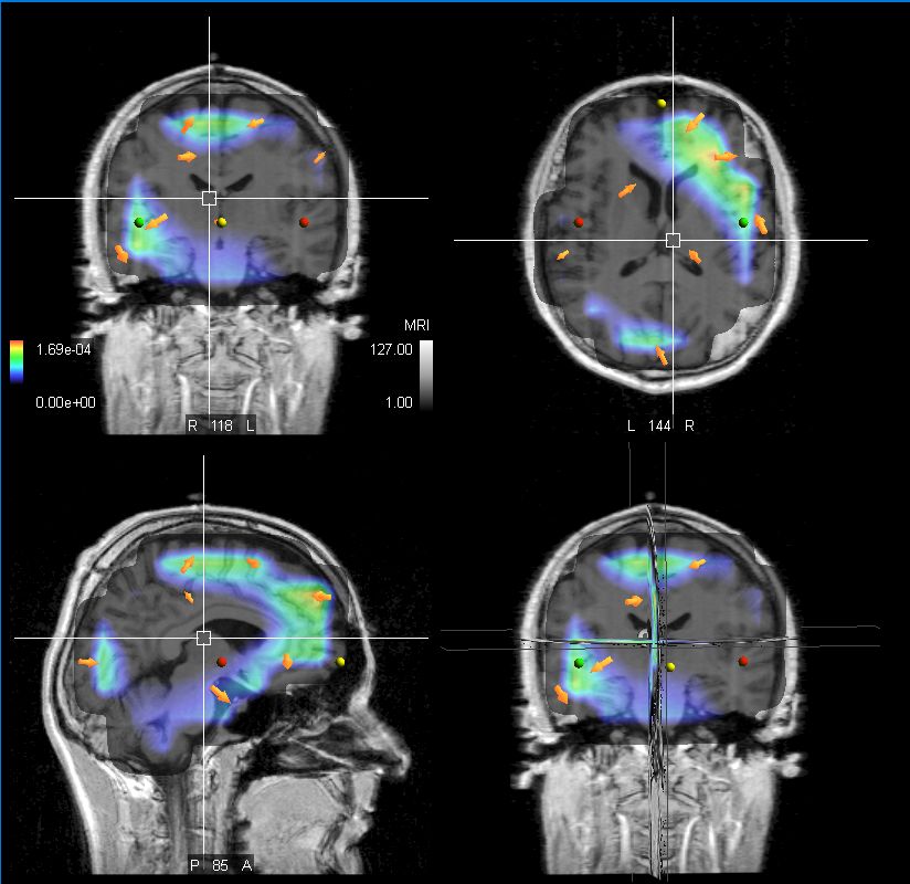
Acknowledgements
First and foremost, I’d like to thank Yibo Wu, my thesis advisor, and Fredrik
Brännström, the examiner from Chalmers University of Technology’s Electrical En-
gineering Department. They have always been willing to assist me with any ques-
tions I had about my thesis. I’d want to express my gratitude to the Chalmers
University of Technology for providing the high-quality education they promised.

I would like to express my heartfelt gratitude to Ralf Hauffe and Frank Zanow of
eemagine Medical Imaging Solutions GmbH for entrusting me with this opportunity.
I’d also like to thank Jacob Kanev for his unwavering support throughout our thesis
discussions, as well as for his advice and insight.

I’d also like to thank my parents, who have been a rock of support throughout this
challenging time.

                                     Vignesh Nandagopal, Gothenburg, June 2021

                                                                                vii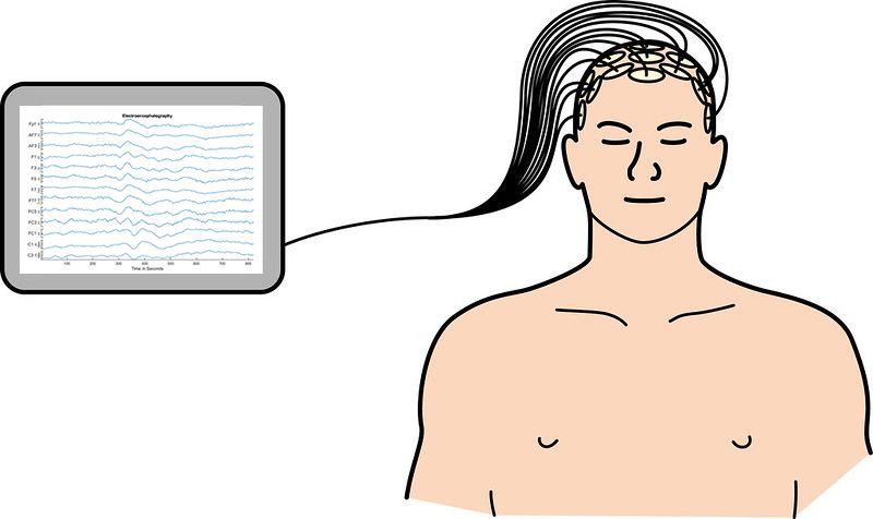
Contents

List of Figures                                                                                                                               xi

List of Abbreviations                                                                                                                        xiii

1 Introduction                                                                                                                                 1
  1.1 Purpose and Goal .     .   .   .   .   .   .   .   .   .   .   .   .   .   .   .   .   .   .   .   .   .   .   .   .   .   .   .   .     2
  1.2 Research Questions     .   .   .   .   .   .   .   .   .   .   .   .   .   .   .   .   .   .   .   .   .   .   .   .   .   .   .   .     2
  1.3 Limitation . . . . .   .   .   .   .   .   .   .   .   .   .   .   .   .   .   .   .   .   .   .   .   .   .   .   .   .   .   .   .     2
  1.4 Related Work . . .     .   .   .   .   .   .   .   .   .   .   .   .   .   .   .   .   .   .   .   .   .   .   .   .   .   .   .   .     3

2 Theory                                                                                                                                       5
  2.1 What is EEG? . . . . . . . . . . . . . . . . . . . .                                       .   .   .   .   .   .   .   .   .   .   .     5
      2.1.1 EEG Signals in the Human Body . . . . .                                              .   .   .   .   .   .   .   .   .   .   .     5
  2.2 Characteristics of EEG signals . . . . . . . . . . .                                       .   .   .   .   .   .   .   .   .   .   .     7
  2.3 Acquiring EEG signals . . . . . . . . . . . . . . .                                        .   .   .   .   .   .   .   .   .   .   .     8
      2.3.1 EEG Setup . . . . . . . . . . . . . . . . .                                          .   .   .   .   .   .   .   .   .   .   .    10
      2.3.2 Noise and Factors Affecting to EEG Signal                                            .   .   .   .   .   .   .   .   .   .   .    11
      2.3.3 Mathematical Representation of EEG . . .                                             .   .   .   .   .   .   .   .   .   .   .    12
  2.4 Magnetic Resonance Imaging . . . . . . . . . . .                                           .   .   .   .   .   .   .   .   .   .   .    12
  2.5 EEG Forward Model . . . . . . . . . . . . . . . .                                          .   .   .   .   .   .   .   .   .   .   .    13
      2.5.1 Dipoles . . . . . . . . . . . . . . . . . . . .                                      .   .   .   .   .   .   .   .   .   .   .    15
      2.5.2 Algebraic Formulation . . . . . . . . . . .                                          .   .   .   .   .   .   .   .   .   .   .    16
  2.6 EEG Inverse Model . . . . . . . . . . . . . . . . .                                        .   .   .   .   .   .   .   .   .   .   .    17
      2.6.1 Generalized Cross Validation . . . . . . . .                                         .   .   .   .   .   .   .   .   .   .   .    19
      2.6.2 sLORETA . . . . . . . . . . . . . . . . . .                                          .   .   .   .   .   .   .   .   .   .   .    19
  2.7 Singular Value Decomposition . . . . . . . . . . .                                         .   .   .   .   .   .   .   .   .   .   .    20
      2.7.1 swLORETA . . . . . . . . . . . . . . . . .                                           .   .   .   .   .   .   .   .   .   .   .    20
  2.8 Head Models and Leadfield Matrix . . . . . . . .                                           .   .   .   .   .   .   .   .   .   .   .    21

3 Methods                                                                                                                                     23
  3.1 swLORETA Algorithm . . . . .                       .   .   .   .   .   .   .   .   .   .   .   .   .   .   .   .   .   .   .   .   .    23
  3.2 Cloud Computing . . . . . . . .                    .   .   .   .   .   .   .   .   .   .   .   .   .   .   .   .   .   .   .   .   .    23
  3.3 Setup Proposed . . . . . . . . .                   .   .   .   .   .   .   .   .   .   .   .   .   .   .   .   .   .   .   .   .   .    25
      3.3.1 The Cloud Setup . . . .                      .   .   .   .   .   .   .   .   .   .   .   .   .   .   .   .   .   .   .   .   .    25
      3.3.2 Algorithm in the Cloud .                     .   .   .   .   .   .   .   .   .   .   .   .   .   .   .   .   .   .   .   .   .    26
      3.3.3 Setting up the Solution .                    .   .   .   .   .   .   .   .   .   .   .   .   .   .   .   .   .   .   .   .   .    27
  3.4 Leadfield Matrix . . . . . . . .                   .   .   .   .   .   .   .   .   .   .   .   .   .   .   .   .   .   .   .   .   .    27

                                                                                                                                              ix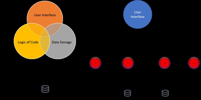
Contents

    3.5   Solution Visualization . . . . . . . . . . . . . . . . . . . . . . . . . . 28
    3.6   Datasets . . . . . . . . . . . . . . . . . . . . . . . . . . . . . . . . . . 28

4 Results                                                                                                     29
  4.1 Solution Architecture . . . . . . . . . . . . . . .     .   .   .   .   .   .   .   .   .   .   .   .   29
      4.1.1 Working of the Solution . . . . . . . . .         .   .   .   .   .   .   .   .   .   .   .   .   29
  4.2 Performance . . . . . . . . . . . . . . . . . . . .     .   .   .   .   .   .   .   .   .   .   .   .   30
      4.2.1 Performance of Cloud Setup . . . . . . .          .   .   .   .   .   .   .   .   .   .   .   .   30
      4.2.2 Comparison between Cloud and Desktop              .   .   .   .   .   .   .   .   .   .   .   .   31
  4.3 Solution Visualization . . . . . . . . . . . . . .      .   .   .   .   .   .   .   .   .   .   .   .   32
  4.4 Future Possibilities . . . . . . . . . . . . . . . .    .   .   .   .   .   .   .   .   .   .   .   .   36

5 Conclusion                                                                                                  39

Bibliography                                                                                                  41

x
List of Figures
2.1 A simple illustration a multiple channel EEG collecting data using
electrodes from multiple locations across the scalp of a human being.
The image has been modified from [10]. CC BY-NC-ND 2.0 . . . . . 6
2.2 An illustration of a neuron which is the basic building block of the
brain [15]. CC BY-SA 4.0. . . . . . . . . . . . . . . . . . . . . . . . 7
2.3 An illustration of the different brain waves and a description of what
activities would be associated with these brain waves. CC0 1.0. . . . 8
2.4 Example of a signle channel EEG recording which represents the dif-
ferential amplification between active and reference electrode. The
voltage is on the y-axis and time is in the x-axis. . . . . . . . . . . . . 9
2.5 An illustration of the 10-20 electrode positioning standard followed
for EEG. This image has been Released to Public Domain. . . . . . . 10
2.6 A simple circuit diagram explaining the EEG setup similar. . . . . . . 11
2.7 An example of an MRI of the head section. This image is a T1-
weighted MRI scan. The following are the basic orientation terms, a
coronal plane from the front which is seen on the top left, a sagittal
plane that is seen from the side which is in the bottom left and trans-
verse plane observed from the top down which is seen on the right
side of the image. . . . . . . . . . . . . . . . . . . . . . . . . . . . . . 13
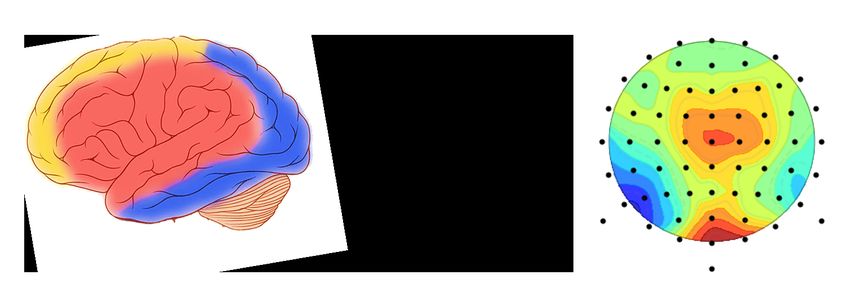
2.8 An illustration of the forward model which means calculating the
EEG electrode potentials from knowing the values of distribution
of current source density in the brain. The left side of the image
shows the activation maps of the brain, while the right side shows a
schematic of the head with EEG electrodes shown as black dots and
their potential values. The image has been modified from [30]. CC
BY-SA 3.0. . . . . . . . . . . . . . . . . . . . . . . . . . . . . . . . . 14
2.9 An example of the EEG inverse model where the current source den-
sity, that is induced by dipoles that are spread across the brain is
estimated using the EEG electrode potentials. The left side of the
image shows the activation maps of the brain, while the right side
shows a schematic of the head with EEG electrodes shown as black
dots and their potential values. The image has been modified from
[30]. CC BY-SA 3.0. . . . . . . . . . . . . . . . . . . . . . . . . . . . 17
xiList of Figures
3.1 An example of monolithic architecture where all services are combined
into one setup is depicted on the left and a microservice architecture
for cloud computing which has a separate container performing indi-
vidual operations is depicted on the right side. . . . . . . . . . . . . . 24
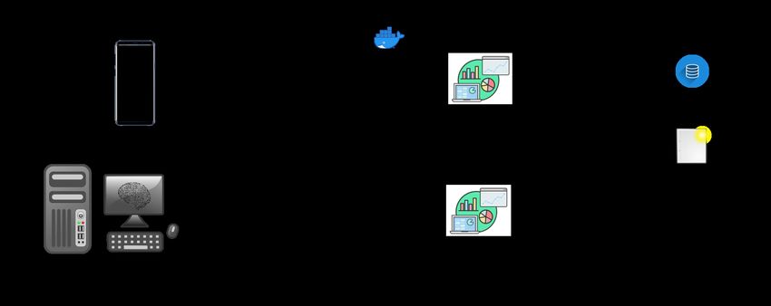
3.2 An example of the how the cloud is used is EEG source analysis. . . . 25
3.3 swLORETA Algorithm that has been implemented in the cloud. . . 26
4.1 The software architecture used in setting up the cloud computing
solution of swLORETA. The architecture used follows a microservice
architecture. . . . . . . . . . . . . . . . . . . . . . . . . . . . . . . . . 30
4.2 The performance time of the source localization method using the
cloud application tested with the 64 Channel EEG setup. . . . . . . 31
4.3 The performance time of the source localization method using the
cloud application tested with the 32 and 20 Channel EEG setup. . . 32
4.4 A comparison between the time taken for the source localization re-
sults using the swLORETA algorithm in the desktop machine and
cloud setup is compared. . . . . . . . . . . . . . . . . . . . . . . . . . 33
4.5 The swLORETA result that has been overlaid on MRI scan for a
64 Channel Montage. The arrows in the image point towards the
activation maps in the brain. The blue activation maps express mini-
mal intensity, fluorescent to yellow symbolises a moderate amount of
activity, and red maps designate the maximum intensity of current
density. The yellow dot indicates the nasion point of the head, and
the red dot indicates the left ear, and the green dot indicates the right
ear, respectively. These points are used for reference to read the MRI
concerning how the head is oriented. . . . . . . . . . . . . . . . . . . 34
4.6 The swLORETA result that has been overlaid on MRI scan for a
32 Channel Montage. The arrows in the image point towards the
activation maps in the brain.The blue activation maps express mini-
mal intensity, fluorescent to yellow symbolises a moderate amount of
activity, and red maps designate the maximum intensity of current
density. The yellow dot indicates the nasion point of the head, and
the red dot indicates the left ear, and the green dot indicates the right
ear, respectively. These points are used for reference to read the MRI
concerning how the head is oriented. . . . . . . . . . . . . . . . . . . 35
4.7 The swLORETA result has been overlaid on an MRI scan for a 20
Channel Montage. The arrows in the image point towards the acti-
vation maps in the brain. The blue activation maps indicate minimal
intensity, flourescent to yellow indicates a moderate amount of ac-
tivity and red maps indicate maximum intensity of current density.
The yellow dot indicates the nasion point of the head, the green dot
indicates the left ear and the green dot indicates the right ear re-
spectively. These points are used for reference to read the MRI with
respect to how the head is oriented. . . . . . . . . . . . . . . . . . . . 36
xiiList of Abbreviations
EEG Electroencephalography
swLORETA standardized weighted Low Resolution Tomography
sLORETA standardized Low Resolution Tomography
SVD singular value decomposition
MRI Magnetic resonance imaging
AP action potential
PSP postsynaptic potential
GCV Generalized Cross Validation
ECD Equivalent Current Dipole
PAN PreAuricular and Nasion
DICOM Digital Imaging and Communications in Medicine
xiiiList of Figures xiv
1
                           Introduction

Since the invention of the microprocessor, modern technology has moved towards
more compact technologies. Computers, mobile phones, and televisions have ben-
efitted from such changes and have become portable. This trend has now spread
to the medical field. The size of devices has reduced dramatically in recent years,
while the computational capacity of all of these devices has improved while keep-
ing a compact footprint [1]. These adjustments have also begun to benefit the
Electroencephalography (EEG). Recording of the spontaneous electrical activity of
the brain is called EEG. EEG systems with higher channel capacity take up more
space. However, amplifiers used in EEGs have reduced to a very compact size in
recent years [2].

In general EEG systems are connected to a desktop computer which provides a vi-
sual stimulus at regular time intervals while recording the signals. Thereby leading
the old EEG setup to occupy a larger space [2]. With the upcoming improvements
in handheld smartphone devices, it is possible to connect an EEG with a smart-
phone and start EEG recordings, thereby creating a possibility of shrinking the
entire setup. The following stage is to observe and analyze EEG recording utiliz-
ing Web applications and cloud-based services that can be accessed from anyplace
and eliminate the requirement for a high-powered desktop computer. Such advance-
ments benefit the overall medical diagnostics structure. The ability to conduct EEG
recordings at home will become increasingly common in the future. The more these
types of setups there are, the easier it is to do an EEG recording. The cloud com-
puting technique allows for faster machine learning-based observations on EEG data
as well.

This thesis focuses on analyzing these EEG signals in a cloud-based service, es-
pecially on source localization. Source localization of active sources in the brain
through EEG signals is a method of brain imaging utilized in a diversity of applica-
tions such as investigation of localized epilepsy and attention-deficit/hyperactivity
disorder [3].

The thesis is done in collaboration with eemagine Medical Imaging Solutions. They
provide complete end to end solutions for medical diagnostics by integrating different
modalities such as EEG, Magnetic resonance imaging (MRI), transcranial magnetic
stimulation and near-infrared spectroscopy.

                                                                                    1
1. Introduction
1.1 Purpose and Goal
The original plan for the thesis was to use machine learning or deep learning to
do source localization. Machine learning algorithms require massive volumes of
data. The problem with EEG recordings is that publicly available datasets are
low in number, and specifics on the visual stimulus utilized are not provided. The
product’s overall goal is to make large databanks available for EEG recordings in
the future, which can use machine learning or deep learning algorithms.
The goal of this thesis is to implement source localization in a cloud-based frame-
work using the standardized weighted Low Resolution Tomography (swLORETA)
algorithm. The technique will visualize the source localization in an averaged MRI
image using 20, 32, and 64 channel EEG measurements. The implementation of the
thesis work is done in C# programming language. The algorithm is deployed in the
cloud using the Docker framework to containerize the implementation. The cloud
application will provide the values of source localization when invoked, and a visu-
alization of this is done on an MRI. The solution presented utilizes a basic program
that is connected to the internet. It selects the EEG recording, invokes the cloud
setup, and the visualization of the EEG occurs. The source localization solution is
not an accurate representation of a person’s ideal source localization because we are
using an averaged MRI for our calculation purposes.
The goals of the master thesis is to :
• Study about EEG and their usage.
• Study about the various inverse solutions used in EEG.
• Study the swLORETA algorithm and implement the algorithm.
• Implement the source localization algorithm within a cloud framework
• Visualise the algorithm and how it works with various EEG channels.
1.2 Research Questions
With the mentioned purpose and goals it is important to formulate a few research
questions to answer through the results of thesis. The questions would be the
following,
• How to implement the algorithm swLORETA?
• How does the algorithm work as a cloud service and what is the architecture
we can use ?
• What are the differences in the solution when using it in a standalone system
in comparison with a cloud service?
1.3 Limitation
The implemented solution of source localization is essentially analytical. When at-
tempting to reproduce the swLORETA algorithm, numerous assumptions are made
21. Introduction
when attempting to reproduce this algorithm. The method cannot be utilized pri-
marily for direct surgical treatments, which would require individual MRI segmen-
tation [4]. It should be noted that EEG recordings have a low signal-to-noise ratio,
and where noise can come from a variety of sources, which could be a problem when
analyzing such solutions [5].
Furthermore, it is up to the company to maximize reliability and integrate the
project into future applications. When incorporating such features into its products,
the organization would devote additional time to product development. Companies
work hard to meet product milestones, and such features are likely to appear in
future product releases.
1.4 Related Work
Considerable research has been done in the past with regards to source localization
algorithms. EEG source localization algorithms are mainly divided into two sec-
tions, the parametric and non-parametric approach [6, 7]. Ernesto Palmero-Soler
et al. [7] proposed the swLORETA algorithm . The swLORETA algorithm’s over-
all resolution is improved by building on the previous standardized Low Resolution
Tomography (sLORETA) technique by introducing a singular value decomposition-
based lead field weighting method [7, 8]. As a result, the swLORETA method
outperforms the sLORETA algorithm in the presence of noise.
The fundamental disadvantage of the source localization approach is that it is com-
putationally expensive due to the inversion of large matrices. Basic desktop con-
figurations may take longer than expected to finish the computations and present
the results. This issue can be addressed by implementing the cloud computing tech-
nology presented in the thesis. This cloud-based EEG service would be the first of
its kind in the health industry. This could pave the way for future medical tests
that are more cost effective. This innovation can be seen very soon available in the
medical field. If the implementation is successful in products, more analysis tools
can be configured in the cloud.
31. Introduction 4
2
Theory
2.1 What is EEG?
An EEG is a recording of the flow of neuronal ionic currents through a pair of
electrodes positioned within or on the exterior of the scalp. The intracranial EEG
(iEEG) is acquired inside the scalp and is for surgical planning. Specifically, through-
out this thesis, the term “EEG” refers to an EEG recorded noninvasively with a
combination of electrodes attached to the scalp surface [9].
In the below Figure 2.1, an EEG recording is illustrated. A multiple channel EEG
is used and the recorded signal can be seen on the left side of the illustration. EEG
recordings is the one of the most efficient techniques to study the electrical activity
of the brain [11]. Within fractions of a second after a stimulus is applied, complex
patterns of brain activity can be recorded. When compared to an MRI and positron
emission tomography, EEG has inferior spatial resolution [12]. Thus, EEG pictures
are frequently coupled with MRI scans for better allocation within the brain. The
relative intensity and location of electrical activity in various brain areas may be
determined using EEG.
Generally, EEG is used in health care to [12]
• Detect awareness, coma, and brain death.
• Determining regions of damage caused by a seizures, head injury, stroke, tu-
mor, etc.
• Overall assessment of the cognitive activity.
• Regulate the depth of anaesthesia.
• Drugs are tested for violent effects.
• Detect sleep problems and physiology.
A simple EEG system incorporates EEG electrodes with conductive material or
electrolytic paste, an amplifier comprising filters, an analog to digital converter
coupled to a recording device, which is currently a desktop computer system, and a
monitor for visualizing the EEG recorded [12].
2.1.1 EEG Signals in the Human Body
The human brain is considered the most complex organ in the body. The brain
can be divided into the frontal, occipital, temporal, and parietal lobes. The four
lobes have various places and roles that support the human body’s responses and
behaviours [13].
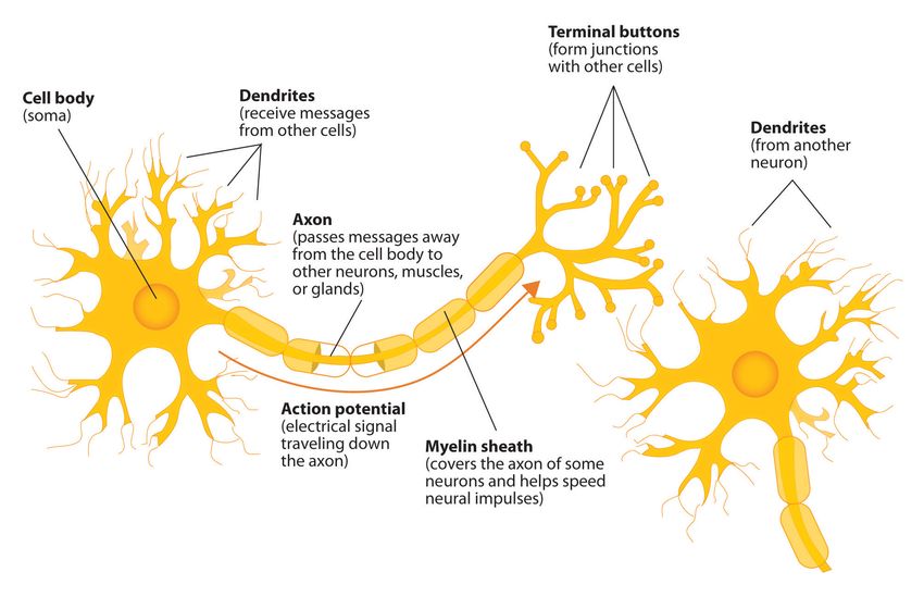
52. Theory Figure 2.1: A simple illustration a multiple channel EEG collecting data using electrodes from multiple locations across the scalp of a human being. The image has been modified from [10]. CC BY-NC-ND 2.0 Neurons are the basic building blocks of the brain and nervous system. They are the cells responsible for accumulating sensory information from the outside world, transmitting motor instructions to our muscles, and processing and relaying electri- cal impulses [14]. In Figure 2.2 an illustration of a neuron can be seen. The cell nucleus is the heart of the neuron, relaying instructions to the cell. The axon is a long, thin part of the neuron that binds its nucleus to the dendrite of another [11]. The dendrite is a tiny component of the neuron that contains numerous receptor sites for neurotransmitters provided by an axon terminal. Dendrites can grow on either one or both ends of the cell. An action potential (AP) is a mechanism in which an ion pumps along the exterior of an axon, rapidly alters its ionic composition and allows an electrical signal to pass immediately down the axon to the next dendrite [16]. As a result of this instant transition in ionic charge, a voltage is produced on both the inside and outside of the neuron’s cell membrane [17, 18]. These neurons produce chemicals known as neurotransmitters. Neuronal electrical activity may be classified into two categories: AP and postsynaptic potential (PSP). If the PSP exceeds the postsynaptic neuron’s threshold conduction level, the neuron fires and an AP is launched [11]. The EEG is assumed to be pro- duced predominantly by cortical pyramidal neurons in the cerebral cortex that are aligned perpendicular to the brain’s surface. The EEG that is detected is the sum of excitatory and inhibitory PSP from significantly large groups of neurons firing in a synchronized manner [19]. The PSP is unidirectional and is modeled as an equivalent current dipole. These PSPs are primary currents that cause extracellular currents to travel to the furthest reaches of the human body. The movement of these secondary currents via the scalp 6
2. Theory
Figure 2.2: An illustration of a neuron which is the basic building block of the brain [15]. CC
BY-SA 4.0.
generates a potential difference between two distant places over time, which results
in the EEG signal [20].
2.2 Characteristics of EEG signals
One of the most critical elements for evaluating abnormalities in clinical EEGs and
interpreting functional behaviors in cognitive research is frequency which is defined
as the number of cycles per second. Human EEG potentials are characterized as ape-
riodic unpredictable oscillations with irregular bouts of oscillations, having billions
of oscillating communities of neurons as its source [11]. When healthy individuals
shift between states, such as alertness and sleep, the amplitudes and frequencies of
such signals change.
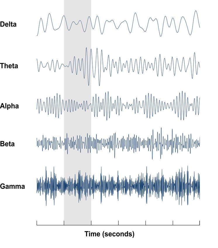
EEG signals have a frequency range of 0.01 Hz to approximately 100 Hz, which are
separated into five frequency bands. They are categorized as delta (δ), theta (θ),
alpha (α), beta (β) and gamma (γ) waves [21]. An illustration of these waves can be
seen in Figure 2.3. The delta wave has a frequency range up to 4 Hz, is characterized
by the largest amplitudes varying between 100µV to 200µV and has the slowest
wave speed. Deep sleep, major brain illnesses, and waking state are all linked to
it. The theta wave has a frequency of 4 to 8 Hz and amplitude between 50µV
to 100µV [11]. Emotional tension, particularly dissatisfaction or disappointment,
creative inspiration, as well as a profound meditation, all trigger theta. The alpha
wave has a frequency range between 8 to 13 Hz with a 30–50 µV amplitude, and
it is predominantly found in the brain’s posterior parts. The alphas waves are best
captured when the patient’s eyes are closed or when they are calm. It is frequently
72. Theory Figure 2.3: An illustration of the different brain waves and a description of what activities would be associated with these brain waves. CC0 1.0. linked to high levels of mental activity, stress, and tension. The beta wave oscillates between 13 to 30 Hz. It emerges uniformly on both sides in the frontal region, with a small amplitude and fluctuating frequency. Beta waves are produced when the brain is stimulated and actively engaged in mental activity [11]. These waves indicate higher levels of engagement in the mind. The beta wave is a type of brain wave that is connected with performing activities, paying attention, and focusing on critical challenges. The frequency of gamma waves ranges from 30 Hz and upwards. The maximum frequency of this rhythm is frequently described as being approximately 80 or 100 Hz. It’s linked to a variety of cognitive and motor processes. Beyond these frequencies if anything appears these can indicate the onset of epileptic seizures. 2.3 Acquiring EEG signals Voltages are graphed vertically and time is graphed horizontally in a typical EEG display, producing a near real-time display of ongoing cerebral activity. EEG em- ploys the theory of differential amplification, or recording voltage changes between distinct locations with a pair of electrodes that compare one active exploring elec- trode site with another nearby or distant electrode [19]. This other electrode is 8
2. Theory

Figure 2.4: Example of a signle channel EEG recording which represents the differential ampli-
fication between active and reference electrode. The voltage is on the y-axis and time is in the
x-axis.

mostly referred to as the reference electrode. EEG waveforms can only be formed
by monitoring changes in electrical potential. When the active exploring electrode
is much more negative than the reference electrode, the EEG potential vector is
directed above the horizontal meridian, but when the reverse is true, the EEG po-
tential vector is directed below the horizontal meridian. EEG channels refer to
the signal obtained from differential amplification between the active electrode and
the reference electrode [22]. In the Figure 2.4 an example of single channel EEG
recording can be seen.

Electrodes are always the first item utilized in bio-signal recordings to transform
biopotential signal generated by biopotential sources into electrical signals. EEG
electrodes are normally manufactured of metal and come in cup-shaped, disc-shaped,
needle-shaped, or microelectrode configurations to monitor intracortical potentials.
The majority of scalp electrodes are constructed of non-polarizable materials and
are from 1mm to 10 mm in diameter. For most neurophysiologic applications, silver
chloride (AgCl) is chosen [23]. An electrolytic paste is applied between the skin and
the electrode. The electrical resistance of the skin and the contact between the skin
and the electrolytic paste determine the electrode impedance. Noise artifacts can
be caused by electrode impedances larger than 5,000 Ohms [24].

Sodium Chloride must be present in large amounts in the electrolytic paste. Through-
out the recording, excellent contact between the electrode, conducting paste, and
skin should be maintained [9]. EEG recording methods are classified into two types:
bipolar and unipolar approaches [9]. The bipolar approach pairs all of the elec-
trodes and records the potential differences between each pair of electrodes. The
potential differences between each electrode and a reference electrode are measured

                                                                                              9
2. Theory Figure 2.5: An illustration of the 10-20 electrode positioning standard followed for EEG. This image has been Released to Public Domain. using the unipolar (or monopolar) approach. The reference electrode in the unipo- lar approach can technically be located anywhere; however, because the dispersion of potential difference on the scalp surface changes depending on the place of the reference electrode, average reference is commonly utilized. 2.3.1 EEG Setup According to the international federation of clinical neurophysiology (IFCN) guide- lines, scalp electrodes are put in conventional places. The IFCN standard array is an adaptation of the “international 10–20 system” [24]. From Figure 2.5 the 10-20 electrode positionings can be seen. It makes use of fixed anatomical features of the skull such as the nasion (the point between the brow and nose) and inion (the hump at the rear of the skull), as well as the pre-auricular point. Distances among skull landmarks (nasion to inion; left pre-auricular to right pre-auricular) are measured, and electrodes are positioned at 10% or 20% of the total distances across them. The 10-20 system gives a maximum of 21 channel EEG. The electrode locations have standardized names that are made up of two symbols [24]. The first symbol is a letter abbreviation of the underlying brain section, while the second is a number denoting its exact location within that region. Fp (frontal-polar), F (frontal), C (central sulcus), P (parietal), O (occipital), and T (temporal) are the abbreviations. Fz, Cz, and Pz are sagittal (midline) electrodes that are in the central line of the scalp. Even-numbered electrodes are on the right side of the skull, whereas odd- numbered electrodes are on the left. Lower-numbered electrodes are closer to the midline, while higher-numbered electrodes are further away. Montage is a phrase used to describe the layout of EEG electrodes during a recording. 10
2. Theory

Figure 2.6: A simple circuit diagram explaining the EEG setup similar.

Another typical form of montage is the 10-10 system, which may provide up to 81
channels. The 10-5 technique is followed by a greater density EEG recording with
roughly 300 channels. [25].

From Figure 2.6 the fundamental EEG setup can be seen. The electric signals ac-
quired by the EEG electrodes are supplied into an amplifier with multiple channels,
for each active electrode on the scalp. The isolation transformer or protection cir-
cuit assures that current passes only from the patient to the machine, thus shielding
the patient from electric shocks induced by the EEG device. As stated earlier, the
active and reference electrodes are sent into the differential amplifier for producing
differential voltage. The differential amplifiers must ensure the common mode re-
jection ratio is high to maintain good performance. After the amplifier the signal is
passed to an anti alias filter and then to an analog to digital converter [24].

2.3.2     Noise and Factors Affecting to EEG Signal
Before amplification, the dynamic ranges of the EEG signals are typically ±100 µV.
When these signals traverse through various tissues, they pick up a variety of noise.
The noise’s properties influence the value and form of the EEG signals. They are
divided into the following types [26]
   • Inherent noise: Noise generated by the electronic equipment combines with
      the recorded EEG signal. High-quality electrical components can be used to
      reduce this noise.
   • Ambient noise: Radiation from electromagnetic equipment is the primary
      cause of ambient noise. The amplitudes of the ambient noise is considerably
      larger than those of the EEG signal. This form of noise should be eliminated
      by usage of a shielded room.
   • Motion artifacts: When these distortions overlap with the EEG signal, the
      information signal becomes skewed and erratic. Motion artifacts can be caused
      by a variety of factors, including (a) electrode interface, (b) electrode cable,
      (c) ocular artifacts, (d) swallowing, (e) sweating, and (f) breathing. Motion
      artifacts may be eliminated by designing the electrical circuitry correctly and
      employing a clever algorithm that isolates and eliminates these artifacts from
      the EEG signal.
   • Inherent signal instability: The amplitude of the EEG signal is naturally un-
      predictable due to inherent signal instability. Electrical signals from the heart

                                                                                    11
2. Theory
create artifacts influencing the surface potential surrounding the scalp. These
artifacts in the EEG data should be suppressed by intelligent systems [26].
2.3.3 Mathematical Representation of EEG
Denote the recorded EEG data at time t and channel m as xm (t), the collected EEG
data matrix X(t) can be expressed as
X(t) = [x1 (t), . . . , xm (t)]T , (2.1)
where T denotes the matrix transposition. Each row of X(t) represents the EEG
data recorded at various electrodes at a specific time. Each column of X(t) repre-
sents fluctuations in the signals from a one channel at multiple time points [26].
EEG epoching is a technique for extracting discrete time frames from a continuous
EEG data. These time intervals are known as “epochs”, and they are normally
time-locked with regard to an event, which is often a form of stimulus.
2.4 Magnetic Resonance Imaging
MRI is an imaging technology that generates comprehensive three-dimensional scans
by using the magnetic characteristics of tissue present within the body [27, 28]. The
MRI machine creates pictures by employing a combination of high magnetic field
strength, magnetic field gradients, and radio waves.
During the MRI scan, the hydrogen proton, present in abundance in water and fat,
is utilised to assess the body’s signals. The hydrogen proton revolves along its axis
and features the north and south pole, which enables it to function as a magnet
[28]. Protons typically spin in the body with their axes randomly regulated. Strong
magnets are utilised in MRI machines to produce a magnetic field, which influences
the axes of the hydrogen protons to regulate with the magnetic field, resulting in a
magnetic vector along the MRI scanner’s axis [27].
In addition, radiofrequency current pulses tailored to the hydrogen proton and the
magnitude of the magnetic field are delivered to the patient. The radio waves cause
the protons to lose equilibrium and spin, propel them against the magnetic field
[27]. When the radio frequency source is switched off, the protons realign with the
magnetic field, following the emission of a radio wave signal. The cross-sectional
pictures are created by graphing the signal intensity on a greyscale. The magnetic
characteristics of the tissue conclude the amount of energy liberated as the protons
realign as well as the relaxation duration.
The time it takes for the protons to fully relax may be assessed in two ways. The
time taken for the magnetic vector to return to its resting state is one method,
known as T1 relaxation. T2 relaxation on the other hand, includes monitoring the
time it takes for the axial spin to return to its resting condition. An example of an
MRI image is given below in Figure 2.7 of the head section.
122. Theory
Figure 2.7: An example of an MRI of the head section. This image is a T1-weighted MRI scan.
The following are the basic orientation terms, a coronal plane from the front which is seen on the
top left, a sagittal plane that is seen from the side which is in the bottom left and transverse plane
observed from the top down which is seen on the right side of the image.
2.5 EEG Forward Model
Before source localization, it is important to understand the necessity of the EEG
forward problem since the same approximations and considerations are used for the
EEG inverse model. The EEG forward model is the process of calculating the EEG
electrode potentials when knowing values of the current source density [29]. The
Figure 2.8 illustrates an example of the forward model.
For the frequency range of the signals recorded in the EEG, no charge can accu-
mulate in the conducting extracellular volume. The active electric source activates
all of the fields at the same time [29]. As a result, there are no time delay effects
produced. At each occasion, all fields and currents behave as if they were stationary.
These are also known as quasi-static conditions. They are not static since brain ac-
tivity fluctuates throughout time. However, the changes are sluggish in comparison
to the propagation effects.
Poisson’s equation describes the link between potentials at each and every point
in a volume conductor and their applied current sources [29]. A vector field J with
132. Theory
Figure 2.8: An illustration of the forward model which means calculating the EEG electrode
potentials from knowing the values of distribution of current source density in the brain. The left
side of the image shows the activation maps of the brain, while the right side shows a schematic
of the head with EEG electrodes shown as black dots and their potential values. The image has
been modified from [30]. CC BY-SA 3.0.
3 dimensional points on the volume of (x, y, z) is defined by,
I
∇J = Im = lim Jds, (2.2)
G→0 ∂G
where ∇ is the divergence operator. When using the divergence operator, notions
such as current source and current sink are utilized [29]. J is the current density
vector and is measured in Ampere per meter square (A/m2 ). G represents the
volume of the conductor and ds is the surface of the volume. The integral of a
closed surface through ∂G denotes a flux or current. The unit of ∇J is A/m3 and
is typically referred to as the current source density, which is denoted by Im . When
a net current exits the volume G, this integral is positive and when a net current
approaches the volume G, it is negative.
Consider a small volume in the extracellular space that envelops a current source
and a current sink, a small volume around the current source at a three-dimensional
point r2 with the following positions (x2 , y2 , z2 ), and a volume surrounded by a
current sink with location at a three-dimensional point with the following positions
r1 (x1 , y1 , z1 ) [29]. (2.2) can be rewritten as,
∇J = Iδ(r − r2 ) − Iδ(r − r1 ) (2.3)
where I is the current magnitude in Ampere. Using ohm’s law one can describe the
link between current density J and electric field E with [29],
J = σE (2.4)
where σ ∈ R3×3 is the location dependent conductivity value and uses the units
Siemens per meter (S/m) [29]. The human brain has anisotropic conductivity tissues
meaning that conductivity is not uniform in all directions.
142. Theory
The three conducitivities in (2.4) symbolise the scalp, the skull and cerebrospinal
fluid, which constitute the head model of the human body [29]. Using Poisson’s
equation, the gradient operator is used to establish a connection between the po-
tential and electric fields which gives,
E = −∇V (2.5)
where the negative sign denotes that the electric field is directed from a high potential
area to a low potential area
Substituting (2.5) in (2.4), we can rewrite (2.3) as,
∇(σ∇(V )) = −Iδ(r − r2 ) + Iδ(r − r1 ). (2.6)
Considering isotropic conductivities, (2.6) would transform to,
! ! !
∂ ∂V ∂ ∂V ∂ ∂V
σ + σ + σ = −Iδ(x − x2 )δ(y − y2 )δ(z − z2 )
∂x ∂x ∂y ∂y ∂z ∂z (2.7)
+Iδ(x − x1 )δ(y − y1 )δ(z − z1 )
Similarly we can compute the dervatives for anisotropic conductivities as well. When
modelling the forward problem, a few boundary conditions have to be considered
[29]. All charge that exits one compartment via the interface must enter the other.
All current (charge per second) leaving a compartment with conductivity σ enters
the adjoining compartment with a different conductivity σ. The second boundary
condition is part of the Dirichlet boundary which states that potentials that cross
from one medium to another are constant in value.
2.5.1 Dipoles
When a significant number of neurons are activated at the same time, the electrical
activity is significant enough to be detected by the electrodes, resulting in the EEG.
A current dipole is considered to be identical to the electrical activity that occurs
in the brain [29]. The current source and current sink inject are similar to those of
an activated pyramidal neuron at the microscopic level. This model is called the
Equivalent Current Dipole (ECD) model.
According to the equivalent current dipole model,
d = Ipê, (2.8)
where d is dipole moment and determined by a unit vector ê (oriented from the
current sink to the current source), p denotes the distance separating two monopoles
and I is the current magnitude [29].
152. Theory
A dipole is typically split into three dipoles that are aligned along one of the Carte-
sian axes. The dipoles are positioned in the same spot where the original dipole is.
Each of these dipoles has a magnitude equal to the orthogonal projection on the
relevant axis which gives us [29],
d = dx ex + dy ey + dz ez , (2.9)
where the unit vectors are along the three axes ex , ey , and ez . Moreover, dx , dy ,
and dz are the dipole components. It’s worth noting that Poisson’s equation has
the property to be scaled linearly. Therefore, a potential V at an arbitrary scalp
measuring point r can be divided in two parts due to a dipole at a location rdip and
a dipole moment d can be expressed as, [29].
V (r, rdip , d) = dx V (r, rdip , ex ) + dy V (r, rdip , ey )
(2.10)
+dz V (r, rdip , ez )
2.5.2 Algebraic Formulation
In conceptual words, the EEG forward model is to discover the scalp potential
g(r, rdip , d) at an electrode positioned on the scalp at r due to a single dipole with
dipole moment d, positioned at rdip in a reasonable amount of time [29]. This entails
solving Poisson’s equation to determine the potentials V (r) on the scalp for various
rdip and d configurations. The electrode potential for several dipole sources can be
expressed as
i
, eid )di
X X
V (r) = g(r, rdip , di ) = g(r, rdip (2.11)
i i
Thee final formulation of the EEG forward model for N electrodes and p dipoles,
g(r1 , rdip 1 , ed1 ) · · · g(r1 , rdip Nd , ed Nd )
V (r1 ) d1
V = .
..
.
.. . .. .
..
.
.
= .
1 1 Nd Nd
V (rNs ) g(rNs , rdip , ed ) · · · g(rNs , rdip , ed ) dNd
(2.12)
d1 n1
. .
.. + .. ,
= G
dNd nNd
where i = 1, ..., Nd , j = 1, ..., Ns , V ∈ RNs ×1 is the data measured at the EEG
electrodes, G ∈ RNs ×Nd is the Leadfield matrix, D ∈ RNd ×1 is the current source
density consituting of all the dipoles at distinct time instants or epochs and n ∈
RNd ×1 is the noise which is generated when recording EEGs [29]. Ns is the number
of electrode sensors, and Nd would be number of dipoles. After considering that
dipoles have 3 position indexes Nd can be changed to 3Nd for our understanding. A
more simplified notation of the (2.12) is,
V = GD + n. (2.13)
162. Theory
Figure 2.9: An example of the EEG inverse model where the current source density, that is
induced by dipoles that are spread across the brain is estimated using the EEG electrode potentials.
The left side of the image shows the activation maps of the brain, while the right side shows a
schematic of the head with EEG electrodes shown as black dots and their potential values. The
image has been modified from [30]. CC BY-SA 3.0.
2.6 EEG Inverse Model
The forward problem determines the scalp potentials that would occur from a a cur-
rent distribution caused by dipoles within the head [6]. The inverse model involves
estimating the current source density distribution through the scalp by utilizing the
EEG electrode potentials. Figure 2.9 illustrates an example of the inverse model. To
formulate an inverse problem in EEG, from (2.13), the current source density D has
to be estimated with EEG electrode potentials V at a given epoch. The solution to
this model can be tricky since the number of dipoles in the head are comparatively
larger in number than the number of EEG electrodes (3Nd >> Ns ) [6].
This model is an ill posed problem and a number of considerations can be made to
arrive at a solution. Non-parametric and parametric techniques are the two primary
approaches to the arriving at the solution for inverse model [6]. Distributed Source
Models are another name for non-parametric approaches. Multiple dipole sources
with fixed positions and perhaps fixed orientations are dispersed over the whole brain
volume or cortical surface in the non-parametric model. The dipoles are considered
to be aligned similarly to cortical pyramidal neurons, which are typically orientated
to the cortical surface. In the parametric approach only a few dipoles are assumed
where their position and direction are uncertain.
In this thesis, the non parametric approach is the main focus and the bayesian frame-
work is best suited to explain the procedure. According to the bayesian framework,
posterior ∝ prior × likelihood, (2.14)
where prior is any information that is obtained before observing it, likelihood is the
information on the possibility of the occurrence of the data and posterior probability
is the conditional probability of the data after making observations [31].
In our model, on applying the bayesian framework we get,
P (d|V, λ, β) ∝ P (V |d, λ)P (d|β), (2.15)
172. Theory
where a prior distribution P (d|β) describes the baseline state of knowledge regarding
the mathematical and anatomical attributes of the current density by dipoles D and
the likelihood P (V |d, λ), which specifies the theoretical model’s prediction about the
electrode potentials V [32].
By making assumptions about the statistical features of the experimental noise n
where,
1
ΣV,noise = INs (2.16)
λ
where sensor noise may be described as a multivariate Gaussian distribution with a
zero mean [32, 6] and INs is an identity matrix with the dimensions of Ns . According
to bayesian statistics the likelihood of the multivariate gaussian distribution is
1
N (µ, Σ) ∝ exp − (x − µ)T Σ−1 (x − µ) . (2.17)
2
By substituting the inverse model in (2.17) we get [32],
1
P (V |d, λ) ∝ exp − (V − GD)T Σ−1 V,noise (V − GD) , (2.18)
2
where (2.18) represents the likelihood of our inverse model. Similarly, the prior of
our inverse model,
1
P (V |d, λ) ∝ exp − DT Σ−1 D ,
2
1 (2.19)
Σ−1 = I3Nd .
β
On substituting (2.18) and (2.19) in (2.15) [32],
1
P (d|V, λ, β) ∝ exp − [(V − GD)T Σ−1 V,noise (V − GD) + DT Σ−1 D D]
2 (2.20)
1
∝ exp − λ||V − GD||2 + β||D||2 .
2
(2.20) is similar to that of tikhnov regularisation [32]. To determine the “best linear
unbiased estimate” that maximizes the posterior probability with respect to D, the
equation provided by (2.20) is differentiated and equated to zero,
D(t) = (GT G + αINs )−1 GT V, (2.21)
where (2.21) would be called the minimum-norm inverse solution. It is best suited
when a problem has an under determined system and when there is a full column
rank matrix [32].
λ
α= , (2.22)
β
where α is the regularization parameter, λ and β are the hyperparameters.
182. Theory
2.6.1 Generalized Cross Validation
The method used to choose the regularization parameter for solving the inverse
model in (2.21) is Generalized Cross Validation (GCV) [33, 32]. The objective is
to reduce the predicted mean square error as much as possible and the minimal
value relates to the ideal value of alpha. The goal of the method is to minimize the
mean squared error without knowing the exact value. Due to this, GCV has the
ability to reduce signal noise which may not be beneficial [33, 34]. By minimizing
the Generalized Cross Validation Error(GCVE) with respect to α and setting it to
zero, the value of GCV is obtained. GCVE is defined by
Ns
1 X
GCVE(α) = (Vi − (GD)i )2 wk (α), (2.23)
Ns i=1
where wk (α) is defined by
1 − A(k,k) (α)
wk (α) = , (2.24)
1 − n1 Trace(A(α))
where A(α) is defined by
A(α) = (GT G + αI3Ng )−1 GT , (2.25)
where (GD)i is the ith vector of the matrix obtained from the product of current
source density obtained from (2.21) and the leadfield matrix G.
2.6.2 sLORETA
The problem with respect to minimum-norm inverse solution is that it relies only on
sources near the cortical surface and doesn’t consider other current source generators
deep within the brain [8]. This can be resisted using the sLORETA method. For
simplification, (2.21) is modified to,
D(t) = (GT G + αINs )−1 GT V = T (α)V. (2.26)
The sLORETA approach executes a location-wise inverse weighting of the minimum-
norm inverse on the EEG electrode data and leadfield matrix. Then the variance of
the solution is calculated and the solution is standardized meaning the solution is
divided by its standard deviation. This procedure produces a zero localization error
[8]. Statistical parametric maps (SPMs) are produced as a result of this standard-
ization. The equation for the current density covariance estimate
ΣD̂ = T (α)ΣD T (α)T = K T (KK T + αINs )−1 K. (2.27)
Using (2.27), (2.26) can be rewritten as,
n o− 1 n o− 1
2 2
D̂sLORETA = ΣD̂ D = ΣD̂ T (α)V. (2.28)
(2.28) is the final form for sLORETA. The method of Singular valued decomposition
can be used to calculate the sLORETA estimates which speeds up the computation
[8, 32].
192. Theory
2.7 Singular Value Decomposition
The singular value decomposition (SVD) for a matrix A ∈ Rn×p [34],
n
A = U SV T = ui σi viT .
X
(2.29)
i
where the columns of U ∈ Rn×n are the left singular vectors, S ∈ Rn×p is a diagonal
matrix and contains singular values, and V T ∈ Rp×p has rows that are the right
singular vectors [35]. The SVD represents an extension of the original data in a
coordinate system with a diagonal covariance matrix. Finding the eigenvalues and
eigenvectors of AAT and AT A is the first step in calculating the SVD. The columns
of V are made up of AT A eigenvectors, while the columns of U are made up of AAT
eigenvectors. Furthermore, the singular values in S are square roots of AAT or AT A
eigenvalues are organized in decreasing order.
A SVD has the corresponding properties:
• Both U and V are orthonormal, and thereby when multiplying the vector with
its transpose, they produce an identity matrix [35].
– U T U = I, where I is a n × n matrix.
– V T V = I, where I is a p × p matrix.
• S consists of non-negative
singular
values on the diagonal, where σ1 ≥ σ2 ≥
σ1 0 · · · 0
0 σ2 · · · 0
· · · ≥ σp , S = ... .. . .
. 0
.
0
0 ··· σp
0 0 ··· 0
2.7.1 swLORETA
In swLORETA, a normalization to account for the sensors’ variable sensitivity to
current sources at different depths has to be performed. The columns of the leadfield
matrix G comprise dipole current sources distributed across the brain. These dipoles
have three components at a particular location that are oriented in different direc-
tions whose effect is not taken into consideration when formulating the sLORETA
solution [32]. As a result, to compensate for this circumstance, a normalization
must occur to estimate the relative sensitivity and alter the associated values of G
to make the sensitivities equal [32]. The covariance matrix of G needs to be modified
to ensure this standardisation occurs. A simple method is to separate Leadfield G
into the SVD decomposition as follows
D = UD SD VDT , (2.30)
where, when the SVD decomposition of the leadfield matrix produces SD that con-
sists of 3 diagnal elements whose values correspond to a three-dimensional point in
202. Theory
the head [32]. These values depict the sensitivity of the current dipole at a partic-
ular point in the head. From this, we can rewrite the covariance of current source
density estimated in (2.28) as,
1
−1
ΣD̂2 = SD 2 ⊗ I3 ,
1 1
(2.31)
ΣD = (ΣD2 )T (ΣD2 ),
where ⊗ is the kronecker product. Using the standardised leadfield Matrix G, (2.13)
consisting of the forward model can be rewritten as,
1
−1
V = (GΣD2 )(ΣD 2 D) + n. (2.32)
The sLORETA equation 2.28 to find current source density can be rewritten as,
−1
D = ΣD 2 DsLORETA (2.33)
2.8 Head Models and Leadfield Matrix
It is very important for usage of an accurate head model to model our inverse
solution. In this thesis, the sphere approximation of the head model will not be
used. It is important to remember that the solution that is to be calculated for
the inverse model is an analytical solution. A volume conductor model is used in
generating an approximate human head model. A volume conductor model can be
calculated either by usage of Boundary element method, Finite element method or
finite difference method.
The Boundary Element Method (BEM) is focused on integral equations with un-
knowns at the interfaces, whereas the FDM (finite difference method) or FEM (finite
element method) take into account the whole volume [36]. As a result, the BEM
dramatically minimizes the quantity of unknowns while also needing just surface
meshes rather than volume meshes.
212. Theory 22
3
                                Methods

This chapter describes the several approaches used in this thesis work. In this thesis,
the swLORETA algorithm is used for source localization. Then a simple program
utilizing the algorithm is built followed by deployment in the cloud.

3.1      swLORETA Algorithm
The non-parametric approach was chosen since it replicates the beliefs that we have
of the brain’s neurophysiological properties. The parametric approach is based on
the notion that EEG signals are generated by a limited number of point sources, the
location, and orientation of which are undetermined. The non-parametric method
is based on the notion that several sources with specific placements are spread
throughout the brain. The swLORETA is chosen because it works better in the
presence of noise and the algorithm adjusts for the sensors’ variable sensitivity to
current sources at varying depths [32].

The inverse model of the EEG is an ill-posed problem [6]. The lead field matrix
generated has a higher number of columns than rows. This makes it challenging to
invert the matrix required to solve the problem. This leads us to use the minimum-
norm estimates method. The entire procedure of swLORETA algorithm is compu-
tationally expensive. Powerful computers with sophisticated hardware are required
to compute the solution quickly. This leads us to using a cloud solution which can
highly benefit the solution. Cloud servers have highly sophisticated hardware and
are easy to setup with current advancements.

3.2      Cloud Computing
In this section the cloud computing aspect of the thesis is discussed. The cloud is
the most important aspect of this thesis.

Cloud computing is the supply of computing services—including servers, storage,
databases, networking, software, analytics, and intelligence—via the Internet (“the
cloud”) in order to provide quicker development more flexible tools, and efficiencies
[37]. Cloud computing serves as a hub for the highest disruptive technologies, no-
tably mobile Internet, knowledge work automation, the Internet of Things (IoT),
and big data [38].

The following are the major reasons to use cloud computing in the thesis:

                                                                                    23
3. Methods
Figure 3.1: An example of monolithic architecture where all services are combined into one setup
is depicted on the left and a microservice architecture for cloud computing which has a separate
container performing individual operations is depicted on the right side.
• Significant cost savings in hardware and software procurement leading to sim-
plistic arrangements that are more efficient.
• Increased operation agility can be obtained when using the processing power
of data centers that generally have high-quality hardware on demand.
• Scalability of the product for future releases.
• Increased productivity in the overall diagnostic setup due to reduced hardware
components in healthcare.
Traditionally, applications are created as monolithic pieces of software. Adding
new features compels restructuring and updating everything from the application’s
operations, communications and security [39]. As a result, traditional monolithic
applications have extended lifecycles, that are rarely updated, and causes a major
impact to the entire application. In addition, this architecture leads to problems of
dropping the entire application for future developments. Cloud computing solutions
initially followed such architectures as well.
Microservices is a type of cloud architecture developed to combat these issues. Each
application is composed of a collection of services, each of which runs in its process
and communicates using application programming interface (API) [40]. Below in
Figure 3.1 depicts an illustration of microservice architecture in comparison to a
monolithic architecture. Microservices have an overall advantage in offering future
scalability of the entire service, data is decentralized and isolated failures leads
to less downtime. Microservices are present within containers which provide the
functionality needed to run the services. Containers contain the required software,
libraries, and configuration files for these individual services to run independently.
Thus, through containers, a proper interaction occurs over well-defined channels
between services.
24You can also read