Detecting Regions of Maximal Divergence for Spatio-Temporal Anomaly Detection
←
→
Page content transcription
If your browser does not render page correctly, please read the page content below
1

     Detecting Regions of Maximal Divergence for
         Spatio-Temporal Anomaly Detection
              Björn Barz, Erik Rodner, Yanira Guanche Garcia, and Joachim Denzler, Member, IEEE

     Abstract—Automatic detection of anomalies in space- and time-varying measurements is an important tool in several fields, e.g., fraud
     detection, climate analysis, or healthcare monitoring. We present an algorithm for detecting anomalous regions in multivariate
     spatio-temporal time-series, which allows for spotting the interesting parts in large amounts of data, including video and text data. In
     opposition to existing techniques for detecting isolated anomalous data points, we propose the “Maximally Divergent Intervals” (MDI)
     framework for unsupervised detection of coherent spatial regions and time intervals characterized by a high Kullback-Leibler divergence
     compared with all other data given. In this regard, we define an unbiased Kullback-Leibler divergence that allows for ranking regions of
     different size and show how to enable the algorithm to run on large-scale data sets in reasonable time using an interval proposal
     technique. Experiments on both synthetic and real data from various domains, such as climate analysis, video surveillance, and text
     forensics, demonstrate that our method is widely applicable and a valuable tool for finding interesting events in different types of data.

     Index Terms—anomaly detection, time series analysis, spatio-temporal data, data mining, unsupervised machine learning

                                                                              F

1    I NTRODUCTION

M       ANY pattern recognition methods strive towards de-
        riving models from complex and noisy data. Such
models try to describe the prototypical normal behavior of
                                                                                  actual object of interest in many applications. Besides the
                                                                                  scenario of knowledge discovery mentioned above, fraud
                                                                                  detection (e.g., credit card fraud or identity theft), intru-
the system being observed, which is hard to model manu-                           sion detection in cyber-security, fault detection in industrial
ally and whose state is often not even directly observable,                       processes, anomaly detection in healthcare (e.g., monitoring
but only reflected by the data. They allow reasoning about                        patient condition or detecting disease outbreaks), and early
the properties of the system, predicting unseen data, and                         detection of environmental disasters are other important
assessing the “normality” of new data. In such a scenario,                        examples. Automated methods for anomaly detection are
any deviation from the normal behavior present in the data                        especially crucial nowadays, where huge amounts of data
is distracting and may impair the accuracy of the model. An                       are available that cannot be analyzed by humans.
entire arsenal of techniques has therefore been developed to                          In this article, we introduce a novel unsupervised
eliminate abnormal observations prior to learning or to learn                     method called “Maximally Divergent Intervals” (MDI),
models in a robust way not affected by a few anomalies.                           which can be employed to point the expert analysts to the
    Such practices may easily lead to the perception of                           interesting parts of the data, i.e., the anomalies. In contrast to
anomalies as being intrinsically bad and worthless. Though                        most existing anomaly detection techniques (e.g., [2], [3], [4],
that is true for random noise and erroneous measurements,                         [5]), we do not analyze the data on a point-wise basis, but
there may also be anomalies caused by rare events and                             search for contiguous intervals of time and regions in space
complex processes. Embracing the anomalies in the data and                        that contain the anomalous event. This is motivated by the
studying the information buried in them can therefore lead                        fact that anomalies driven by natural processes rather occur
to a deeper understanding of the system being analyzed                            over a space of time and, in the case of spatio-temporal data,
and to the insight that the models hitherto employed were                         in a spatial region rather than at a single location at a single
incomplete or—in the case of non-stationary processes—                            time. Moreover, the individual samples making up such a
outdated. A well-known example for this is the discovery                          so-called collective anomaly do not have to be anomalous
of the correlation between the El Niño weather phenomenon                        when considered in isolation, but may be an anomaly only
and extreme surface pressures over the equator by Gilbert                         as a whole. Thus, analysts will intuitively be searching for
Walker [1] during the early 20th century through the analysis                     anomalous regions in the data instead of anomalous points
of extreme events in time-series of climate data.                                 and the algorithm assisting them should do so as well.
    Thus, the use of anomaly detection techniques is not                              We achieve this by searching for anomalous blocks in
limited to outlier removal as a pre-processing step. In con-                      multivariate spatio-temporal data tensors, i.e., regions and
trast, anomaly detection also is an important task per se,                        time frames whose data distribution deviates most from
since only the deviations from normal behavior are the                            the distribution of the remaining time-series. To this end,
                                                                                  we compare several existing measures for the divergence
                                                                                  of distributions and derive a new one that is invariant
•   B. Barz, Y. Guanche Garcia, and J. Denzler are with the Computer Vision
    Group, Department of Mathematics and Computer Science, Friedrich              against varying length of the intervals being compared. A
    Schiller University Jena, 07737 Jena, Germany.                                fast novel interval proposal technique allows us to reduce
    E-mail: {bjoern.barz,yanira.guanche.garcia,joachim.denzler}@uni-jena.de       the computational cost of this procedure by just analyzing
•   E. Rodner is with Carl Zeiss AG, Corporate Research and Technology.
                                                                                  a small portion of particularly interesting parts of the data.

                 © 2018 IEEE. Published in IEEE Transactions on Pattern Analysis and Machine Intelligence. DOI: 10.1109/TPAMI.2018.2823766.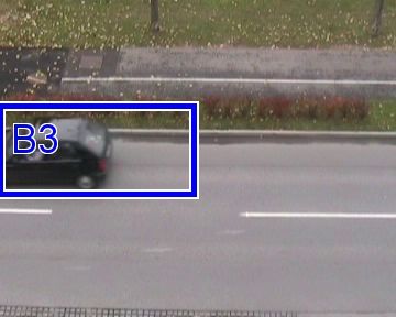
2

Experiments on climate data, videos, and text corpora will
demonstrate that our method can be applied to a variety of
applications without major adaptations.
     Despite the importance of this task across domains,
there has been very limited research on the detection of
anomalous intervals in multivariate time-series data, though       Figure 1. Schematic illustration of the principle of the MDI algorithm:
this problem has been known for a couple of years: Keogh et        The distribution of the data in the inner interval I is compared with the
al. [6] have already tackled this task in 2005 with a method       distribution of the remaining time-series in the outer interval Ω.
they called “HOT SAX”. They try to find anomalous sub-
sequences (“discords”) of time-series by representing all
possible sub-sequences of length d as a d-dimensional vector       2     M AXIMALLY D IVERGENT I NTERVALS
and using the Euclidean distance to the nearest neighbor in        This section formally introduces our MDI algorithm for off-
that space as anomaly score. More recently, Ren et al. [7]         line detection of anomalous intervals in spatio-temporal
use hand-crafted interval features based on the frequency of       data. After a set of definitions that we are going to make
extreme values and search for intervals whose features are         use of, we start by giving a very rough overview of the basic
maximally different from all other intervals. However, both        idea behind the algorithm, which is also illustrated schemat-
methods are limited to univariate data and a fixed length of       ically in Figure 1. The subsequent sub-sections will go into
the intervals must be specified in advance.                        more detail on the individual aspects and components of
     The latter is also true for a multivariate approach pro-      our approach.
posed by Liu et al. [8] who compare two consecutive in-                Our implementation of the MDI algorithm is available
tervals of fixed size in a time-series using the Kullback-         as open source at: https://cvjena.github.io/libmaxdiv/
Leibler or the Pearson divergence for detecting change-point
anomalies, i.e., points where a permanent change of the            2.1    Definitions
distribution of the data occurs. This is a different task than     Let X ∈ RT ×X×Y ×Z×D be a multivariate spatio-temporal
finding intervals that are anomalous with regard to all the        time-series given as 5th -order tensor with 4 contextual at-
remaining data. In addition, their method does not scale           tributes (point of time and spatial location) and D behav-
well for detecting anomalous intervals of dynamic size and is      ioral attributes for all N := T ·X·Y ·Z samples. We will index
hence not applicable for detecting other types of anomalies,       individual samples using 4-tuples i ∈ N4 like in Xi ∈ RD .
for which a broader context has to be taken into account.              The usual interval notation [`, r) will be used in the
     The task of detecting anomalous intervals of dynamic          following for discrete intervals {t ∈ N|` ≤ t < r}. Further-
size has recently been tackled by Senin et al. [9], who            more, the set of all intervals with size between a and b along
search for typical and anomalous patterns in time-series by        an axis of size n is denoted by
inducing a grammar on a symbolic discretization of the data.
As opposed to our approach, their method cannot handle                 In
                                                                        a,b := {[`, r) | 1 ≤ ` < r ≤ n + 1 ∧ a ≤ r − ` ≤ b} .            (1)
multivariate or spatio-temporal data.                                   The set of all sub-blocks of a data tensor X comply-
     Similar to our approach, Jiang et al. [10] search             ing with given size constraints A = (at , ax , ay , az ), B =
for anomalous blocks in higher-order tensors using the             (bt , bx , by , bz ) can then be defined as
Kullback-Leibler divergence, but apply their method to
discrete data only (e.g., relations in social networks) and         IA,B := {It × Ix × Iy × Iz |It ∈ ITat ,bt ∧ Ix ∈ IX
                                                                                                                      ax ,bx ∧
                                                                                                                                         (2)
use a Poisson distribution for modeling the data. Since                                               Iy ∈ IYay ,by ∧ Iz ∈ IZ
                                                                                                                            az ,bz } .
their search strategy is very specific to applications dealing
with graph data, it is not applicable in the general case for      In the following, we will often omit the indices for simplicity
multivariate continuous data dealt with in our work.               and just refer to it as I.
                                                                       Given any sub-block I ∈ IA,B , the remaining part of the
     Regarding spatio-temporal data, Wu et al. [11] follow a
                                                                   time-series excluding that specific range can be defined as
sequential approach for detecting anomalies first spatially,
then temporally and apply a merge-strategy afterwards.                      Ω(I) := ([1, T ] × [1, X] × [1, Y ] × [1, Z]) \ I            (3)
However, the time needed for merging grows exponentially
                                                                   and we will often simply refer to it as Ω if the corresponding
with the length of the time-series and their divergence
                                                                   range I is obvious from the context.
measure is limited to binary-valued data. In contrast to this,
our approach is able to deal with multivariate real-valued
data efficiently and treats time and space jointly.                2.2    Idea and Algorithm Overview
     The remainder of this article is organized as follows: Sec-   The approach pursued by the MDI algorithm to compute
tion 2 will introduce our novel “Maximally Divergent Inter-        anomaly scores for all intervals I ∈ I can be motivated by
vals” algorithm for off-line detection of collective anomalies     a long-standing definition of anomalies given by Douglas
in multivariate spatio-temporal data. Its performance will         Hawkins [12] in 1980, who defines an anomaly as “an
be evaluated quantitatively on artificial data in Section 3 and    observation which deviates so much from other observa-
its suitability for practical applications will be demonstrated    tions as to arouse suspicions that it was generated by a
by means of experiments on real data from various different        different mechanism”. In analogy to this definition, the MDI
domains in Section 4. Section 5 will summarize the progress        algorithm assumes that there is a sub-block I ∈ I of the
made so far and mention directions for future research.            given time-series that has been generated according to “a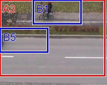
3

different mechanism” than the rest of the time-series in Ω (cf.     be updated efficiently is crucial. One such model is Kernel
the schematic illustration in Figure 1). The algorithm tries        Density Estimation (KDE) with
to capture these mechanisms by modelling the probability                               1 X
density pI of the data in the inner interval I and the distribu-           pS (Xi ) =         k(Xi , Xj ),   S ∈ {I, Ω} ,   (5)
                                                                                      |S| j∈S
tion pΩ in the outer interval Ω. We investigate two different
models for these distributions: Kernel Density Estimation           using a Gaussian kernel
(KDE) and multivariate normal distributions (Gaussians),                                                                       !
                                                                                                                           2
which will be explained in detail in Section 2.3.                                               D
                                                                                              2 −2             kx − yk
                                                                            k(x, y) = 2πσ              · exp −                     .   (6)
    Moreover, a measure D(pI , pΩ ) for the degree of “devia-                                                    2σ 2
tion” of pI from pΩ has to be defined. Like some other works
on collective anomaly detection [8], [10], we use—among             On the one hand, KDE is a very flexible model, but on
others—the Kullback-Leiber (KL) divergence for this purpose.        the other hand, it does not scale well to long time-series
However, Section 2.5 will show that this is a sub-optimal           and does not take correlations between attributes into ac-
choice when used without a slight modification and discuss          count. The second proposed model does not expose these
alternative divergence measures.                                    problems: It assumes that both the data in the anomalous
    Given these ingredients, the underlying optimization            interval I and in the remaining time-series Ω are distributed
problem for finding the most anomalous interval can be              according to multivariate normal distributions (Gaussians)
described as                                                        N (µI , SI ) and N (µΩ , SΩ ), respectively.

                 Iˆ = argmax D pI , pΩ(I) .                         2.3.2 Efficient Estimation with Cumulative Sums

                                                              (4)
                      I∈IA,B
                                                                    Both distribution models described above involve a sum-
     Various possible choices for the divergence measure D          mation over all samples in the respective interval. Perform-
will be discussed in Section 2.5.                                   ing this summation for multiple intervals is redundant,
     In order to actually locate this “maximally divergent          because some of them overlap with each other. Such a
interval” Iˆ, the MDI algorithm scans over all intervals I ∈        naı̈ve approach of finding the maximally divergent inter-
IA,B , estimates the distributions pI and pΩ and computes           val has a time complexity of O  N 2 · L2 with KDE and
the divergence between them, which becomes the anomaly              O (N · L · (N + L)) ⊆ O N 2 · L with Gaussian distribu-
score of the interval I . The parameters A and B , which            tions. This is due to the number of O (N · L) intervals (with
define the minimum and the maximum size of the intervals            L = (bt −at +1)·(bx −ax +1)·(by −ay +1)·(bz −az +1) being
in question, have to be specified by the user in advance.           the maximum volume of an interval), each of them requiring
This is not a severe restriction, since extreme values may          a summation over O (L) samples for the evaluation of one
be chosen for these parameters in exchange for increased            of the divergence measures described later in Section 2.5.
computation time. But depending on the application and the          For KDE, O(N ) distance computations are necessary for
focus of the analysis, there is often prior knowledge about         the evaluation of the probability density function for each
reasonable limits for the size of possible intervals.               sample, while for Gaussian distributions a summation over
                                                                    all O(N ) samples has to be performed for each interval to
     After the anomaly scores have been obtained for all inter-
                                                                    estimate the parameters of the distributions.
vals, they are sorted in descending order and non-maximum
                                                                        This would be clearly infeasible for large-scale data.
suppression is applied to obtain non-overlapping intervals
                                                                    However, these computations can be sped up significantly
only. For large time-series with more than 10k samples,
                                                                    by using cumulative sums [13]. For the sake of clarity, we
we apply an approximative non-maximum suppression that
                                                                    first consider the special case of a non-spatial time-series
avoids storing all interval scores by maintaining a fixed-size
                                                                    (xt )nt=1 , xt ∈ RD . With regard to KDE, a matrix C ∈ Rn×n
list of currently best-scoring non-overlapping intervals.
                                                                    of cumulative sums of kernelized distances can be used:
     Finally, the algorithm returns a ranking of intervals,
so that a user-specified number of top k intervals can be                                       t
                                                                                                X
                                                                                                   0

selected as output.                                                                   Ct,t0 =            k(xt , xt00 ) .               (7)
                                                                                                t00 =1

2.3     Probability Density Estimation                                  This matrix
                                                                                  has to be computed only once, which re-
                                                                    quires O n2 distance calculations, and can then be used to
The divergence measure used in (4) requires the notion of           estimate the probability density functions of the data in the
the distribution of the data in the intervals I and Ω. We will      intervals I = [a, b) and Ω = [1, n] \ I in constant time:
hence discuss in the following, which models we employ
to estimate these distributions and how this can be done
                                                                                             Ct,b−1 − Ct,a−1
efficiently.                                                                    pI (xt ) =                   ,
                                                                                                    |I|
                                                                                                                                       (8)
2.3.1    Models
                                                                                           Ct,n − Ct,b−1 + Ct,a−1
The choice of a specific model for the distributions pI and                     pΩ (xt ) =                        .
                                                                                                   n − |I|
pΩ imposes some assumptions about the data which may
not conform to reality. However, since the MDI algorithm               In analogy, a matrix C µ ∈ RD×n of cumulative sums
estimates the parameters of those distributions for all pos-        over the samples and a tensor C S ∈ RD×D×n of cumulative
sible intervals in the time-series, the use of models that can      sums over the outer products of the samples can be used
4

Figure 2. Illustration of time-delay embedding with κ = 3, τ = 4. The attribute vector of each sample is augmented with the attributes of the samples
4 and 8 time steps earlier.

to speed up the estimation of the parameters of Gaussian                    gap between two consecutive time-steps to be included as
distributions:                                                              context. An illustrative example is given in Figure 2.
                   t               t                                           This method is often motivated by Takens’ theorem [15],
            Ctµ =
                  X               X
                     xt0 , CtS =     xt0 · x>
                                            t0 ,      (9)                   which, roughly, states that for a certain embedding dimen-
                      t0 =1               t0 =1                             sion κ̄ the hidden state of the system can be reconstructed
where   Ctµ and    CtSare the t-th column of C µ and the t-th               given the observations of the last κ̄ time-steps.
                     S
D × D matrix of C , respectively. Using these matrices, the
                                                                            2.4.2 Spatial-Neighbor Embedding
mean vectors and covariance matrices can be estimated in
constant time.                                                              Correlations between nearby spatial locations are handled
    This technique can be generalized to the spatio-temporal                similarly: In addition to time-delay embedding, each sample
scenario using higher order tensors for storing the cumu-                   of a spatio-temporal time-series can be augmented by the
lative sums. The reconstruction of a sum over a given                       features of its spatial neighbors (cf. Figure 3) to enable
range from such a cumulative tensor follows the Inclusion-                  the detection of spatial or spatio-temporal anomalies. This
Exclusion Principle and the number of summands involved                     pre-processing step, which we refer to as spatial-neighbor
in the computation grows, thus, exponentially with the                      embedding, is parametrized with 3 parameters κx , κy , κz for
order of the tensor, being 16 for a 4th -order tensor, compared             the embedding dimension along each spatial axis and 3
to only 2 summands in the non-spatial case. The exact                       parameters τx , τy , τz for the lag along each axis.
equation describing the reconstruction in the general case                      Note that, in contrast to time-delay embedding, neigh-
of an M th -order tensor is given in Appendix A.                            bors from both directions are aggregated, since spatial con-
    Thanks to the use of cumulative sums, the compu-                        text is bilinear. For example, κx = 3 would mean to consider
tational complexity    of the MDI algorithm is reduced                      4 neighbors along the x-axis, 2 in each direction.
                                                            to                 Spatial-neighbor embedding can either be applied be-
O N 2 + N · L2 for the case of KDE and to O N · L2 for


Gaussian distributions.                                                     fore or after time-delay embedding. As opposed to many
                                                                            spatio-temporal anomaly detection approaches that perform
                                                                            temporal and spatial anomaly detection sequentially (e.g.,
2.4   Incorporation of Context
                                                                            [11], [16], [17]), the MDI algorithm in combination with the
The models used for probability density estimation de-                      two embeddings allows for a joint optimization. However, it
scribed in the previous section are based on the assump-                    implies a much more drastic multiplication of the data size.
tion of independent samples. However, this assumption is
almost never true for real data, since the value at a specific
                                                                            2.5   Divergences
point of time and spatial location is likely to be strongly
correlated with the values at previous times and nearby                     A suitable measure for the deviation of the distribution pI
locations. To mitigate this issue, we apply two kinds of                    from pΩ is an essential part of the MDI algorithm. The fol-
embeddings that incorporate context into each sample as                     lowing sub-sections introduce several divergence measures
pre-processing step.                                                        we have investigated and propose a modification to the
                                                                            well-known Kullback-Leibler (KL) divergence that is neces-
2.4.1 Time-Delay Embedding                                                  sary for being able to compare divergences of distributions
Aiming to make combinations of observed values more                         estimated from intervals of different size.
representative of the hidden state of the system being ob-
                                                                            2.5.1 Cross Entropy
served, time-delay embedding [14] incorporates context from
previous time-steps into each sample by transforming a                      Numerous divergence measures, including those described
                        n                                                   in the following, have been derived from the domain of
given time-series (xt )t=1 , xt ∈ RD , into another time-series
  0 n              0                                                        information theory. Being one of the most basic information
(xt )t=1+(κ−1)τ , xt ∈ RκD , given by
                                                                            theoretic concepts, the cross entropy between two distribu-
                                                  >
     x0t = x>     x>      x>      · · · x>             ,   (10)             tions given by their probability density functions p and q
             t      t−τ    t−2τ          t−(κ−1)·τ
                                                                            may already be used as a divergence measure:
where the embedding dimension κ specifies the number of
samples to stack together and the time lag τ specifies the                                DCE (p, q) := H(p, q) := Ep [− log q] .               (11)
5
κx = κy = 2, τx = τy = 1 κx = 3, κy = 2, τx = 3, τy = 2
Figure 3. Exemplary illustration of spatial-neighbor embedding with different parameters. The attribute vector of the sample with a solid fill color is
augmented with the attributes of the samples with a striped pattern.
Cross entropy measures how surprising a sample drawn is a known closed-form solution for the KL divergence of
from p is, assuming that it would have been drawn from q , two Gaussians [18]:
and is hence already eligible as a divergence measure, since
the unexpectedness grows when p and q are very different. 1 > −1
DKL (pI , pΩ ) = (µΩ − µI ) SΩ (µΩ − µI )
Since the MDI algorithm assumes, that the data in the 2
intervals I ∈ I and Ω have been sampled from the dis- |SΩ |
−1
tributions corresponding to pI and pΩ , respectively, the
+ trace SΩ SI + log − D . (15)
|SI |
cross entropy of the two distributions can be approximated
empirically from the data: This allows evaluating the KL divergence in constant
time for a given interval, which reduces the computational
1 X complexity of the MDI algorithm using the KL divergence
DCE (I, Ω) = log pΩ (Xi ) . (12) in combination with Gaussian models to the number of
g
|I| i∈I
possible intervals: O (N · L).
This approximation has the advantage of having to esti- Given this explicit solution for the KL divergence and
mate only one probability density, pΩ (xt ), explicitly. This is the closed-form solution for the entropy of a Gaussian
particularly beneficial, since the possibly anomalous inter- distribution [19] with mean vector µ and covariance matrix
vals I often contain only few samples, so that an accurate S , which is given by
estimation of the probability density pI is difficult. 1
H(N (µ, S)) = (log |S| + d + d · log (2π)) , (16)
2
2.5.2 Kullback-Leibler Divergence
one can easily derive a closed-form solution for the cross
The Kullback-Leibler (KL) divergence is a popular divergence entropy of those two distributions as well:
measure that builds upon the fundamental concept of cross
entropy. Given two distributions p and q , the KL divergence
H(pI , pΩ )
can be defined as follows:
= DKL (pI , pΩ ) + H(pI )
p
DKL (p, q) := H(p, q) − H(p, p) = Ep − log
. (13) 1 −1
q = trace SΩ SI + log |SΩ | + d · log(2π) (17)
2
As opposed to the pure cross entropy of p and q , the KL
−1
divergence does not only take into account how well p is ex- + (µΩ − µI )> SΩ (µΩ − µI ) .
plained by q , but also the intrinsic entropy H(p, p) =: H(p)
of p, so that an interval with a stable distribution would get Compared with the KL divergence, this does not assign
a higher score than an oscillating one if they had the same extremely high scores to small intervals I with a low vari-
cross entropy with the rest of the time-series. ance, due to the subtraction of log |SI |. This may be an
Like cross entropy, the KL divergence can be approxi- explanation for the evaluation results in Section 3, where
mated empirically from the data, but in contrast to cross cross entropy in combination with Gaussian models is often
entropy, this requires estimating the probability densities of superior to the KL divergence, although it does not account
both distributions, pI and pΩ : for intervals of varying entropy.
However, in contrast to the empirical approximation of
1 X pI (Xi ) cross entropy in (12), this requires the estimation of pI .
Dg KL (I, Ω) = · log
|I| i∈I pΩ (Xi )
(14) 2.5.3 Polarity of the KL divergence and its effect on MDI
1 X
= · log (pI (Xi )) − log (pΩ (Xi )) . It is worth noting that the KL divergence is not a metric and,
|I| i∈I
in particular, not symmetric: DKL (p, q) 6= DKL (q, p). Some
When used in combination with the Gaussian distribu- authors use, thus, a symmetric variant [8]:
tion model, the KL divergence comes with an additional 1 1
advantage from a computational point of view, since there DKL-SYM (p, q) = DKL (p, q) + DKL (q, p) . (18)
2 26
This raises the question whether DKL (pI , pΩ ), this bias is not related to the data itself, but to the length
DKL (pΩ , pI ), or the symmetric version DKL-SYM should be of the intervals: smaller intervals systematically get higher
used for the detection of anomalous intervals. Quantitative scores than longer ones. This harms the quality of interval
experiments with an early prototype of our method [20] detections, because anomalies will be split up into multiple
have shown that neither DKL (pΩ , pI ) nor DKL-SYM provide contiguous small detections (see Figure 5a for an example).
good performance, as opposed to DKL (pI , pΩ ). Recall that In m,m denotes the set of all intervals of length
A visual inspection of the detections resulting from m in a time-series with n time-steps. Furthermore, let ~0d , d ∈
the use of DKL (pΩ , pI ) with the assumption of Gaussian N, denote a d-dimensional vector with all coefficients being
distributions shows that all the intervals with the highest 0 and Id the identity matrix of dimensionality d.
anomaly scores have the minimum possible size specified When applying the MDI algorithm to a time-series
by the user and a very low variance. An example is given in (xt )nt=1 , xt ∼ N (~0d , Id ), sampled independently and iden-
Figure 4. The scores of the top detections in that example are tically from plain white noise, an ideal divergence is sup-
around 100 times higher than those yielded by DKL (pI , pΩ ). posed to yield constant average scores for all Im,m , m =
This bias of DKL (pΩ , pI ) towards small low-variance a, . . . , b (for some user-defined limits a, b), i.e., scores inde-
intervals can also be explained theoretically. For the sake pendent from the length of the intervals.
of simplicity, consider the special case of a univariate time- For simplicity, we will first analyze the distribution of
series. In this case, the closed-form solution for DKL (pΩ , pI ) those scores using the MDI algorithm with Gaussian dis-
assuming Gaussian distributions given in (15) reduces to tributions with the simple, but for this data perfectly valid
2
1 σΩ (µI − µΩ )2
assumption of identity covariance matrices. In this case, the
2 2
+ + log σI − log σΩ − 1 , (19) KL divergence DKL (pI , pΩ ) of two Gaussian distributions
2 σI2 σI2
with the mean vectors µI , µΩ ∈ Rd in some intervals
where µI , µΩ are the mean values and σI2 , σΩ 2
are the I ∈ Im , Ω = [1, n] \ I for some arbitrary m is given by
1 2
variances of the distributions in the inner and in the outer 2 kµΩ − µI k . Moreover, since all samples in the time-series
interval, respectively. It can be seen from (19) that, due to are normally distributed, so are their empirical means:
the division by σI2 , the KL divergence will approach infinity 1 X
when the variance in the inner interval converges towards µI = xt ∼ N (~0d , m−1 · Id ) ,
m t∈I
0. And since the algorithm has to estimate the variance
empirically from the given data, it assigns high detection
scores to intervals as small as possible, because smaller 1 X
intervals have a higher chance of having a low empirical µΩ = xt ∼ N (~0d , (n − m)−1 · Id ) .
n−m
t∈I
/
variance. The term log σI2 cannot counterbalance this effect,
though it is negative for σI < 1, since its absolute value Thus, all dimensions of the mean vectors are indepen-
grows much more slowly than that of σI−2 , as can be seen dent and identically normally distributed variables. Their
2 −2 −2
from the fact that ∀σ I7
(a) DKL (pI , pΩ ) (b) DU-KL (pI , pΩ )
Figure 5. (a) Top 10 detections obtained from the KL divergence on a real time-series and (b) top 3 detections obtained from the unbiased KL
divergence on the same time-series. This example illustrates the phenomenon of several contiguous minimum-size detections when using the
original KL divergence (note the thin lines between the single detections in the left plot). The MDI algorithm has been applied with a time-delay
embedding of κ = 3, τ = 1 and the size of the intervals to analyze has been limited to be between 25 and 250 samples.
µΩ , SΩ of the outer distribution converge towards the pa- from the use of the unbiased KL divergence compared with
rameters of the true distribution of the data. Thus, if the the original one can be seen in Figure 5.
restriction of the Gaussian model to identity covariance A further advantage of knowing the distribution of the
matrices is weakened to a global, shared covariance matrix scores is that this knowledge can also be used for normal-
S , the above findings also apply to the case of long time- izing the scores with respect to the number of attributes,
series with correlated variables and, hence, also when time- in order to make them comparable across time-series of
delay embedding is applied. Because in this case, the KL varying dimensionality. Moreover, it allows the selection
divergence reduces to 12 (µI − µΩ )> S −1 (µI − µΩ ) and the of a threshold for distinguishing between anomalous and
subtraction of the true mean µΩ followed by the multiplica- nominal intervals based on a chosen significance level. This
tion with the inverse covariance matrix can be considered may be preferred in some applications over searching for a
as a normalization of the time-series, transforming it to fixed number of top k detections.
standard normal variables with uncorrelated dimensions. Interestingly, Jiang et al. [10] have derived an equivalent
For the general case of two unrestricted Gaussian distri- unbiased KL divergence (m · DKL (pI , pΩ )) from a different
butions, the test statistic starting point based on the assumption of a Poisson dis-
tribution and the inverse log-likelihood of the interval as
−1
λ := dm(log(m) − 1) + m(µI − µΩ )> SΩ (µI − µΩ ) anomaly score.
−1 −1
+ trace mSI SΩ − m · log mSI SΩ (21)
2.5.5 Jensen-Shannon Divergence
has been shown to be asymptotically distributed according
d(d+1) A divergence measure that does not expose the problem
to a chi-squared distribution with d + degrees of
2 of being asymmetric is the Jensen-Shannon (JS) divergence,
freedom [21]. This test statistic is often used for testing
which builds upon the KL divergence:
the hypothesis that a given set of samples has been drawn
from a Gaussian distribution with known parameters [22]. 1 p+q 1 p+q
DJS (p, q) = DKL p, + DKL q, . (23)
In the scenario of the MDI algorithm, the set of samples 2 2 2 2
is the data in the inner interval I and the parameters of
the distribution to test that data against are those estimated where p and q are probability density functions. p+q 2 is a
from the data in the outer interval Ω. The null hypothesis mixture distribution, so that a sample is drawn either from
of the test would be that the data in I has been sampled p or from q with equal probability (though a parametrized
from the same distribution as the data in Ω. The test statistic version of the JS divergence accounting for unequal prior
may then be used as a measure for how well the data in the probabilities exists as well, but will not be covered here).
interval I fit the model established based on the data in the The JS divergence possesses some desirable properties,
remainder of the time-series. which the KL divergence does not have: most notably, it is
After some elementary reformulations, the relationship symmetric and bounded between 0 and log 2 [23], so that
between this test statistic λ and the KL divergence becomes anomaly scores cannot get infinitely high.
obvious: λ = 2m · DKL (pI , pΩ ). This is exactly the normal- Like the KL divergence, the JS divergence can be ap-
ization of the KL divergence by the scale factor identified in proximated empirically from the data in the intervals I
(20). Thus, we define an unbiased KL divergence as follows: and Ω. However, there is no closed-form solution for the
JS divergence under the assumption of a Gaussian dis-
DU-KL (pI , pΩ ) := 2 · |I| · DKL (pI , pΩ ) . (22) tribution (as opposed to the KL divergence), since pI +p 2
Ω
would then be a Gaussian Mixture Model (GMM). Though
The distribution of this divergence applied to asymp- several approximations of the KL divergence of GMMs have
totically long time-series depends only on the number d of been proposed, they are either computationally expensive
attributes and not on the length m of the interval any more. or abandon essential properties such as positivity [24]. This
However, this correction may also be useful for time-series lack of a closed-form solution is likely to be the reason
of finite length. An example of actual detections resulting why the JS divergence was clearly outperformed by the8
(a) amplitude change multvar (b) frequency change multvar
Figure 6. Two exemplary synthetic time-series along with the corresponding Hotelling’s T 2 scores and their gradients. The dashed black line
indicates the mean of the scores and the dashed blue line marks a threshold that is 1.5 standard deviations above the mean. Time-delay embedding
with κ = 3, τ = 1 was applied before computing the scores.
KL divergence in our quantitative experiments in Section 3 whose first and last samples are among these points if the
when the Gaussian model is used, despite its desirable interval conforms to the size constraints.
theoretic properties. This way, the probability density estimation and the
computation of the divergence have to be performed for
a comparatively small set of interesting intervals only and
2.6 Interval Proposals for Large-Scale Data not for all possible intervals in the time-series. The interval
Exploiting cumulative sums and a closed-form solution for proposal method is not required to have a low false-positive
the KL divergence, the asymptotic time complexity of the rate, though, because the divergence measure is responsible
MDI algorithm with a Gaussian distribution model could for the actual scoring. Instead, it has to act as a high-recall
already be reduced to be linear in the number of intervals system so that truly anomalous intervals are not excluded
(see Section 2.3.2). If the maximum length of an anomalous from the actual analysis.
interval is independent from the number of samples N , the Since we are only interested in the beginning and end of
run-time is also linear in N . However, due to high constant- the anomalies, the point-wise scores are not used directly,
time requirements for estimating probability densities and but the centralized gradient filter [−1 0 1] is applied to
computing the divergence, the algorithm is still too slow for the scores for reducing them in areas of constant anoma-
processing large-scale data sets with millions of samples. lousness and emphasizing changes of the anomaly scores.
Since anomalies are rare by definition, many of the The evaluation in Section 3.3 will show that the interval
intervals analyzed by a full scan will be uninteresting and proposal technique can speed-up the MDI algorithm signif-
irrelevant for the list of the top anomalies detected by the icantly without impairing its performance.
algorithm. In order to focus on the analysis of non-trivial in-
tervals, we employ a simple proposal technique that selects 3 E XPERIMENTAL E VALUATION
interesting intervals based on point-wise anomaly scores.
In this section, we evaluate our MDI algorithm on a quanti-
Simply grouping contiguous detections of point-wise
tative basis using synthetic data and compare it with other
anomaly detection methods in order to retrieve anomalous
approaches well-known in the field of anomaly detection.
intervals is insufficient, because it will most likely lead
to split-up detections. However, it is not unreasonable to
assume that many samples inside of an anomalous in- 3.1 Data Set
terval will also have a high point-wise score, especially In contrast to many other established machine learning
after applying contextual embedding. Figure 6, for example, tasks, there is no widely used standard benchmark for
shows two exemplary time-series from the synthetic data set the evaluation of anomaly detection algorithms; not for
introduced in Section 3.1 along with the point-wise scores the detection of anomalous intervals and not even for the
retrieved by applying the Hotelling’s T 2 method [4], after very common task of point-wise anomaly detection. This is
time-delay embedding has been applied to the time-series. mainly for the reason that the notion of an “anomaly” is
Note that even in the case of the very subtle amplitude- not well defined and varies between different applications
change anomaly, the two highest Hotelling’s T 2 scores are and even from analyst to analyst. Moreover, anomalies are,
at the beginning and the end of the anomaly. The idea is by definition, rare, which makes the collection of large-
to apply a simple threshold operation on the point-wise scale data sets difficult. However, even if a large amount
scores to extract interesting points and then propose all of data were available, it would be nearly impossible to
those intervals for detailed scoring by a divergence measure annotate it in an intersubjective way everyone would agree9
with. But accurate and complete ground-truth information
is mandatory for a quantitative evaluation and comparison
of machine learning techniques. Therefore, we use a syn-
thetic data set for assessing the performance of different
variants of the MDI algorithm.
All time-series in that data set have been
sampled from a Gaussian process GP(m, K)
with a squared-exponential covariance function
kxt −xt0 k2
−1/2
K(xt , xt0 ) = 2π` 2
· exp − 2`2 + σ · δ(t, t0 )
2
and zero mean function m(x) = 0. The length scale of the
GP has been set to `2 = 0.01 and the noise parameter to
σ 2 = 0.001. δ(t, t0 ) denotes Kronecker’s delta. Different
types of anomalies have then been injected into these
time-series, with a size varying between 5% and 20% of the
length of the time-series:
meanshift: A random, but constant value γ ∈ [3, 4] is added Figure 7. Examples from the synthetic test data set.
to or subtracted from the anomalous samples.
meanshift hard: A random, but constant value γ ∈ [0.5, 1]
3.2 Performance Comparison
is added to or subtracted from the anomalous samples.
meanshift5: Five meanshift anomalies are inserted into Since the detection of anomalous regions in spatio-temporal
the time-series. data is rather a detection than a classification task, we do not
use the Area under the ROC Curve (AUC) as performance
meanshift5 hard: Five meanshift_hard anomalies in-
criterion like many works on point-wise anomaly detection
serted into the time-series.
do, but quantify the performance in terms of Average Pre-
amplitude change: The time-series is multiplied with a cision (AP) with an Intersection over Union (IoU) criterion
Gaussian window with standard deviation L/4 whose mean that allows an overlap between 50% and 100%.
is the centre of the anomalous interval. Here, L is the length Hotelling’s T 2 [4] and Robust Kernel Density Estimation
of the anomalous interval and the amplitude of the Gaussian (RKDE) [3] are used as baselines for the comparison. For
window is clipped at 2.0. This modified time-series is added RKDE, a Gaussian kernel with a standard deviation of 1.0
to the original one. and the Hampel loss function are used. We obtain interval
frequency change: The time-series is sampled from a non- detections from those point-wise baselines by grouping
stationary GP, whose covariance function K(xt , xt0 ) = contiguous detections based on multiple thresholds and ap-
1/4 `2 (t)+`2 (t0 ) −1/2 2
plying non-maximum suppression afterwards. The overlap
`2 (t) · `2 (t0 ) · 2 · exp − `kx t −xt0 k
2 (t)+`2 (t0 ) +
0 2 threshold for non-maximum suppression is set to 0 in all
· −2
σ δ(t, t ) uses a reduced length scale ` (t) =
experiments to obtain non-overlapping intervals only. To
10 if t ∈/ [a, b),
during the anomalous interval I = be fair, MDI also has to compete with the baselines on the
10−4 if t ∈ [a, b)
task they have been designed for, i.e., point-wise anomaly
[a, b), so that correlations between samples are reduced,
detection, by means of AUC. The interval detections can be
which leads to more frequent oscillations [25].
converted to point-wise detections easily by taking the score
mixed: The values in the anomalous interval are replaced of the interval a sample belongs to as score for that sample.
with the values of another function sampled from the Figure 8 shows that the performance of the MDI al-
Gaussian process. 10 time-steps at the borders of the gorithm using the Gaussian model is clearly superior on
anomaly are interpolated between the two functions for a the entire synthetic data set compared to the baselines by
smooth transition. This rather difficult test case is supposed means of Mean AP and even on the task of point-wise
to reflect the concept of anomalies as being “generated by a anomaly detection measured by AUC. The DKL (pI , pΩ ) po-
different mechanism” (cf. Section 2.2). larity of the KL divergence has been used in all experiments
following the argumentation in Section 2.5.3. In addition,
The above test cases are all univariate, but the performance of the unbiased variant DU-KL (pI , pΩ ) is
there are as well similar multivariate scenarios reported for the Gaussian model. The parameters of time-
meanshift_multvar, amplitude_change_multvar, delay embedding have been fixed to κ = 6, τ = 2 which we
frequency_change_multvar, and mixed_multvar have empirically found to be suitable for this data set. For
with 5-dimensional time-series. Regarding the first three KDE, we used a Gaussian kernel with bandwidth 1.0.
of these test cases, the corresponding anomaly is injected While MDI KDE is already superior to the baselines,
into one of the dimensions, while all attributes are replaced it is significantly outperformed by MDI Gaussian, which
with those of the other time-series in the mixed_multvar improves on the best baseline by 286%. This discrepancy
scenario, which is also a property of many real time-series. between the MDI algorithm using KDE and using Gaussian
This results in a synthetic test data set with 11 test cases, models is mainly due to time-delay embedding, which is
a total of 1100 time-series and an overall number of 1900 particularly useful for the Gaussian model, because it takes
anomalies. Examples for all test cases are shown in Figure 7. correlations of the variables into account, as opposed to10
Figure 8. Performance comparison of different variants of the MDI algorithm and the baselines on the synthetic data set.
Figure 9. Effect of time-delay embedding with κ = 6, τ = 2 on the performance Figure 10. Performance of the original and the unbiased KL
of the MDI algorithm and the baselines on the synthetic data set. divergence on test cases with multiple or subtle anomalies.
KDE. As can be seen in Figure 9, the Gaussian model would 3.3 Interval Proposals
be worse than KDE and on par with the baselines without In order not to sacrifice detection performance for the sake
time-delay embedding. of speed, the interval proposal method described in Sec-
Considering the Mean AP on this synthetic data set, tion 2.6 has to act as a high-recall system proposing the
the unbiased KL divergence did not perform better than majority of anomalous intervals. This can be controlled to
the original KL divergence. However, on the test cases some degree by adjusting the threshold θ = µ+ϑ·σ applied
meanshift5, meanshift5_hard, and meanshift_hard to the point-wise scores, where µ and σ are the empirical
it achieved an AP twice as high as that of DKL (pI , pΩ ), which mean and standard deviation of the point-wise scores, re-
was poor on those data sets (see Figure 10). Since real data spectively. To find a suitable value for the hyper-parameter
sets are also likely to contain multiple anomalies, we expect ϑ, we have evaluated the recall of the proposed intervals for
DU-KL to be a more reliable divergence measure in practice. different values of ϑ ∈ [0, 4] using the usual IoU measure for
Another interesting result is that cross entropy was the distinguishing between true and false positive detections.
best performing divergence measure. This shows the ad- The results in Figure 11a show that time-delay embedding is
vantage of reducing the impact of the inner distribution pI , of a great benefit in this scenario too. Based on these results,
which is estimated from very few samples. However, it may we selected ϑ = 1.5 for subsequent experiments, which still
perform less reliably on real data whose entropy varies more provides a recall of 97% and is already able to reduce the
widely over time than in this synthetic benchmark. number of intervals to be analyzed in detail significantly.
The processing of all the 1100 time-series from the syn-
The Jensen-Shannon divergence performed best for the thetic data set, which took 216 seconds on an Intel Core™
KDE method, but worst for the Gaussian model. This can i7-3930K with 3.20GHz and eight virtual cores using the
be explained by the lack of a closed-form solution for the Gaussian model and the unbiased KL divergence after the
JS divergence, so that it has to be approximated from the usual time-delay embedding with κ = 6, τ = 2, could
data, while the KL divergence of two Gaussians can be be reduced to 5.2 seconds using interval proposals. This
computed exactly. This advantage of the combination of corresponds to a speed-up by more than 40 times.
the KL divergence with Gaussians models is, thus, not only Though impressive, the speed-up was expected. What
beneficial with respect to the run-time of the algorithm, but was not expected, however, is that the use of interval pro-
also with respect to its detection performance. posals also increased the detection performance of the entire
The differences between the results in Figure 8 are sig- algorithm by up to 125%, depending on the divergence. The
nificant on a level of 5% according to the permutation test. exact average precision achieved by the algorithm on the11
(a) Proposal Recall (b) Effect of Interval Proposals
Figure 11. (a) Recall of interval proposals without time-delay embedding and with κ = 6, τ = 2 on the synthetic data set for different proposal
thresholds. (b) Effect of interval proposals on the Mean Average Precision of different variants of the MDI algorithm on the synthetic data set.
synthetic data set with a full scan over all intervals and the so-called “Hamburg-Flut” which flooded one fifth of
with interval proposals is shown in Figure 11b. This im- Hamburg in February 1962 and caused 340 deaths. Also
provement is also reflected by the AUC scores not reported among the top 5 is the “North Frisian Flood”, which was
here and is, hence, not specific to the evaluation criterion. a severe surge in November 1981 and lead to several dike
A possible explanation for this phenomenon is that some breaches in Denmark.
intervals that are uninteresting but distracting for the MDI A visual inspection of the remaining 22 detections re-
algorithm are not even proposed for detailed analysis. vealed, that almost all of them are North Sea storms as well.
Only 4 of them are not storms, but the opposite: they span
4 A PPLICATION E XAMPLES ON R EAL DATA times of extremely calm sea conditions with nearly no wind
and very low waves, which is some kind of anomaly as well.
The following application examples on real data from var-
A list of the top 50 detections can be found in
ious different domains are intended to complement the
Appendix B and animated heatmaps of the three vari-
quantitative results presented above with a demonstration
ables during the detected time-frames are shown on
of the feasibility of our approach for real problems.
our web page: http://www.inf-cv.uni-jena.de/libmaxdiv
applications.html.
4.1 Detection of North Sea Storms Processing this comparatively long time-series using 8
To demonstrate the efficiency of the MDI algorithm on long parallel threads took 27 seconds. This time can be reduced
time-series, we apply it to storm detection in climate data: further to half a second by using interval proposals without
The coastDat-1 hindcast [26] is a reconstruction of various changing the top 10 detections significantly. This supports
marine climate variables measured at several locations over the assumption, that the novel proposal method does not
the southern North Sea between 51° N, 3° W and 56° N, only perform well on synthetic, but also on real data.
10.5° E with an hourly resolution over the 50 years from
1958 to 2007, i.e., approximately 450,000 time steps. Since
4.2 Spatio-Temporal Detection of Low Pressure Areas
measurements are not available at locations over land, we
select the subset of the data between 53.9° N, 0° E and 56° As a genuine spatio-temporal use-case, we have also applied
N, 7.7° E, which results in a regular spatial grid of size the MDI algorithm to a time-series with daily sea-level
78 × 43 located entirely over the sea (cf. Figure 12). Because pressure (SLP) measurements over the North Atlantic Sea
cyclones and other storms usually have a large spatial extent with a much wider spatial coverage than in the previous
and move over the region covered by the measurements, experiment. For this purpose, we selected a subset of the
we reduce the spatio-temporal data to purely temporal data NCEP/NCAR reanalysis [27] covering the years from 1957
in this experiment by averaging over all spatial locations. to 2011. This results in a time-series of about 20,000 days.
The variables used for this experiment are significant wave The spatial resolution of 2.5° degrees is rather coarse and
height, mean wave period and wind speed. the locations are organized in a regular grid of size 28 × 17
We apply the MDI algorithm to that data set using the covering the area between 25° N, 52.5° W and 65° N, 15° E.
Gaussian model and the unbiased KL divergence. Since Again, the MDI algorithm with the Gaussian model
North Sea storms lasting longer than 3 days are usually and the unbiased KL divergence is applied to this time-
considered two independent storms, the maximum length series to detect low-pressure fields, which are related to
of the possible intervals is set to 72 hours, while the mini- storms. Regarding the time dimension, we apply time-delay
mum length is set to 12 hours. The parameters of time-delay embedding with κ = 3, τ = 1 and search for intervals of
embedding are fixed to κ = 3, τ = 1. size between 3 and 10 days. Concerning space, we do not
28 out of the top 50 and 7 out of the top 10 detections apply any embedding for now and set a minimum size of
returned by the algorithm can be associated with well- 7.5° × 7.5°, but no maximum. 7 out of the top 20 detections
known historic storms. The highest scoring detection is could be associated with known historic storms.12
The MDI algorithm using the unbiased KL divergence is
then applied in order to search for anomalous sequences
of between 10 and 50 sentences in the mixed-language
text after sentence-wise transformation to the feature space.
Because the number of features is quite high in relation
to the number of samples in an interval, we use a global
covariance matrix shared among the Gaussian models and
do not apply time-delay embedding.
The top 5 detections returned by the algorithm corre-
Figure 12. Map of the area covered by the coastDat dataset. The spond to the 5 German paragraphs that have been injected
highlighted box denotes the area from which data have been aggregated into the English text. The localization is quite accurate,
for our experiment. though not perfect: on average, the boundaries of the de-
tected paragraphs are off by 1.4 sentences from the ground-
truth. The next 5 detections are mainly tables and enumer-
A visual inspection of the results shows that the MDI
ations, which are also an anomaly compared with the usual
algorithm is not only capable of detecting occurrences of
dialog style of the parliament proceedings.
anomalous low-pressure fields over time, but also their
For this scenario, we had designed the features specifi-
spatial location. This can be seen in the animations on
cally for the task of language identification. To see what else
our web page: http://www.inf-cv.uni-jena.de/libmaxdiv
would be possible with a smaller bias towards a specific
applications.html. A few snapshots and a list of detections
application, we have also applied the algorithm to the 1st
are also shown in Appendix C.
Book of Moses (Genesis) in the King James Version of the
It is not necessary to apply spatial-neighbor embedding
bible, where we use word2vec [29] for word-wise feature
in this scenario, since we are not interested in spatial out-
embeddings. word2vec learns real-valued vector represen-
liers, but only in the location of temporal outliers. We have
tations of words in a way, so that the representations of
also experimented with applying spatial-neighbor embed-
words that occur more often in similar contexts have a
ding and it led to the detection of some high-pressure fields
smaller Euclidean distance. The embeddings used for this
surrounded by low-pressure fields. Since high-pressure
experiment have been learned from the Brown corpus using
fields are both larger and more common in this time-series,
the continuous skip-gram model and we have chosen a di-
they are not detected as temporal anomalies.
mensionality of 50 for the vector space, which is rather low
Since we did not set a maximum spatial extent of
for word2vec models, but still tractable for the Gaussian
anomalous regions, the algorithm took 4 hours to process
probability density model. Words which have not been seen
this spatio-temporal time-series. This could, however, be re-
by the model during training are treated as missing values.
duced to 22 seconds using our interval proposal technique,
with only a minor loss of localization accuracy. The top 10 detections of sequences of between 50 and
500 words according to the unbiased KL divergence are
provided in Appendix D. The first five of those are, without
4.3 Stylistic Anomalies in Texts of Natural Language exception, genealogies, which can indeed be considered as
By employing a transformation from the domain of natural anomalies, because they are long lists of names of fathers,
language to real-valued features, the MDI algorithm can sons and wives, connected by repeating phrases. The 6th
also be applied to written texts. One important task in detection is a dialog between God and Abraham, where
Natural Language Processing (NLP) is, for example, the Abraham bargains with God and tries to convince him not
identification of paragraphs written in a different language to destroy the town Sodom. This episode is another example
than the remainder of the document. Such a segmentation for stylistic anomalies, since the dialog is a concatenation of
can be used as a pre-processing step for the actual, language- very similar question-answer pairs with only slight modifi-
specific processing. cations.
In order to simulate such a scenario, we use a subset of Due to the rather wide limits on the possible size of
the Europarl corpus [28], which is a sentence-aligned parallel anomalous intervals, the analysis of the entire book Genesis,
corpus extracted from the proceedings of the European a sequence of 44,764 words, took a total of 9 minutes, where
Parliament in 21 different languages. The 33,334 English we have not yet used interval proposals.
sentences from the COMTRANS subset of Europarl, which
is bundled with the Natural Language Toolkit (NLTK) for
Python, serve as a basis and 5 random sequences of between 4.4 Anomalies in Videos
10 and 50 sentences are replaced by their German counter- The detection of unusual events in videos is another impor-
parts to create a semantically coherent mixed-language text. tant task, e.g., in the domain of video surveillance or indus-
We employ a simple transformation of sentences to trial control systems. Though videos are already represented
feature vectors: Since the distribution of letter frequencies as multivariate spatio-temporal time-series with usually 3
varies across languages, each sentence is represented by a variables (RGB channels), a semantically more meaningful
27-dimensional vector whose first element is the average representation can be obtained by extracting features from a
word length in the sentence and the remaining 26 compo- Convolutional Neural Network (CNN).
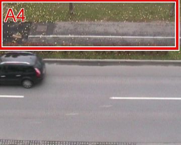
nents are the absolute frequencies of the letters “a” to “z” In this experiment, we use a video of a traffic scene from
(case-insensitive). German umlauts are ignored since they the ViSOR repository [30]. It has a length of 60 seconds (1495
would make the identification of German sentences too easy. frames) and a rather low resolution of 360 × 288 pixels.You can also read