Faster decline and higher variability in the sea ice thickness of the marginal Arctic seas when accounting for dynamic snow cover
←
→
Page content transcription
If your browser does not render page correctly, please read the page content below
The Cryosphere, 15, 2429–2450, 2021
https://doi.org/10.5194/tc-15-2429-2021
© Author(s) 2021. This work is distributed under
the Creative Commons Attribution 4.0 License.

Faster decline and higher variability in the sea ice thickness of the
marginal Arctic seas when accounting for dynamic snow cover
Robbie D. C. Mallett1 , Julienne C. Stroeve1,2,3 , Michel Tsamados1 , Jack C. Landy4,5 , Rosemary Willatt1 ,
Vishnu Nandan3 , and Glen E. Liston6
1 Centre for Polar Observation and Modelling, Earth Sciences, University College London, London, UK
2 National Snow and Ice Data Center, University of Colorado, Boulder, CO, USA
3 Centre for Earth Observation Science, University of Manitoba, Winnipeg, Canada
4 School of Geographical Sciences, University of Bristol, Bristol, UK
5 Department of Physics and Technology, UiT The Arctic University of Norway, Tromsø, Norway
6 Cooperative Institute for Research in the Atmosphere, Colorado State University, Fort Collins, CO, USA

Correspondence: Robbie D. C. Mallett (robbie.mallett.17@ucl.ac.uk)

Received: 25 September 2020 – Discussion started: 28 October 2020
Revised: 9 March 2021 – Accepted: 31 March 2021 – Published: 4 June 2021

Abstract. Mean sea ice thickness is a sensitive indicator of      1   Introduction
Arctic climate change and is in long-term decline despite sig-
nificant interannual variability. Current thickness estimations
from satellite radar altimeters employ a snow climatology         Sea ice cover moderates the exchange of moisture, heat and
for converting range measurements to sea ice thickness, but       momentum between the atmosphere and the polar oceans, in-
this introduces unrealistically low interannual variability and   fluencing regional ecosystems, hemispheric weather patterns
trends. When the sea ice thickness in the period 2002–2018        and global climate. Sea ice thickness (SIT) is a key charac-
is calculated using new snow data with more realistic vari-       teristic of the sea ice cover, as thicker sea ice weakens the
ability and trends, we find mean sea ice thickness in four of     coupling between the ocean and atmosphere systems.
the seven marginal seas to be declining between 60 %–100 %           Thicker sea ice is more thermally insulating and limits
faster than when calculated with the conventional climatol-       heat transfer from the ocean to the atmosphere in winter and
ogy. When analysed as an aggregate area, the mean sea ice         consequent thermodynamic growth (Petty et al., 2018a). SIT
thickness in the marginal seas is in statistically significant    also exerts control on sea ice dynamics and rheology (Tsama-
decline for 6 of 7 winter months. This is observed despite a      dos et al., 2013; Vella and Wettlaufer, 2008). The thickness
76 % increase in interannual variability between the methods      of sea ice during snow accumulation also dictates whether
in the same time period. On a seasonal timescale we find that     the sea ice surface drops below the waterline, potentially in-
snow data exert an increasingly strong control on thickness       creasing thermodynamic sea ice growth through the forma-
variability over the growth season, contributing 46 % in Oc-      tion of snow ice (Rösel et al., 2018). The impact of the end-
tober but 70 % by April. Higher variability and faster decline    of-winter SIT distribution persists into the melt season with
in the sea ice thickness of the marginal seas has wide impli-     thick sea ice decreasing the transmission of solar radiation
cations for our understanding of the polar climate system and     to the surface ocean and reducing the potential for in- and
our predictions for its change.                                   under-ice primary productivity (Mundy et al., 2005; Katlein
                                                                  et al., 2015). Finally, thick sea ice is far more likely to survive
                                                                  the melt season, increasing the average age of Arctic sea ice.
                                                                  Correct assimilation of ice thickness into models therefore
                                                                  offers opportunities for prediction of the sea ice state on sea-
                                                                  sonal timescales (Chevallier and Salas-Mélia, 2012; Block-
                                                                  ley and Peterson, 2018; Schröder et al., 2019).

Published by Copernicus Publications on behalf of the European Geosciences Union.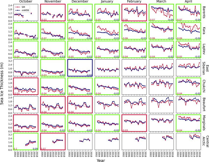
2430                                                      R. D. C. Mallett et al.: Snow’s impact on SIT variability and trends

   The annual sea ice thickness distribution is highly spatially    that sea ice is likely thinning at a faster rate in some marginal
variable, with a cover of thick multi-year ice in the Central       seas than previously thought, because the snow water equiv-
Arctic and a thinner, more seasonally variable cover of first-      alent on the sea ice is declining too.
year ice in the marginal seas. Regional sea ice thickness dis-
tributions are often characterised by the mean thickness, SIT.      The role of snow in radar-altimetry-derived sea ice
As well as being a key parameter for the processes described        thickness retrievals
above, the value can be multiplied by the sea ice area to pro-
duce the sea ice volume, one of the most sensitive indicators       Satellite radar altimetry involves the emission of radar
of Arctic climate change (Schweiger et al., 2019).                  pulses from a satellite and the subsequent detection of their
   While continuous and consistent monitoring of pan-Arctic         backscatter. The time difference between emission and detec-
SIT has not been achieved on a multi-decadal timescale, a           tion (time of flight) corresponds to the distance travelled and
combination of different techniques has suggested a signifi-        thus the height of the transmitter above the scattering surface.
cant decline in thickness since 1950 (Kwok, 2018; Stroeve           Radar altimeters of different frequencies have been carried
and Notz, 2018). Satellite altimeters using both radar and          on board several earth observation satellites such as ERS-1/2,
lidar have provided a valuable record of changing sea ice           Envisat, AltiKa, CryoSat-2 and Sentinel-3A/B (Quartly et al.,
thickness but have often been limited for various reasons.          2019). We now quantify the role of snow cover in conven-
Some have been limited spatially by their orbital inclination       tional sea ice thickness estimation, before revealing and ex-
(e.g. the European Remote Sensing (ERS) satellites, Envisat,        plaining the effects of previously unincorporated trends and
AltiKa and Sentinel radar altimeters have operated up to only       variability.
81.5◦ N) and others in temporal coverage (e.g. ICESat was              The Ku-band radar waves emitted from CryoSat-2 are gen-
operated in campaign mode rather than providing continu-            erally assumed in mainstream SIT products to scatter from
ous coverage). Two satellite altimeters currently offer contin-     the snow/sea ice interface (Kurtz et al., 2014; Tilling et al.,
uous and meaningfully pan-Arctic monitoring of the Arctic           2018; Hendricks and Ricker, 2019; Landy et al., 2020). The
sea ice: the ICESat-2 and CryoSat-2 altimeters. ICESat-2 has        difference in radar ranging (derived from time of flight) be-
been in operation since September 2018 and so far has doc-          tween areas of open water and areas of sea ice is known as the
umented only two winters of sea ice thickness (Kwok et al.,         radar freeboard, fr . The height of the sea ice surface above
2020).                                                              the waterline is referred to as the sea ice freeboard, fi . This
   Although the launch of the CryoSat-2 radar altimeter             is extracted from the radar freeboard through (a) assuming
(henceforth CS2) in 2010 allowed significant advances in            that the primary scattering horizon corresponds to the sea ice
understanding the spatial distribution and interannual vari-        surface and (b) accounting for the slower radar wave propa-
ability of pan-Arctic SIT (Laxon et al., 2013), a statistically     gation through the snow cover above the sea ice surface (Ar-
significant decreasing trend within the CS2 observational pe-       mitage and Ridout, 2015; Mallett et al., 2020). The sea ice
riod has not been detected for the Arctic as a whole. The           freeboard can then be converted to sea ice thickness by con-
lack of certainty regarding any trend in SIT is in part due to      sidering the floe’s hydrostatic equilibrium given the sea ice
the various uncertainties associated with SIT retrieval from        density and weight of overlying snow. In the simplified case
radar altimetry (Ricker et al., 2014; Zygmuntowska et al.,          of bare sea ice, we would calculate
2014). Major contributors to these uncertainties are the rela-                       ρw
                                                                    SITbare = fr           ,                                     (1)
tively large footprint of a radar pulse when compared to laser                     ρw − ρi
altimetry, the variable density of sea ice, retracking of radar
returns from rough sea ice, and the need for an a priori snow-      where ρw is the density of seawater and ρi the density of
depth and density distribution (Kern et al., 2015; Landy et al.,    sea ice. In order to adjust the above equation for the pres-
2020).                                                              ence of overlying snow, the twin effects of the snow’s weight
   The impact of snow-depth uncertainty on SIT retrievals           and the snow’s delaying influence on radar pulse propaga-
was recently included by the IPCC in a list of “Key Knowl-          tion must be taken into account. These three influences on
edge Gaps and Uncertainties” (Meredith et al., 2019). More          SIT (the radar freeboard measurement, the pulse propagation
specifically, Bunzel et al. (2018) found snow to have a strong      delay and the freeboard depression from snow weight) can
influence on the interannual variability of SIT and conse-          therefore be expressed as three terms (see Supplement) in
quent detection of thickness trends. Here we investigate the        the following way:
impact of a new, pan-Arctic snow-depth and density data                         ρw           ρw

                                                                                                     c

                                                                                                                      ρs
set (SnowModel-LG; Liston et al., 2020a; Stroeve et al.,            SIT = hr          + hs             − 1 + hs            . (2)
                                                                              ρw − ρi      ρw − ρi c s             ρw − ρi
2020) on trends and variability in regional SIT when used in
place of the traditional, climatological data set (Warren et al.,      In this paper we introduce a simple method for combin-
1999). We show that traditional calculations of SIT omit sig-       ing the second and third terms of the above equation into
nificant interannual variability due to their reliance on a snow    a single term that is proportional to the snow water equiva-
climatology, and we quantify this omission. We also show            lent (Sect. 3.1). This helps to easily separate the influences of

The Cryosphere, 15, 2429–2450, 2021                                                      https://doi.org/10.5194/tc-15-2429-2021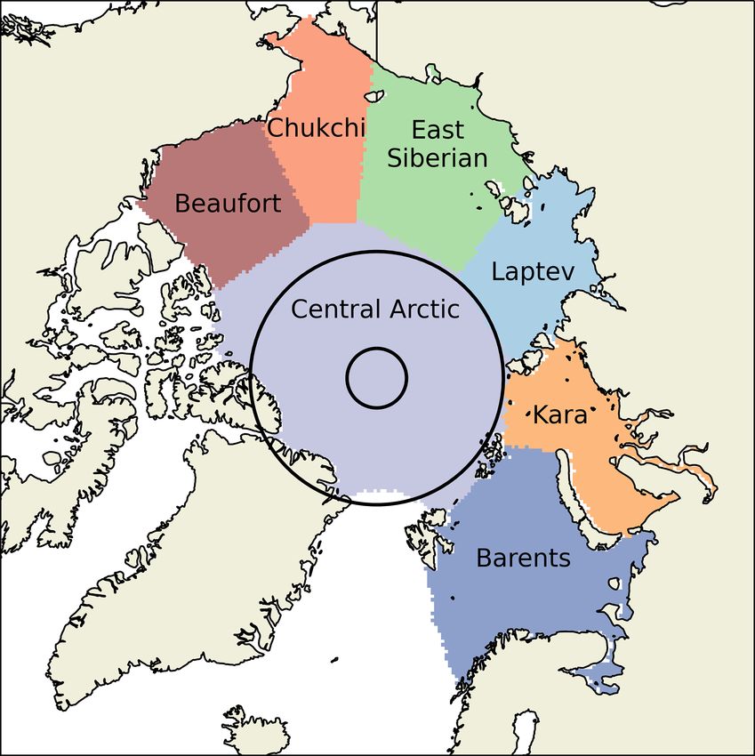
R. D. C. Mallett et al.: Snow’s impact on SIT variability and trends                                                              2431

                                                                       et al., 2018) and (b) it is publicly available for download.
                                                                       CS2 carries a delay-Doppler altimeter that significantly en-
                                                                       hances along-track resolution by creating a synthetic aper-
                                                                       ture. For this reason as well as its higher latitudinal limit, we
                                                                       used CS2 radar freeboard measurements over Envisat during
                                                                       the period when the missions overlapped (November 2010–
                                                                       March 2012). To create a radar freeboard product that is con-
                                                                       sistent between the Envisat and CS2 missions, Envisat re-
                                                                       turns are retracked using a variable threshold retracking algo-
                                                                       rithm. This variable threshold is calculated from the strength
                                                                       of the surface backscatter and the width of the leading edge of
                                                                       the return waveform such that the inter-mission bias is min-
                                                                       imised (Paul et al., 2018). The results are comprehensively
                                                                       analysed in the Product Validation & Intercomparison Re-
                                                                       port (Kern et al., 2018). One key finding of this report is
                                                                       that while Envisat radar freeboards are calculated so as to
                                                                       match CS2 freeboards during the period of overlap over the
                                                                       whole Arctic Basin, there are biases over ice types. In partic-
                                                                       ular, Envisat ice freeboards (not radar freeboards) are biased
                                                                       2–3 cm low (relative to CS2) in areas dominated by multi-
                                                                       year ice (MYI) and 2–3 cm high in areas dominated by first-
Figure 1. The definitions of the marginal Arctic seas used in this     year ice (FYI). We discuss the implications of these biases in
paper, from Stroeve et al. (2014). Two black, concentric circles in-
                                                                       Sect. 5.3.
dicate the latitudinal limits of the CryoSat-2 (inner circle; 88◦ N)
                                                                          While the ESA CCI data are only available from the CCI
and Envisat (outer circle; 82.5◦ N) missions.
                                                                       website until the winter of 2016/17, the CryoSat-2 radar free-
                                                                       boards in these data are identical to the CS2 radar free-
snow data and radar freeboard measurements on the determi-             board product of the Alfred Wegener Institute (Hendricks
nation of sea ice thickness. Specifically, we compare the im-          and Ricker, 2019, this was manually confirmed). We were
pact of two snow products on regional trends and variability           therefore able to extend our radar freeboard time series
in sea ice thickness. These products are the snow climatology          through the winter of 2017/18, which is when our snow data
given by Warren et al. (1999) and the output of SnowModel-             from SnowModel-LG (see below) ends.
LG (Liston et al., 2020a; Stroeve et al., 2020).                          All radar freeboard data used in this study are supplied on
                                                                       a 25 km EASE grid (Brodzik et al., 2012), the same as that
                                                                       of SnowModel-LG.
2     Data description
                                                                       2.3   The Warren climatology (W99)
2.1    Regional mask

We define seven regions of the Arctic Basin using the mask             The most commonly used radar-altimetry SIT products use
from Stroeve et al. (2014), which is gridded onto a 25 km              algorithms developed by the Centre for Polar Observation
resolution EASE grid (Brodzik et al., 2012, Fig. 1). We define         and Modelling, the Alfred Wegener Institute and the NASA
the “marginal seas” of the Arctic Basin as the colour-coded            Goddard Space Flight Center (Tilling et al., 2018; Hendricks
areas of Fig. 1 excluding the Central Arctic. All constituent          and Ricker, 2019; Kurtz et al., 2014). Another commonly
regions of the marginal seas grouping lie within the coverage          used but not publicly available product is from the NASA Jet
of Envisat barring a negligible portion of the Laptev Sea.             Propulsion Laboratory (Kwok and Cunningham, 2015). All
                                                                       four groups utilise modified forms of the snow climatology
2.2    Radar freeboard data                                            assembled by Warren et al. (1999) from the observations of
                                                                       Soviet drifting stations between 1954 and 1991 (henceforth
To examine the impact of snow products on Envisat/CryoSat-             referred to as W99).
2 thickness retrievals, we used radar freeboard data from the             While the consistent use of W99 for sea ice thickness cal-
ESA Sea Ice Climate Change Initiative (Hendricks et al.,               culation is convenient for intercomparison of products (e.g.
2018a). These data are available from October in the winter            Sallila et al., 2019; Landy et al., 2020), the data have a num-
of 2002/03 until April in the winter of 2016/17. This prod-            ber of drawbacks. This work is centred around two key issues
uct was chosen for two main reasons: (a) it provides a con-            with the use of W99 for SIT retrieval: inadequate representa-
sistent record for both the Envisat and CS2 missions (Paul             tion of interannual variability and trends.

https://doi.org/10.5194/tc-15-2429-2021                                                      The Cryosphere, 15, 2429–2450, 2021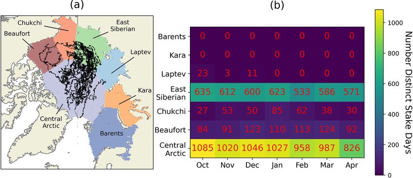
2432                                                     R. D. C. Mallett et al.: Snow’s impact on SIT variability and trends

   The Warren climatology includes quadratic fits for every        flights which showed reduced snow depth over first-year ice
month of snow water equivalent and snow depth. We pro-             (Kurtz and Farrell, 2011). This implementation, known as
jected these fits over the 361 × 361 EASE grid (for combi-         “mW99”, consists of halving snow depths over first-year ice
nation with our radar freeboard data and comparison with           with snow density kept constant. Because the areal fraction
SnowModel-LG) to create snow water equivalent (SWE)                and spatial distribution of FYI changes from year to year, this
and depth distributions across the Arctic Basin as defined in      modification introduces a small degree of interannual vari-
Sect. 2.1.                                                         ability into the contribution of snow data to sea ice thickness.
                                                                   We investigate this in Sect. 4.1.1.
Drifting station coverage illustration
                                                                   2.5   Ice type data
At this point it is instructive to briefly illustrate the cover-
age of the drifting stations from which W99 was compiled.          Sea ice type data are required to modify W99 and create
We analysed position and snow-depth data from the 28 drift-        mW99. One popular product for this (e.g. Tilling et al., 2018;
ing stations that contributed to W99 (Fig. 2a). It is clear        Hendricks and Ricker, 2019) is an operational product from
that the vast majority of these operated in the Central Arctic     the EUMETSAT Ocean and Sea Ice Satellite Application Fa-
or in the East Siberian Sea, with very little sampling done        cility (OSI SAF, http://www.osi-saf.org/, last access: 10 May
in most other marginal seas. But while these tracks illus-         2021). However, this data series begins in March 2005. This
trate the movements of the drifting stations, it is important      is after our study begins (in October 2002).
to note that the stations were not always collecting snow             A similar product exists, published by the Copernicus
data which would contribute to the W99 climatology. To             Climate Data Store (CDS, https://cds.climate.copernicus.eu/,
assess the spatial distribution of snow sampling, we cross-        last access: 10 April 2021; Aaboe, 2020). This product’s un-
referenced the position data with days on which the drifting       derlying algorithm is adopted from the OSI SAF processing
stations recorded the snow depth at their measuring stakes.        chain but has been modified to produce a consistent record
We then calculated the number of measurement days in each          compatible with reanalysis. Furthermore, the CDS product
region–month combination (Fig. 2b). We note that when two          only assimilates information from passive satellite radiome-
drifting stations were operating at the same day, we count this    ters, whereas the OSI SAF operational product assimilates
as two distinct days (as they were rarely so close together so     additional data from active scatterometers. Despite these dif-
as to collect redundant data).                                     ferences, a brief comparison of the products reveals a high
   This reveals that no snow measurements were taken in the        degree of similarity.
Barents and Kara seas, and none were taken in the Laptev              It would be possible to use the CDS product prior to the
Sea for 4 of the 7 winter months. While snow-line transect         beginning of the OSI SAF product in 2005, but this ap-
data also contributed to W99 (and indeed were used in pref-        proach raises issues surrounding the continuity of the prod-
erence to stake data where possible), we find that snow-line       ucts across the 2005 transition. Since our investigation fo-
data were overwhelmingly collected on days where stake             cusses on trends and variability, we prioritise a consistent
data were also collected.                                          record and opt to use the CDS ice type product for the en-
   Figure 2 illustrates that the quadratic fits of W99 are not     tirety of our study.
obviously appropriate for use in several of the marginals seas.       Both ice type products occasionally include pixels of am-
However we note that a number of authors have still used the       biguously classified ice. We implemented a very simple in-
climatology for sea ice thickness retrievals in these regions,     terpolation strategy to classify these points while creating our
often in the course of sea ice volume calculations (e.g. Laxon     mW99 data, although they are rarely present in winter within
et al., 2003, 2013; Tilling et al., 2015, 2018; Kwok, 2018;        the regions analysed in this paper. Where the ambiguous pix-
M. Li et al., 2020; Belter et al., 2020; Z. Li et al., 2020). We   els are generally surrounded by a given ice type, they are
therefore consider these regions in this paper, but with the       then classified as the surrounding type. In the case where the
understanding that mW99 is potentially not representative of       ambiguous classification is on the boundary between the two
the snow conditions.                                               types, the snow depth was not divided by two.

2.4    The modified Warren climatology (mW99)                      2.6   SnowModel-LG

The W99 climatology is by definition invariant from year to        To investigate the impact of variability and trends in snow
year and was implemented in this way by Laxon et al. (2003)        cover on regional sea ice thickness we use the results of
and Giles et al. (2008a) to estimate sea ice thickness using       SnowModel-LG (Liston et al., 2020a; Stroeve et al., 2020).
ERS 1 and 2. When implemented like this, the amount of             SnowModel-LG is a Lagrangian model for snow accumula-
snow on sea ice exhibits no interannual variability.               tion over sea ice; the model is capable of assimilating meteo-
   The implementation of W99 was then modified by Laxon            rological data from different atmospheric reanalyses (see be-
et al. (2013) based on the results of Operation IceBridge          low) and combines them with sea ice motion vectors to gen-

The Cryosphere, 15, 2429–2450, 2021                                                   https://doi.org/10.5194/tc-15-2429-2021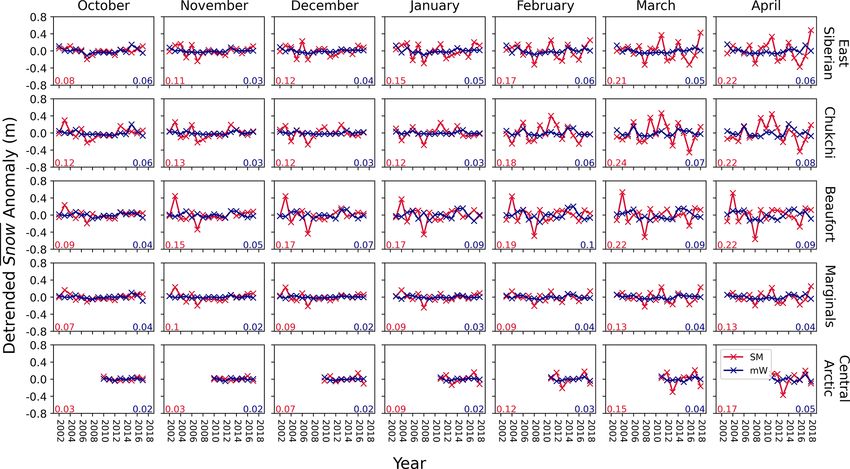
R. D. C. Mallett et al.: Snow’s impact on SIT variability and trends                                                              2433

Figure 2. (a) Tracks of Soviet drifting stations 3–31. (b) Number of days in each region in each month that snow stake measurements were
taken.

erate pan-Arctic snow-depth and density distributions. The            ucts. The SnowModel-LG data are provided on the same
sea ice motion vectors used were from the Polar Pathfinder            25 km EASE grid as the ESA-CCI radar freeboards described
data set at weekly time resolution (Tschudi et al., 2020).            above at daily time resolution. We averaged this daily prod-
SnowModel-LG exhibits more significant interannual vari-              uct to produce monthly gridded data for combination with
ability than mW99 in its output because it reflects year-to-          the monthly radar freeboard data.
year variations in weather and sea ice dynamics.
   SnowModel-LG includes a relatively advanced degree of              2.7   NASA Eulerian Snow on Sea Ice Model
physics in its modelling of winter snow accumulation. The                   (NESOSIM)
model creates and merges layers based on precipitation and
snowpack metamorphism. The effects of sublimation, depth-             To support and broaden the impact of our findings, we repeat
hoar formation and wind packing are included. However, the            our analyses with NESOSIM data from 2002–2015 (Petty
effects of snow loss to leads by wind and extra snow accumu-          et al., 2018b). NESOSIM data are released on a 100×100
lation due to sea ice roughness are not included. Furthermore,        km grid which was interpolated to the 25 × 25 km EASE
the heat flux to the snow is not sensitive to the thickness of        grid of the SnowModel-LG and radar freeboard data. NE-
the underlying sea ice.                                               SOSIM runs in a Eulerian framework and like SnowModel-
   SnowModel-LG creates a snow distribution based on re-              LG can assimilate precipitation data from a variety of reanal-
analysis data, and the accuracy of these snow data is un-             yses data. In contrast with SnowModel-LG’s multi-layered
likely to exceed the accuracy of the input. There is signifi-         scheme, NESOSIM uses a two-layer snow scheme to rep-
cant spread in the representation of the actual distribution of       resent depth-hoar and wind-packed layers. To define these
relevant meteorological parameters by atmospheric reanaly-            layers, it assimilates surface winds and temperature profiles
ses (Boisvert et al., 2018; Barrett et al., 2020). The results        from reanalysis. Wind-blown snow loss is parameterised to
of SnowModel-LG therefore depend on the reanalysis data               leads using daily sea ice concentration fields (Comiso, 2000,
set used. However, the data product used has been tuned to            updated 2017).
match Operation IceBridge (OIB)-derived snow depths dur-                 In this study we use data from a NESOSIM run initialised
ing spring time, and snow-depth differences between the re-           on 15 August for each year. The initial depth was produced
analysis products were found to be less than 5 cm (Stroeve            by a “near-surface air-temperature-based scaling of the Au-
et al., 2020). We note that the vast majority of Operation            gust W99 snow-depth climatology” (Petty et al., 2018b).
IceBridge flights were over the Beaufort Sea and the Green-           This is a linear scaling based on the duration of the preced-
landic side of the Central Arctic, which is generally cov-            ing summer melt season. Snow density was initialised using
ered by multi-year ice. It is therefore conceivable that the          the August snow-line observations of Soviet NP drifting sta-
scaling factors would be different if FYI were better sam-            tions 25, 26, 30 and 31. Data from the most recent publicly
pled by OIB. The time-averaged regional differences be-               available drifting stations were chosen to maximise their rel-
tween SnowModel-LG runs forced by ERA5 and MERRA2                     evance in a changing climate.
reanalysis data are shown in Fig. S3. The SnowModel-LG
data used in this study are generated from the average of
SnowModel-LG runs forced by the two reanalysis prod-

https://doi.org/10.5194/tc-15-2429-2021                                                      The Cryosphere, 15, 2429–2450, 2021
2434                                                     R. D. C. Mallett et al.: Snow’s impact on SIT variability and trends

3     Methods                                                      (1999) with those introduced by mW99 and SnowModel-LG
                                                                   at a given point. We carry out this analysis to establish that
3.1    Contributions to thickness determination from               the mW99 variability and trends at a given point (chosen as
       snow and radar freeboard data                               pixels on a 25 × 25 km EASE grid) are considerably smaller
                                                                   than those observed at drifting stations.
We now identify that the height correction due to slower              The monthly interannual variability (IAV) values pub-
radar pulse propagation in snow scales in almost direct pro-       lished in Warren et al. (1999) are calculated as the standard
portion to the total mass of penetrated snow (ms ; Fig. S1). As    deviation of the snow depths at drifting stations when com-
such, it can be easily combined with the change to the floe’s      pared to the climatology at the position of the stations. The
hydrostatic equilibrium from snow loading (also linearly de-       IAV values at a point-like drifting station in a region will
pendent on ms ) to make one transformation to modify Eq. (2)       therefore naturally be higher than the IAV of the region’s spa-
such that                                                          tial mean. As such, to compare IAV values from point-like
             ρw            ρw                                      drifting stations to mW99, we calculate the IAV at individual
SIT = fr           + ms          × 1.81 × 10⁻³ .             (3)
          ρw − ρi       ρw − ρi                                    ice-covered points on a 25 × 25 km equal-area grid (Brodzik
                                                                   et al., 2012). These are all positive values, which we then av-
   Physically, the first term of Eq. (3) corresponds to the SIT
                                                                   erage for comparison with the drifting stations. By regionally
were the sea ice known to have no snow cover. The second
                                                                   averaging the IAV values of many points rather than calcu-
term is the additional sea ice thickness that is inferred from
                                                                   lating the IAV of regional averages, we replicate the statistics
knowledge of the overlying snow cover. SIT has been decom-
                                                                   of the point-like drifting stations.
posed into linearly independent contributions from radar-
                                                                      However, the main part of this paper does not focus on
freeboard data and snow data. This allows the contributions
                                                                   trends and variability at a point (as measured by drifting sta-
of the two data components to SIT to be assessed indepen-
                                                                   tions) but instead investigates trends and variability in Snow
dently. A derivation of the 1.81×10⁻³ coefficient is available
                                                                   and SIT at the regional scale (Sect. 4.2 and 4.3). This vari-
in the Supplement.
                                                                   ability is significantly lower than the typical variability at a
   We highlight here that our expression in Eq. (3) of the con-
                                                                   point, as many local anomalies from climatology within a re-
tribution of snow data to SIT determination solely in terms
                                                                   gion are averaged out in the calculation of single, area-mean
of snow mass is technically convenient for using W99 to es-
                                                                   values which form a time series for each region.
timate sea ice thickness, as quadratic fits of density (unlike
depth and snow water equivalent) are not publicly available        3.3   Assessing regional interannual variability
for all months. This has led to the required density values of-
ten being set to a constant value or “backed out” by dividing      Section 4.2 of this paper focuses on the interannual variabil-
the published SWE distributions by the depth distributions.        ity in regional SIT, which (treating RF and Snow as random,
   Equation (3) and its factor of 1.81×10⁻³ allow the simple       dependent variables) can be expressed thus:
expression of the theoretical change to the radar freeboard         2      2     2
under rapid snow accumulation or removal. Making fr the            σSIT = σRF + σSnow + 2 Cov(RF, Snow),                       (6)
subject of the equation and assuming SIT constant we find
                                                                   where the final term represents the covariance between spa-
∂fr                                                                tially averaged radar freeboard and snow contributions. This
    = −1.81 × 10⁻³ (m/kgm−2 ).                              (4)    covariance term can be expressed as 2r ×σSnow ×σRF , where
∂ms
                                                                   r is the dimensionless correlation coefficient between the
We stress that the above equation assumes total radar pen-         variables and ranges between −1 and 1. To further explain
etration of overlying snow, an assumption discussed in             this term, if years of high RF are correlated with high Snow,
Sect. 5.3. As well as allowing independent analysis of the         then the covariance term will be high and interannual vari-
radar and snow data contributions to SIT at a point, the lin-      ability in SIT will be amplified. If mean snow depths are
early independent nature of Eq. (3) in terms of fr and ms          anti-correlated with mean radar freeboard across the years,
allows for a simple calculation of the average SIT in a region     interannual variability in SIT will be reduced.
(SIT) as                                                              SIT, RF and Snow were calculated where any valid grid
                                                                   points existed on the 25 × 25 km EASE grid. Because of this,
SIT = RF + Snow,                                            (5)    no average values were computed in the Kara Sea in October
where RF and Snow represent the spatial averages of the first      2009 or 2012. Furthermore, no October values were gener-
and second terms of Eq. (3).                                       ally available in the Barents Sea after 2008 (with the excep-
                                                                   tion of 2011 and 2014). The impact of this on our resulting
3.2    Assessing snow trends and variability at a point            analysis is clearly visible in the top left panel of Fig. 10. We
                                                                   do not exclude the Barents Sea in October from our analysis
In Sect. 4.1 we briefly compare the statistics for trends and      because of the low number of valid points, but we do high-
variability at drifting stations published in Warren et al.        light the undersampling issue here. We continue to consider

The Cryosphere, 15, 2429–2450, 2021                                                   https://doi.org/10.5194/tc-15-2429-2021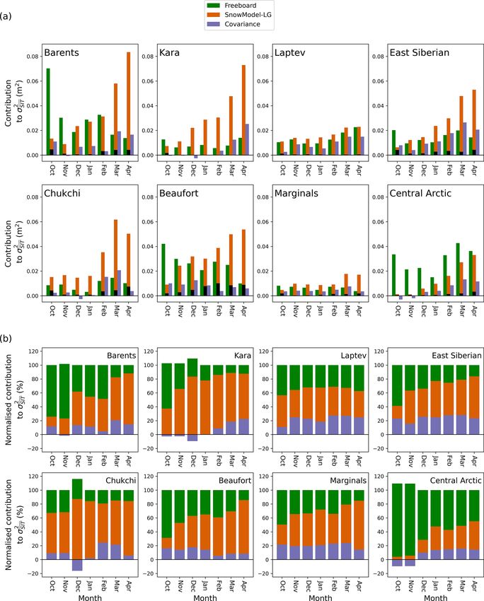
R. D. C. Mallett et al.: Snow’s impact on SIT variability and trends                                                        2435

it because we do not find statistically significant declining     0.05, with a null hypothesis of no trend. Trends were calcu-
trends with the data we have, so essentially we are report-       lated for regional SIT over the Envisat–CS2 period (2002–
ing a null result. Our calculations of interannual variability    2018) for all regions apart from the Central Arctic for which
in this month are inherently adjusted for the small sample        only CS2 data were available. We assess the relationship of
size, but we nonetheless urge caution in interpretation of the    these trends in SIT to trends in RF and Snow (Fig. S19).
values. The number of grid points available for averaging in         In Sect. 4.1.2 we show that basin-wide average snow depth
each region in each month are shown in Fig. S2.                   and SWE is decreasing in SnowModel-LG in most months
   The three terms on the right-hand side of Eq. (6) corre-       but only in October for mW99. We point out here that (under
spond to the three unique terms of the covariance matrix of       the paradigm of total radar wave penetration of snow on sea
the two terms of Eq. (5). The main-diagonal elements of this      ice) under-accounting for potential reductions in SWE may
2 × 2 matrix correspond to the variance of the snow contribu-     partially mask a decline in sea ice thickness, as reductions in
tion and the radar freeboard contribution to sea ice thickness,   radar freeboards are partially compensated for by reductions
terms one and two of Eq. (6). The off-diagonal elements are       in snow depths. From Eq. (5),
identical and sum to form the third term of Eq. (6).
   We calculated this matrix for each region in each month        ∂(SIT) ∂(RF) ∂(Snow)
                                                                        =     +        .                                      (7)
to investigate the sources of regional interannual variability      ∂t     ∂t     ∂t
in SIT for the time period under consideration (2002–2018).
The Central Arctic region is not sufficiently well observed       4     Results
by the Envisat radar altimeter (see Fig. 1), so the covariance
matrix for the region was only calculated for the CS2 period      4.1     Comparison of point trends and point variability
(2010–2018).
   In some cases a natural degree of covariance is introduced     4.1.1    Low interannual variability in mW99 compared
between the regional Snow and RF time series because they                  to drifting stations and SnowModel-LG
both display a decreasing trend. This “false variance” would
not be present were the system in a steady state. As such,        How does the variability in mW99 and SnowModel-LG at a
we detrended the regional time series prior to calculation of     given point compare to the values recorded at Soviet drifting
the covariance matrix. We found that doing this significantly     stations published by Warren et al. (1999)? These values for
decreased the value of the covariance term in Eq. (6).            interannual variability are not currently used in sea ice thick-
   We consider the relative contributions of these three terms    ness retrievals (although they do contribute to uncertainty es-
to σ 2 in calculations involving mW99 and SnowModel-              timates in the ESA-CCI sea ice thickness product). Nonethe-
     SIT
LG (Sect. 4.2). In light of these results, we then re-assess      less, they offer a benchmark against which to evaluate the
the statistical significance of regional trends in SIT using      variability induced by mW99 at a given location.
SnowModel-LG.                                                        Using the method described in Sect. 3.2 we find that the
   Detection of temporal trends in SIT is critically dependent    snow variability at a point from mW99 (Fig. 3, blue bars) is
on accurate characterisation of σ 2 . This is because con-        on average about 50 % of the values recorded at the drifting
                                    SIT
ventional tests for trend exploit the known probability of a      stations (Fig. 3, green bars). By comparison, SnowModel-LG
system with no trend generating the data at hand through          snow-depth variability at a given point is significantly higher,
variability alone (Chandler and Scott, 2011, p. 61). In this      ranging from ∼ 75 % of the drifting station values in October
paper we argue that the σ 2        term of Eq. (6) has been       to ∼ 115 % by the end of winter.
                             Snow
systematically underestimated through the use of a quasi-            We present this analysis of the point-like snow variability
climatological snow data set (mW99). As an alternative to         to illustrate that mW99 does not introduce enough variabil-
this we use the results of SnowModel-LG, a snow accumula-         ity at a given point to match that observed at drifting stations
tion model that incorporates interannual changes in precipi-      from year to year. Furthermore, the variability that does exist
tation amount, freeze-up timing and sea ice distribution.         is confined to a distinct band of the Arctic Ocean (Fig. 4).
                                                                  This band represents areas where the sea ice type is not typ-
3.4   Assessing regional temporal trends                          ically either FYI or MYI. Instead it is either switching be-
                                                                  tween the two, or it is an area where FYI has replaced MYI
In Sect. 4.3 we examine temporal trends in regional SIT for       during the period of analysis. In areas where sea ice type is
each month of the growth season (October–April) and de-           temporally unchanging, snow variability is not present. This
compose the results by sea ice type. It is stressed that these    has implications at the regional scale as marginal seas with a
regional trends are each the trend of a single time series of     consistent sea ice type experience unrealistically low σSnow
spatially averaged thickness values rather than the average of    in the mW99 scheme.
many trends in sea ice thickness at various pixels in a region.
Regional trends were deemed statistically significant if they
passed a two-tailed hypothesis test with a p value less than

https://doi.org/10.5194/tc-15-2429-2021                                                The Cryosphere, 15, 2429–2450, 2021
2436                                                          R. D. C. Mallett et al.: Snow’s impact on SIT variability and trends

Figure 3. Interannual variability (2002–2018) in snow depth from mW99 and SnowModel-LG compared to the values given in Table 1 of
Warren et al. (1999).

Figure 4. mW99 snow-depth variability at each EASE grid point over the 2002–2018 period. This is calculated by generating a time series
of snow depth at each point and then calculating the standard deviation of that time series. High variability is displayed in a band where sea
ice type typically fluctuates from year to year. IAV is zero in areas that do not exhibit sea ice type variability, introducing unphysically low
variability in SIT.

4.1.2   Lack of temporal trends in mW99 compared to                       depth is in part due to the diminishing area of October FYI
        SnowModel-LG and in situ data                                     relative to that of MYI (Fig. S4) and in part due to the retreat
                                                                          of the October sea ice into the Central Arctic where W99 ex-
Weak trends exist at some points in the mW99 Arctic snow                  hibits higher snow depths and SWE. The increasing October
distribution due to the shifting distribution and abundance of            areal dominance of MYI is in part driven by delayed Arctic
first-year ice in the Arctic. In this section we briefly address          freeze-up (Markus et al., 2009; Stroeve et al., 2014). The area
their size, sign and veracity, leaving regional analysis until            of sea ice over which the W99 climatology is halved in Octo-
Sect. 4.2.                                                                ber is therefore shrinking, and basin-wide mean snow depths
   Values for SWE and depth trends measured by individ-                   in mW99 are increasing. Trends in sea ice type fraction for
ual drifting stations are given in W99, but the values are not            each winter month are displayed in Fig. S4, and monthly time
statistically significant for any of the winter months and as             series for mW99 SWE are displayed in Fig. S5.
such are not displayed here. We instead compare the point                    Unlike mW99, SnowModel-LG exhibits statistically sig-
trends at all colour-coded regions of Fig. 1 from mW99 and                nificant, negative point trends for the later 5 of the 7 win-
SnowModel-LG (Fig. 5).                                                    ter months (when averaged at a basin-wide scale). We iden-
   We find that when we average the point trends at a basin-              tify two processes as responsible for this decreasing trend:
wide scale, the only statistically significant trend (at the 5 %          the MYI area is shrinking, so a smaller MYI sea ice area
level) for mW99 snow depth is a positive one for the month of             is present during the high snowfall months of September
October (+0.11 cm/yr; Fig. 5). This increasing trend in snow              and October (Boisvert et al., 2018); and also freeze-up com-

The Cryosphere, 15, 2429–2450, 2021                                                             https://doi.org/10.5194/tc-15-2429-2021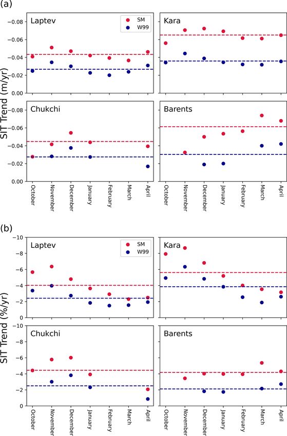
R. D. C. Mallett et al.: Snow’s impact on SIT variability and trends                                                            2437

Figure 5. Basin-wide spatial average of point-like trends in (a) snow depth and (b) SWE, from mW99 and SnowModel-LG. Calculated
for the Envisat–CS2 period (2002–2018). Significance values (in %) are given at the base of each bar. Only October trends for mW99 are
significant at the 5 % level, whereas significant negative trends exist in SnowModel-LG for December–April.

mences later, so a lower FYI area is available in these              Fig. 1. SnowModel-LG data produce more variable time se-
months, and more precipitation falls directly into the ocean.        ries of Snow (i.e. higher values of σ 2 ; cf. Eq. 6). This is
                                                                                                            Snow
Webster et al. (2014) observed a −0.29 cm/yr trend in West-          the case for all months, in all regions. For snow in the Kara
ern Arctic spring snow depths using both airborne and in             Sea, mW99 introduces almost 4 times less interannual vari-
situ sources. These airborne contributions to this statistic in-     ability into SIT via Snow than SnowModel-LG in the April
cluded data over both sea ice types, and the in situ con-            time series. This analysis is further broken down by sea ice
tributions included data from individual Soviet drifting sta-        type in Figs. S7 and S8.
tions from the Western Arctic. The statistic compares well              Having shown that SnowModel-LG’s contribution to SIT
with the behaviour of SnowModel-LG (−0.27 cm/yr March;               is more variable than mW99, how does this increased vari-
−0.31 cm/yr April) but is considerably beyond that of the            ability propagate into sea ice thickness variability itself
non-statistically significant trends of W99 and mW99.                (σ 2 )? To answer this question, we must examine the way
                                                                        SIT
   What might the effects of this decline be on SIT at re-           in which the snow contribution to SIT combines with data
gional scales and larger? In terms of Eq. (7), models and            from satellite radar freeboard measurements. Having calcu-
observations indicate that ∂(Snow)/∂t is negative on long            lated the σ 2    term of Eq. (6) (displayed in Fig. 6), we now
                                                                                Snow
timescales (Webster et al., 2014; Warren et al., 1999; Stroeve       turn to the 2 Cov(RF, Snow) term. To assess this we calcu-
et al., 2020). However, the use of mW99 effectively sets             late the magnitude and statistical significance of correlations
∂(Snow)/∂t to zero and to a positive value in October. This          between the detrended RF and Snow contributions to SIT in
has the effect of biasing ∂(SIT)/∂t high (and towards zero).         individual years, regions and months.
Section 4.3 examines the effect of using SWE data with a                To do this we calculated a monthly time series of RF and
more realistic decline on regional SIT trends; this is medi-         Snow for each region over the time period 2002–2018 (with
ated by the effects of higher interannual variability, which is      the Central Arctic being 2010–2018). Because we consid-
examined in Sect. 4.2.                                               ered eight regions and 7 months, this led to 56 pairs of time
                                                                     series for RF and Snow. We then detrended each of them. We
4.2   Realistic SWE interannual variability enhances                 then calculated the correlation between each of the pairs of
      regional SIT interannual variability                           detrended time series. We note here that the correlation be-
                                                                     tween the time series is dependent on their relative position to
Having illustrated the deficiency of point trends and point          a linear regression. These correlation statistics are thus inde-
variability in mW99, we now move on to the impact of snow            pendent of the absolute magnitude of the values, their units or
data on SIT at the regional scale.                                   any linear scaling of the axes. We therefore choose to present
   We calculate the interannual variability of detrended time        the correlations in Fig. 7 without axes and scaled to the rect-
series of the snow contribution to the thickness determina-          angular panels, so as to best show the relative positions of the
tion (Snow) from mW99 and SnowModel-LG. We display                   points without extraneous numerical information.
some of these results in Fig. 6. We did this for every win-
ter month (October–April) and for each region defined in

https://doi.org/10.5194/tc-15-2429-2021                                                    The Cryosphere, 15, 2429–2450, 2021
2438 R. D. C. Mallett et al.: Snow’s impact on SIT variability and trends
Figure 6. Detrended time series of spatially averaged snow contributions to sea ice thickness (Snow) by region from W99 (blue) and
SnowModel-LG (red). Standard deviation values are displayed for SnowModel-LG (lower left, red) and mW99 (lower right, blue). All
regions are plotted in Supplement Fig. S6.
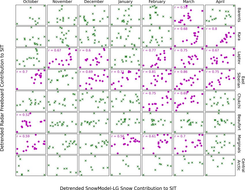
We find statistically significant correlations between Snow some areas, which introduces an inherent correlation from
and RF to generally range between 0.6–0.85 (Fig. 7). All sta- the trend.
tistically significant correlations were positive ones, and this Having identified and quantified regions and months of
was also the case when individual sea ice types were consid- significant covariance between Snow and RF (Fig. 7), we
ered for each region. When all sea ice types were considered, are in a position to fully answer the question of how the in-
the Laptev and East Siberian seas exhibited statistically sig- creased variability of SnowModel-LG over mW99 (shown in
nificant correlations in 5 and 6 of the 7 growth-season months Fig. 6) ultimately impacts σ 2 . We plot the three contribut-
SIT
respectively. The Barents Sea and the Beaufort Sea both ex- ing components to σ 2 for each region in each winter month
SIT
hibited 1 month of correlation, and the Central Arctic region (Fig. 8). We note that in the case of negative covariability be-
exhibited no months of correlation – the reasons for this are tween Snow and RF, it is possible for σ 2 +σRF 2 to be larger
Snow
discussed in Sect. 5.4). When analysed as a single, large re-
than σ 2 . This is not problematic because σ 2 + σRF 2 does
gion, the marginal seas area exhibits correlations in 4 of the SIT Snow
not represent a real quantity when the variables are not inde-
7 months analysed, with the strength of these correlations in-
pendent.
creasing over the season.
In the marginal seas σ 2 2 to become the
overtakes σRF
We continued this analysis by breaking down the regions Snow
by sea ice type. The area of the Central Arctic sea ice covered main constituent of σ 2 by the end of the growth season
SIT
with first-year ice exhibits strong correlations (all above 0.8) (Fig. 8). This is particularly driven by the behaviour of the
in the later 5 months of the winter (Fig. S9). Beaufort and East Siberian seas, where this relationship is
clearly visible. In the Central Arctic σRF2 narrowly remains
When considering correlations over multi-year ice (MYI),
the marginal seas grouping exhibits correlations in the first 4 the dominant component of σ 2 throughout the cold season,
SIT
growth-season months (Fig. S10). The MYI fraction Central although σ 2 plays an increasing role as the season pro-
Snow
Arctic, Chukchi and Barents seas exhibited no correlations. gresses.
We note that this analysis is relatively sensitive to the de- Covariance between RF and Snow makes relatively con-
trending process. When performed without detrending, sta- stant contributions to σ 2 of the marginal seas grouping in
SIT
tistically significant correlations are noticeably more com- comparison to the other two components, but analysis of
mon. This is because Snow and RF are both in decline in this grouping conceals more significant variation at the scale
The Cryosphere, 15, 2429–2450, 2021 https://doi.org/10.5194/tc-15-2429-2021R. D. C. Mallett et al.: Snow’s impact on SIT variability and trends 2439 Figure 7. Covariability of contributions to sea ice thickness from radar freeboard and SnowModel-LG-derived snow components over all sea ice types. Plots are coloured with magenta when a statistically significant correlation is present between the contributions (p > 0.95). Analogous plots are displayed for the FYI and MYI components of the regions in Figs. S9 and S10. of the individual group members. The covariability term of and 0.16 m with SnowModel-LG. This represents an increase Eq. (6) makes a larger contribution than radar freeboard in SIT variability of 77 %. For the Central Arctic this figure is variability itself at times, for example in the Kara and East considerably smaller, at 25 %. When the individual marginal Siberian seas at the end of winter and for the Chukchi Sea seas are considered, the largest increase was the Kara Sea in February and March. For the Central Arctic, the covari- (138 %) and the smallest was the Beaufort Sea (35 %). ability term generally makes less of a contribution to total One key aspect of interannual variability is how it com- SIT variability than radar freeboard or snow variability indi- pares to typical values. When IAV is expressed as a percent- vidually and is negative in the first 2 months of winter. We age of the regional mean thickness, the Barents Sea exhibits note that the covariability is almost always positive in the the largest increase when calculated with SnowModel-LG: marginal seas with the exception of December in the Kara the standard deviation (as a percentage of mean thickness) and Chukchi seas. increases from 15 % to 25 %. When variability is viewed in Finally, we directly compare the variability of SIT itself, this way, the increase in the Central Arctic is small (7.9 % when calculated using SnowModel-LG and mW99. We con- to 9.4 %). Variability as a fraction of mean thickness is also duct this exercise in both absolute terms (Fig. 9a) and as a highest in the Barents Sea when calculated with SnowModel- fraction of the regional mean thickness (Fig. 9b). LG – whereas with mW99 this designation would go to the Calculation of regional SIT with SnowModel-LG reveals Beaufort Sea. When analysed as one area, variability (as a higher variability in all marginal seas of the Arctic Basin in fraction of mean thickness) in the marginal seas transitions all months. When the marginal seas are analysed as a con- from being 7.5 % of the mean thickness to 13.8 % when cal- tiguous entity, the standard deviation is 0.09 m with mW99 culated with SnowModel-LG. https://doi.org/10.5194/tc-15-2429-2021 The Cryosphere, 15, 2429–2450, 2021
2440                                                         R. D. C. Mallett et al.: Snow’s impact on SIT variability and trends

Figure 8. Constituent parts of σ 2    of different regions. Bars represent the variance (σ 2 ) of RF and Snow and the covariance between the
                                SIT
two. Panel (a) illustrates the absolute variance contributions, and panel (b) illustrates the relative contributions. The variance of Snow in
mW99 is indicated in panel (a) by a superimposed black bar. Snow contributes significantly more variability in the late winter than radar
freeboard in most of the marginal seas.

   We also note that MYI exhibits more thickness variability             sea ice types is highly similar (with FYI IAV slightly larger
than FYI (both absolutely and relative to the sea ice type’s             when calculated relative to regional mean thickness).
mean thickness) in all the marginal seas (Fig. S11). For the
marginal seas as a single group, MYI is roughly twice as
variable in absolute terms. This is not the case in the Cen-
tral Arctic, where the thickness variability of the individual

The Cryosphere, 15, 2429–2450, 2021                                                           https://doi.org/10.5194/tc-15-2429-2021
R. D. C. Mallett et al.: Snow’s impact on SIT variability and trends 2441
Figure 9. Standard deviation in sea ice thickness over the period 2002–2018 except for the Central Arctic: 2010–2018 (a) calculated in
absolute terms and (b) calculated as a percentage of the regional mean thickness over the period. Mean growth-season values shown with
dashed lines. The individual detrended regional time series from which this figure is synthesised are available in Fig. S12.
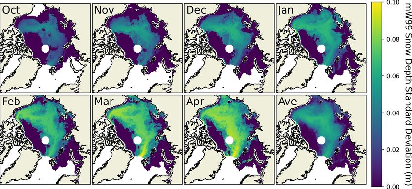
4.3 New and faster thickness declines in the marginal in April, where the decline rate increased by a factor of 2.1.
seas When analysed as an aggregated area and with mW99, the to-
tal marginal seas area exhibits a statistically significant neg-
As well as exhibiting higher interannual variability than ative trend in November, December, January and April. The
mW99, SnowModel-LG Snow values decline over time in East Siberian Sea is the only region to have a month of de-
most regions due to decreasing SWE values year over year. cline when calculated with mW99 but not with SnowModel-
Here we examine the aggregate contribution of a more vari- LG.
able but declining Snow time series in determining the mag- We now turn our attention to new trends that stem from the
nitude and significance of trends in SIT. use of SnowModel-LG over mW99 (Fig. 10; red panels). Our
We first assess regions where SIT was already in statisti- analysis reveals a new, statistically significant SIT decline in
cally significant decline when calculated with mW99. This the Chukchi Sea in October (taking the number of months
is the case for all months in the Laptev and Kara seas and 4 with a decline in SIT to 5). Perhaps more significantly, the
of 7 months in the Chukchi and Barents sea. The rate of de- aggregated marginal seas region exhibits 2 new months of
cline in these regions grew significantly when calculated with statistically significant declining SIT in October and Febru-
SnowModel-LG data (Fig. 10; green panels). Relative to the ary, taking the total number of declining months to 6. No
decline rate calculated with mW99, this represents average months in any marginal sea exhibited a statistically signifi-
increases of 62 % in the Laptev sea, 81 % in the Kara Sea cant increasing trend in SIT (with either snow data set).
and 102 % in the Barents Sea. The largest increase in an al- The Central Arctic region exhibits a statistically signifi-
ready statistically significant decline was in the Chukchi Sea cant thickening October trend with both snow data sets (10
https://doi.org/10.5194/tc-15-2429-2021 The Cryosphere, 15, 2429–2450, 20212442 R. D. C. Mallett et al.: Snow’s impact on SIT variability and trends
and 9 cm/yr with SnowModel-LG and mW99). The region calculated with mW99, and this is also true to a lesser extent
exhibits an additional month of increase in November when in the Chukchi Sea.
calculated with SnowModel-LG (7 cm/yr).
We also analyse these regional declines as a percentage of
the regional mean sea ice thickness in the observational pe- 5 Discussion
riod (2002–2018; Fig. 11). We observe the average growth-
season thinning to increase from 21 % per decade to 42 % 5.1 Sensitivity of findings to choice of snow product
per decade in the Barents Sea, 39 % to 56 % per decade in
5.1.1 Choice of climatology – combining AMSR2 with
the Kara Sea, and 24 % to 40 % per decade in the Laptev Sea
mW99
when using SnowModel-LG instead of mW99. Five of the 7
growth-season months in the Chukchi Sea exhibit a decline The most recent sea ice thickness product from the Alfred
with SnowModel-LG of (on average) 44 % per decade. This Wegener Institute (Hendricks and Ricker, 2019) makes use
is much more than that of the 4 significant months observ- of a new snow climatology, generated by the merging of W99
able with mW99 (25 % per decade). We find the marginal with snow-depth data derived from the AMSR2 passive mi-
seas (when considered as a contiguous, aggregated group) crowave record. This is then applied with a halving scheme
to be losing 30 % of its mean thickness per decade in the based on sea ice type in a similar way to mW99 (but with the
6 statistically significant months when SIT is calculated us- AMSR2 component not halved). This likely improves the ab-
ing SnowModel-LG (as opposed to mW99). solute accuracy of snow depths (and thus sea ice thickness)
We further analyse these declining trends by sea ice type. but does not resolve the issues discussed in this paper involv-
This reveals the aggregate trends in the marginal seas to be ing trends and variability. The modified AMSR2/W99 cli-
broadly driven by thickness decline in FYI rather than MYI. matology functions in a very similar way to mW99 – a weak
We note that the FYI sea ice cover in the Kara and Laptev IAV is introduced in areas of interannually fluctuating sea
seas is in statistically significant decline with either snow ice type. Any trends will be the result of trends in the relative
product in all months. The FYI cover in the Barents Sea is dominance of sea ice type. This was discussed in Sect. 4.1.2
also in decline for 6 of the 7 winter months when calcu- and illustrated in Fig. S4: sea ice type trends are only signif-
lated with SnowModel-LG. We find that (when analysed with icant in October and January, where they are weak.
SnowModel-LG) if any month in a specific marginal sea is in
“all types” decline, its first-year ice is also statistically signif- 5.1.2 Choice of reanalysis forcing for SnowModel-LG
icantly declining.
Barrett et al. (2020) reviewed precipitation data from vari-
ous reanalysis products over the Arctic Ocean using records
4.4 Changes to the sea ice thickness distribution and
from the Soviet drifting stations and found the magnitude of
seasonal growth
interannual variability to be similar. They further broke these
data down to the regional scale using the same regional def-
We now consider differences in the spatial sea ice thick- initions in this paper and found that this similarity persisted.
ness distribution introduced by a snow product with IAV. Be- Boisvert et al. (2018) conducted a similar analysis with drift-
cause mW99 has low spatial variability in its SWE fields (the ing ice mass balance buoys and found the interannual vari-
quadratic fits are relatively flat), it produces a more sharply ability of the data sets to also be similar (although the au-
peaked and narrow SIT distribution with lower probabilities thors found larger discrepancies in magnitude). These differ-
of thinner or thicker sea ice in the months January–April. The ences in magnitude however cannot be physical (as there is
SIT distribution also exhibits some degree of bimodality due only one Arctic), and Cabaj et al. (2020) were able to bring
to the halving scheme. This bimodality is to a large degree precipitation estimates into better alignment using Cloud-
represented in the SnowModel-LG histograms – an encour- Sat data with a scaling approach. However this scaling ap-
aging result (Fig. S13). proach preserved the interannual variability of the data sets,
The regional, seasonal growth rate is also similar when which Barrett et al. (2020) and Boisvert et al. (2018) found
comparing calculations with SnowModel-LG and mW99 to be in comparatively good agreement. To investigate how
(Fig. S14). These rates were calculated over the period 2002– this variability propagates into Snow variability, we calculate
2018 with the exception of the Central Arctic, which was re- Snow time series from SnowModel-LG runs forced by both
stricted to the period 2010–2018. Among the most salient dif- MERRA-2 and ERA-5 data and find their variability to be
ferences are the much smoother seasonal evolution of snow very similar (Fig. S15).
cover in the Barents Sea from SnowModel-LG and the de- With regard to trends, we find that the two different reanal-
cline in SWE from March to April in the Kara, Laptev and ysis forcings generally introduce minimal differences in the
Beaufort seas with mW99 (compared to a continued increase SIT trends (Fig. S16). We do however find that small differ-
with SnowModel-LG). In the East Siberian and Laptev seas ences in SWE cause the Snow contribution of the MERRA-2
there is clearly a slightly lower seasonal growth rate when SnowModel-LG run to exhibit statistically significant decline
The Cryosphere, 15, 2429–2450, 2021 https://doi.org/10.5194/tc-15-2429-2021You can also read