A crash-testing framework for predictive uncertainty assessment when forecasting high flows in an extrapolation context
←
→
Page content transcription
If your browser does not render page correctly, please read the page content below
Hydrol. Earth Syst. Sci., 24, 2017–2041, 2020
https://doi.org/10.5194/hess-24-2017-2020
© Author(s) 2020. This work is distributed under
the Creative Commons Attribution 4.0 License.

A crash-testing framework for predictive uncertainty assessment
when forecasting high flows in an extrapolation context
Lionel Berthet1 , François Bourgin2,3 , Charles Perrin3 , Julie Viatgé3 , Renaud Marty1 , and Olivier Piotte4
1 DREAL    Centre-Val de Loire, Loire Cher & Indre Flood Forecasting Service, Orléans, France
2 GERS-LEE,    Univ Gustave Eiffel, IFSTTAR, 44344 Bouguenais, France
3 Université Paris-Saclay, INRAE, UR HYCAR, 92160 Antony, France
4 Ministry for the Ecological and Inclusive Transition, SCHAPI, Toulouse, France

Correspondence: Lionel Berthet (lionel.berthet@developpement-durable.gouv.fr)

Received: 18 April 2019 – Discussion started: 7 May 2019
Revised: 13 January 2020 – Accepted: 15 March 2020 – Published: 23 April 2020

Abstract. An increasing number of flood forecasting ser-          mation or the Box–Cox transformation can be a reasonable
vices assess and communicate the uncertainty associated           choice for flood forecasting.
with their forecasts. While obtaining reliable forecasts is a
key issue, it is a challenging task, especially when forecast-
ing high flows in an extrapolation context, i.e. when the event
magnitude is larger than what was observed before. In this        1     Introduction
study, we present a crash-testing framework that evaluates
the quality of hydrological forecasts in an extrapolation con-    1.1    The big one: dream or nightmare for the
text. The experiment set-up is based on (i) a large set of               forecaster?
catchments in France, (ii) the GRP rainfall–runoff model de-
signed for flood forecasting and used by the French opera-        In many countries, operational flood forecasting ser-
tional services and (iii) an empirical hydrologic uncertainty     vices (FFS) issue forecasts routinely throughout the year
processor designed to estimate conditional predictive uncer-      and during rare or critical events. End users are mostly con-
tainty from the hydrological model residuals. The variants        cerned by the largest and most damaging floods, when crit-
of the uncertainty processor used in this study differ in the     ical decisions have to be made. For such events, operational
data transformation they use (log, Box–Cox and log–sinh) to       flood forecasters must get prepared to deal with extrapola-
account for heteroscedasticity and the evolution of the other     tion, i.e. to work on events of a magnitude that they and their
properties of the predictive distribution with the discharge      models have seldom or never met before.
magnitude. Different data subsets were selected based on             The relevance of simulation models and their calibration
a preliminary event selection. Various aspects of the prob-       in evolving conditions, such as contrasted climate conditions
abilistic performance of the variants of the hydrologic un-       and climate change, has been studied by several authors.
certainty processor, reliability, sharpness and overall quality   For example, Wilby (2005), Vaze et al. (2010), Merz et al.
were evaluated. Overall, the results highlight the challenge of   (2011) and Brigode et al. (2013) explored the transferabil-
uncertainty quantification when forecasting high flows. They      ity of hydrological model parameters from one period to an-
show a significant drop in reliability when forecasting high      other and assessed the uncertainty associated with this pa-
flows in an extrapolation context and considerable variabil-      rameterisation, while Coron et al. (2012) proposed a gener-
ity among catchments and across lead times. The increase in       alisation of the differential split-sample test (Klemes̆, 1986).
statistical treatment complexity did not result in significant    In spite of its importance in operational contexts, only a few
improvement, which suggests that a parsimonious and easily        studies have addressed the extrapolation issue for flow fore-
understandable data transformation such as the log transfor-      casting, to the best of our knowledge, with the notable ex-
                                                                  ception of data-driven approaches (e.g. Todini, 2007). Im-

Published by Copernicus Publications on behalf of the European Geosciences Union.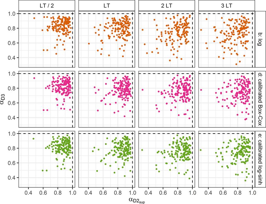
2018                                                   L. Berthet et al.: Uncertainty assessment when forecasting high flows

rie et al. (2000), Cigizoglu (2003) and Giustolisi and Lau-        To achieve reliable forecasts, a correct description of the het-
celli (2005) evaluated the ability of trained artificial neural    eroscedasticity, either explicitly or implicitly, is necessary.
networks (ANNs) to extrapolate beyond the calibration data            Various approaches to uncertainty assessment have been
and showed that ANNs used for hydrological modelling may           developed to assess the uncertainty in hydrological predic-
have poor generalisation properties. Singh et al. (2013) stud-     tions (see e.g. Montanari, 2011). The first step consists of
ied the impact of extrapolation on hydrological prediction         identifying the different sources of uncertainty or at least the
with a conceptual model, and Barbetta et al. (2017) expressed      most important ones that have to be taken into account given
concerns for the extrapolation context defined as floods of a      a specific context. In the context of flood forecasting, decom-
magnitude not encountered during the calibration phase.            posing the total uncertainty into its two main components
   Addressing the extrapolation issue involves a number of         is now common: the input uncertainty (mainly the meteoro-
methodological difficulties. Some data issues are specific to      logical forecast uncertainty) and the modelling uncertainty,
the data used for hydrological modelling, such as the rat-         as proposed by Krzysztofowicz (1999). More generally, the
ing curve reliability (Lang et al., 2010). Other well-known        predictive uncertainty due to various sources may be explic-
issues are related to the calibration process: are the param-      itly modelled and propagated through the modelling chain,
eters, which are calibrated on a limited set of data, repre-       while the “remaining” uncertainty (from the other sources)
sentative or at least somewhat adapted to other contexts? A        may then be assessed by statistical post-processing.
robust modelling approach for operational flood forecasting,
i.e. a method able to provide relevant forecasts in conditions     1.2.1   Modelling each source of uncertainty
not met during the calibration phase, requires paying spe-
cial attention to the behaviour of hydrological models and         A first approach intends to model each source of uncertainty
the assessment of predictive uncertainty in an extrapolation       separately and to propagate these uncertainties through the
context.                                                           modelling chain (e.g. Renard et al., 2010). Following this
                                                                   approach, the predictive uncertainty distribution results from
1.2    Obtaining reliable forecasts remains a challenging          the separate modelling of each relevant source of uncertainty
       task                                                        (e.g. in their study on hydrological prediction, Renard et al.
                                                                   (2010) did not have to consider the uncertainty in meteo-
Even if significant progress has been made and implemented         rological forecasts) and from the statistical model specifi-
in operational flood forecasting systems (e.g. Bennett et al.,     cation. While this approach is promising, operational appli-
2014; Demargne et al., 2014; Pagano et al., 2014), some un-        cation can be hindered by the challenge of making the hy-
certainty remains. In order to achieve efficient crisis man-       drological modelling uncertainty explicit, as pointed out by
agement and decision making, communication of reliable             Salamon and Feyen (2009).
predictive uncertainty information is therefore a prerequi-           In practice, it is necessary to consider the meteorological
site (Todini, 2004; Pappenberger and Beven, 2006; Demeritt         forecast uncertainty to issue hydrological forecasts. The en-
et al., 2007; Verkade and Werner, 2011). Hereafter, reliability    semble approaches intend to account for this source of uncer-
is defined as the statistical consistency between the observa-     tainty. They are increasingly popular in the research and the
tions and the predictive distributions (Gneiting et al., 2007).    operational forecasting communities. An increasing number
   The uncertainty associated with operational forecasts is        of hydrological ensemble forecasting systems are in opera-
most often described by a predictive uncertainty distribu-         tional use and have proved their usefulness, e.g. the Euro-
tion. Assessing a reliable predictive uncertainty distribution     pean Flood Awareness System (EFAS; Ramos et al., 2007;
is challenging because hydrological forecasts yield residu-        Thielen et al., 2009; Pappenberger et al., 2011; Pappenberger
als that show heteroscedasticity, i.e. an increase in the uncer-   et al., 2016) and the Hydrologic Ensemble Forecast Service
tainty variance with discharge, time autocorrelation, skew-        (HEFS; e.g. Demargne et al., 2014).
ness etc. Some studies (e.g. Yang et al., 2007b; Schoups and          Multi-model approaches can be used to assess modelling
Vrugt, 2010) account for these properties for the calibration      uncertainty (Velazquez et al., 2010; Seiller et al., 2017).
of hydrological models within a Bayesian framework, using          While promising, this approach requires the implementation
specific formulations of likelihood. In an extrapolation con-      and the maintenance of a large number of models, which can
text, it is of utter importance that the predictive uncertainty    be burdensome in operational conditions. There is no evi-
assessment provides a correct description of the evolution of      dence that such an approach ensures that the heteroscedas-
the predictive distribution properties with the discharge mag-     ticity of the predictive uncertainty distribution would be cor-
nitude. Bremnes (2019) showed that the skewness of wind            rectly assessed.
speed distribution depends on the forecasted wind. Mod-               In forecasting mode, data assimilation schemes based on
elled residuals of discharge forecasts often exhibit high het-     statistical modelling are of common use to reduce and as-
eroscedasticity (Yang et al., 2007a). McInerney et al. (2017)      sess the predictive uncertainty. Some algorithms such as par-
focused their study on representing error heteroscedasticity       ticle filters (Moradkhani et al., 2005a; Salamon and Feyen,
of discharge forecasts with respect to simulated streamflow.       2009; Abbaszadeh et al., 2018) or the ensemble Kalman filter

Hydrol. Earth Syst. Sci., 24, 2017–2041, 2020                                    www.hydrol-earth-syst-sci.net/24/2017/2020/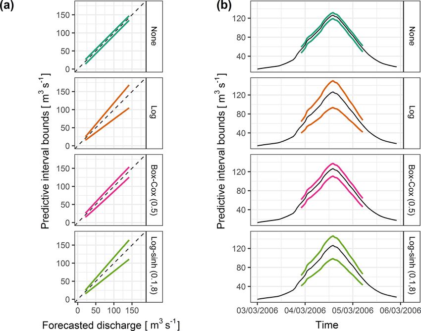
L. Berthet et al.: Uncertainty assessment when forecasting high flows                                                         2019

(Moradkhani et al., 2005b) provide an assessment of the pre-           Note that many of these approaches use a variable transfor-
dictive uncertainty as a direct result of data assimilation (“in    mation to handle the heteroscedasticity and more generally
the loop”). Some of these approaches can explicitly account         the evolution of the predictive distribution properties with
for the desired properties of the predictive uncertainty dis-       respect to the forecasted discharge. Some have no calibrated
tribution, such as heteroscedasticity, through the likelihood       parameter, while others encompass a few calibrated param-
formulation.                                                        eters, allowing more flexibility in the predictive distribution
                                                                    assessment. More details on commonly used variable trans-
1.2.2   Post-processing approaches                                  formations are presented in Sect. 2.1.4.
Alternatively, numerous post-processors of deterministic or         1.3   Scope
probabilistic models have been developed to account for the
uncertainty from sources that are not modelled explicitly.          In this article, we focus on uncertainty assessment with
They differ in several aspects (see a recent review by Li et al.,   a post-processing approach based on residuals modelling.
2017). Most approaches are conditional: the predictive uncer-       While the operational goal is to improve the hydrological
tainty is modelled with respect to a predictor, which most of-      forecasting, this study does not consider the meteorological
ten is the forecasted value (Todini, 2007, 2009). Some meth-        forecast uncertainty: it only focuses on the hydrological mod-
ods are based on predictive distribution modelling, while oth-      elling uncertainty, as these two main sources of uncertainty
ers can be described as “distribution-free”, as mentioned by        can be considered independently (e.g. Bourgin et al., 2014).
Breiman (2001). Among the former, many approaches are               Del Giudice et al. (2013) and McInerney et al. (2017) pre-
built in a statistical regression framework to assess the total     sented interesting comparisons of different variable transfor-
or remaining predictive uncertainty. Examples are the hydro-        mations used for residuals modelling. Yet, their studies do
logic uncertainty processor (HUP) in a Bayesian forecasting         not focus on the extrapolation context. Since achieving a re-
system (BFS) framework (Krzysztofowicz, 1999; Krzyszto-             liable predictive uncertainty assessment in an extrapolation
fowicz and Maranzano, 2004), the model-conditional pro-             context is a challenging task likely to remain imperfect if the
cessor (MCP; Todini, 2008; Coccia and Todini, 2011; Bar-            stability of the characteristics of the predictive distributions
betta et al., 2017), the meta-Gaussian model of Montanari           is not properly ensured, it requires a specific crash-testing
and Grossi (2008) or the Bayesian joint probability (BJP)           framework (Andréassian et al., 2009). The objectives of this
method (Wang et al., 2009), among others. The latter ap-            article are
proaches build a description of the predictive residuals from
past error series, such as data-learning algorithms (Solo-            – to present a framework aimed at testing the hydrological
matine and Shrestha, 2009). Some related methods are the                modelling and uncertainty assessment in the extrapola-
non-parametric approach of Van Steenbergen et al. (2012),               tion context,
the empirical hydrological uncertainty processor of Bour-             – to assess the ability and the robustness of a post-
gin et al. (2014) or the k-nearest neighbours method of                 processor to provide reliable predictive uncertainty as-
Wani et al. (2017). The quantile regression (QR) framework              sessment for large floods when different variable trans-
(Weerts et al., 2011; Dogulu et al., 2015; Verkade et al., 2017)        formations are used,
lies in between in that it introduces an assumption of a linear
relationship between the forecasted discharge and the quan-           – to provide guidance for operational flood forecasting
tiles of interest.                                                      system development.

1.2.3   Combining different approaches                                 We attempt to answer three questions: (a) can we improve
                                                                    residuals modelling with an adequate variable transformation
The approaches presented in Sect. 1.2.1 and 1.2.2 are not           in an extrapolation context? (b) Do more flexible transfor-
exclusive of each other. Even when future precipitation is          mations, such as the log–sinh transformation, help in obtain-
the main source of uncertainty, post-processing is often re-        ing more reliable predictive uncertainty assessment? (c) If
quired to produce reliable hydrological ensembles (Zalachori        the performance decreases when extrapolating, is there any
et al., 2012; Hemri et al., 2015; Abaza et al., 2017; Sharma        driver that can help the operational forecasters to predict this
et al., 2018). Thus, many operational flood forecasting ser-        performance loss and question the quality of the forecasts?
vices use post-processing techniques to assess hydrologi-              Section 2 describes the data, the forecast model, the post-
cal modelling uncertainty, while meteorological uncertainty         processor and the testing methodology chosen to address
is taken into account separately (Berthet and Piotte, 2014).        these questions. Section 3 presents the results of the numer-
Post-processors are then trained with “perfect” future rainfall     ical experiments that are then discussed in Sect. 4. Finally, a
(i.e. equal to the observations). Moreover, even for assess-        number of conclusions and perspectives are proposed.
ing modelling uncertainty, combining the strengths of several
methodologies may improve the results.

www.hydrol-earth-syst-sci.net/24/2017/2020/                                       Hydrol. Earth Syst. Sci., 24, 2017–2041, 2020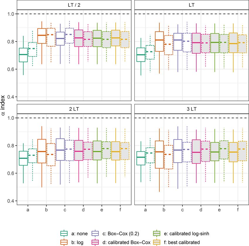
2020                                                      L. Berthet et al.: Uncertainty assessment when forecasting high flows

                                                                      2.1.2   Hydrological model

                                                                      We used discharge forecasts computed by the GRP rainfall–
                                                                      runoff model. The GRP model is designed for flood forecast-
                                                                      ing and is currently used by the FFS in France in operational
                                                                      conditions (Furusho et al., 2016; Viatgé et al., 2018). It is
                                                                      a deterministic lumped storage-type model that uses catch-
                                                                      ment areal rainfall and PE as inputs. In forecasting mode
                                                                      (Appendix A), the model also assimilates discharge obser-
                                                                      vations available when issuing a forecast to update the main
                                                                      state variable of the routing function and to update the out-
                                                                      put discharge. In this study, it is run at an hourly time step,
                                                                      and forecasts are issued for several lead times ranging from
                                                                      1 to 72 h. More details about the GRP model can be found in
                                                                      Appendix A.
                                                                         Since herein only the ability of the post-processor to ex-
                                                                      trapolate uncertainty quantification is studied, the model is
                                                                      fed only with observed rainfall (no forecast of precipitation),
                                                                      in order to reduce the impact of the input uncertainty. For the
                                                                      same reason, the model is calibrated in forecasting mode over
                                                                      the 10-year series by minimising the sum of squared errors
                                                                      for a lead time taken as the LT. The results will be presented
                                                                      for four lead times, – LT / 2, LT, 2 LT and 3 LT – to cover the
Figure 1. The set of 154 unregulated catchments used in this study.   different behaviours that can be seen when data assimilation
Average altitude is given in metres above sea level (m a.s.l.).       is used to reduce errors in an operational flood forecasting
                                                                      context (Berthet et al., 2009).

2     Data and methods                                                2.1.3   Empirical hydrological uncertainty
                                                                              processor (EHUP)
2.1     Data and forecasting model
                                                                      We used the empirical hydrological uncertainty proces-
2.1.1    Catchments and hydrological data                             sor (EHUP) presented in Bourgin et al. (2014). It is a data-
                                                                      based and non-parametric approach in order to estimate the
We used a set of 154 unregulated catchments spread through-           conditional predictive uncertainty distribution. This post-
out France (Fig. 1) over various hydrological regimes and             processor has been compared to other post-processors in ear-
forecasting contexts to provide robust answers to our re-             lier studies and proved to provide relevant results (Bourgin,
search questions (Andréassian et al., 2006; Gupta et al.,             2014). It is now used by operational FFS in France under
2014). They represent a large variability in climate, to-             the operational tool called OTAMIN (Viatgé et al., 2019).
pography and geology in France (Table 1), although their              The main difference with many other post-processors (such
hydrological regimes are little or not at all influenced by           as the MCP, the meta-Gaussian processor, the BJP or the
snow accumulation. Hourly rainfall, potential evapotranspi-           BFS) is that no assumption is made about the shape of the
ration (PE) and streamflow data series were available over the        uncertainty distribution, which brings more flexibility to rep-
1997–2006 period. PE was estimated using a temperature-               resent the various forecast error characteristics encountered
based formula (Oudin et al., 2005). Rainfall and temperature          in large-sample modelling. We will discuss the impact of this
data come from a radar-based reanalysis produced by Météo-            choice in Sect. 4.2.
France (Tabary et al., 2012). Discharge data were extracted              The basic idea of the EHUP is to estimate empirical quan-
from the national streamflow HYDRO archive (Leleu et al.,             tiles of errors stratified by different flow groups to account for
2014). When a hydrological model is used to issue forecasts,          the variation of the forecast error characteristics with fore-
it is often necessary to compare the lead time to a character-        cast magnitude. Since forecast error characteristics also vary
istic time of the catchment (Sect. 2.1.2). For each catchment,        with the lead time when data assimilation is used, the EHUP
the lag time (LT) is estimated as the lag time maximising the         is trained separately for each lead time.
cross-correlation between rainfall and discharge time series.

Hydrol. Earth Syst. Sci., 24, 2017–2041, 2020                                       www.hydrol-earth-syst-sci.net/24/2017/2020/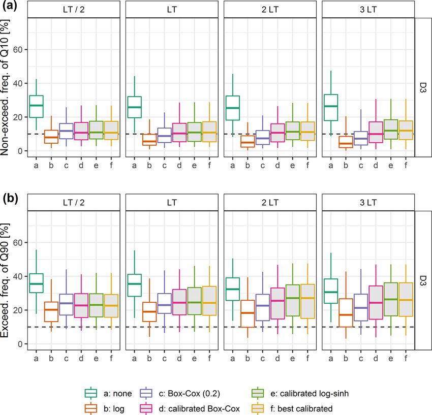
L. Berthet et al.: Uncertainty assessment when forecasting high flows                                                           2021

Table 1. Characteristics of the 154 catchments, computed over the 1997–2006 data series.

                                                                                             Quantiles
                                                                        0      0.05   0.25    0.50       0.75   0.95     1
               Catchment area (km2 )                                    9       27     79     184     399        942   3260
               Average altitude (m above sea level)                    64       92    188     376     589        897   1050
               Average slope (%)                                        2        3      6       9      18         32     39
               Lag time (h)                                             3        5      9      12      19         29     33
               Mean annual rainfall (mm yr−1 )                        639      727    876    1003    1230       1501   1841
               Mean annual potential evapotranspiration (mm yr−1 )    549      549    631     659     700        772    722
               Specific mean annual discharge (mm yr−1 )               53      142    262     394     583       1114   1663
               Mean annual discharge (m3 s−1 )                          1        1      1       2       5         17     53
               Maximum hourly rainfall (mm h−1 )                       10       12     16      20      26         41     61
               Quantile 0.99 of the hourly discharge (m3 s−1 )          1        2      6      15      33        115    296

  For each lead time separately, the following steps are used:            The EHUP can be applied after a preliminary data trans-
                                                                       formation, and by adding a final step to back-transform the
  1. Training:                                                         predictive distributions obtained in a transformed space. In
       – The flow groups are obtained by first ordering the            previous work, we used the log transformation because it
         forecast–observation pairs according to the fore-             ensures that no negative values are obtained when estimat-
         casted values and then stratifying the pairs into a           ing the predictive uncertainty for low flows (Bourgin et al.,
         chosen number of groups (in this study, we used               2014). When estimating the predictive uncertainty for high
         20 groups), so that each group contains the same              flows, the data transformation has a strong impact in extrap-
         number of pairs.                                              olation, because the variation of the extrapolated predictive
                                                                       distribution, which is constant in the transformed space, is
       – Within each flow group, errors are calculated as the          controlled in the real space by the behaviour of the inverse
         difference between the two values of each forecast–           transformation, as explained below.
         observation pair, and several empirical quantiles
         (we used 99 percentiles) are calculated in order to           2.1.4    The different transformation families
         characterise the distribution of the error values.
                                                                       Many uncertainty assessment methods mentioned in the In-
  2. Application:                                                      troduction use a variable transformation to handle the het-
       – The predictive uncertainty distribution that is asso-         eroscedasticity of the residuals and account for the varia-
         ciated with a given (deterministic) forecasted value          tion of the prediction distributions with the magnitude of the
         is defined by adding this forecasted value to the em-         predicted variable. Here, we briefly recall a number of vari-
         pirical quantiles that belong to the same flow group          able transformations commonly used in hydrological mod-
         as the forecasted value.                                      elling. Let y and ỹ be the observed and forecasted variables
                                                                       (here, the discharge), respectively, and ε = y − ỹ the residu-
   Since this study focuses on the extrapolation case, the val-        als. When using a transformation g, we consider the residuals
idation is achieved with deterministic forecasts higher than           ε 0 = g(y) − g(ỹ).
the highest one used for the calibration. Therefore, only the              Three analytical transformations are often met in hydro-
highest-flow group of the calibration data is used to esti-            logical studies: the log, Box–Cox and log–sinh transfor-
mate the uncertainty assessment (to be used on the control             mations. The log transformation is commonly used (e.g.
data). This highest-flow group contains the top 5 % pairs of           Morawietz et al., 2011):
the whole training data, ranked by forecasted values. This
threshold is chosen as a compromise between focusing on                g1 : y 7 −→ log(y + a),                                    (1)
the highest values and using a sufficiently large number of
forecast–observation pairs when estimating empirical quan-             where a is a small positive constant to deal with y val-
tiles of errors. In extrapolation, when the forecast discharge         ues close to 0. It can be taken as equal to 0 when focus-
is higher than the highest value of the training period, the           ing on large discharge values. This transformation has no
predictive distribution of the error is kept constant, i.e. the        parameter to be calibrated. Applying a statistical model to
same values of the empirical quantiles of errors are used, as          residuals computed on log-transformed variables may be
illustrated in Fig. 5.                                                 interpreted as using a corresponding model of multiplica-
                                                                       tive error (e.g. assuming a Gaussian model for residuals

www.hydrol-earth-syst-sci.net/24/2017/2020/                                           Hydrol. Earth Syst. Sci., 24, 2017–2041, 2020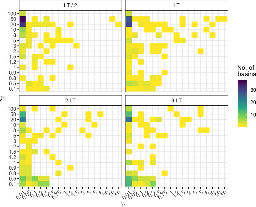
2022                                                       L. Berthet et al.: Uncertainty assessment when forecasting high flows

of log-transformed discharges is equivalent to a log-normal
model of the multiplicative errors y/ỹ). Therefore, it may be
adapted to strongly heteroscedastic behaviours. It has been
used successfully to assess hydrological uncertainty (Yang
et al., 2007b; Schoups and Vrugt, 2010; Bourgin et al., 2014).
   The Box–Cox transformation (Box and Cox, 1964) is a
classic transformation that is quite popular in the hydrologi-
cal community (e.g. Yang et al., 2007b; Wang et al., 2009;
Hemri et al., 2015; Reichert and Mieleitner, 2009; Singh
et al., 2013; Del Giudice et al., 2013):

                (y + a)λ − 1
g2[λ] : y 7−→                if λ 6 = 0 and g2[λ] = g1 if λ = 0.
                     λ
                                                                   (2)

Here a is taken as being equal to 0 (as for the log transforma-
tion); the Box–Cox transformation is then a one-parameter
transformation. It makes it possible to cover very differ-
                                                                         Figure 2. The inverse transformation explains the final effect on
ent behaviours. The log transformation is a special case of
                                                                         the uncertainty assessment: the constant probability distribution in
the Box–Cox transformation when the calibration results in               the transformed space (provided by the EHUP) will result in a dis-
λ = 0. In contrast, applying the Box–Cox transformation                  tribution in the untransformed space, whose evolution depends on
with λ = 1 to the variable y to model the distribution of                the behaviour of the inverse data transformation. Here, the Box–
their residuals is equivalent to applying no transformation              Cox transformation provides different behaviours, depending on its
(Fig. 2). McInerney et al. (2017) obtained their most reliable           parameter value (λ). It ranges from an affine transformation (equiv-
and sharpest results with λ = 0.2 over 17 perennial catch-               alent to no transformation; red dashed line) to the log transforma-
ments.                                                                   tion (thick green dashed line). With a single parameterisation, the
   More recently, the log–sinh transformation has been pro-              log–sinh transformation can be equivalent to the log transformation
posed (Wang et al., 2012; Pagano et al., 2013). It is a two-             for values of y much smaller than the value of its parameter β and
                                                                         equivalent to an affine transformation for large values of y (much
parameter transformation:
                                                                         higher than β; see Appendix B).

                                α+y
g3[α,β] : y 7 −→ β · log sinh             .                  (3)
                                 β
                                                                         tion, quantile by quantile. While several hydrological pro-
This transformation provides more flexibility. Indeed, for               cessors such as the HUP, MCP and QR encompass the NQT-
y  α and y  β, the log–sinh transformation reduces to no               transformed variables, Bogner et al. (2012) warn against
transformation, while for α  y  β it is equivalent to the              the drawbacks of this transformation, which is by construc-
log transformation (Fig. 2). Thus, with the same parameteri-             tion not suited for the extrapolation context and requires ad-
sation, it can result in very different behaviours depending on          ditional assumptions to model the tails of the distribution
the magnitude of the discharge. Applying no transformation               (Weerts et al., 2011; Coccia and Todini, 2011). This is why
may be intuitively attractive when modelling the distribution            we did not test this transformation in this study focused on
of residuals for large discharge values when the variance is             the extrapolation context.
no longer expected to increase (homoscedastic behaviour).
It is then particularly attractive when modelling predictive             2.2     Methodology: a testing framework designed for
uncertainty in an extrapolation context, in order to avoid an                    extrapolation context assessment
excessively “explosive” assessment of the predictive uncer-
tainty for large discharge values.                                       2.2.1    Testing framework
   In addition to the log transformation used by Bourgin et al.
(2014), in this study we tested the Box–Cox and the log–sinh             The EHUP is a non-parametric approach based on the char-
transformations to explore more flexible ways to deal with               acteristics of the distribution of residuals over a training data
the challenge of extrapolating prediction uncertainty distri-            set. Moreover, the Box–Cox and the log–sinh transforma-
butions (Fig. 2). The impacts of the data transformations used           tions are parametric and require a calibration step. There-
in this study are illustrated in Fig. 3.                                 fore, the methodology adopted for this study is a split-sample
   Another common variable transformation is the normal                  scheme test inspired by the differential split-sample scheme
quantile transformation (NQT; e.g. Kelly and Krzysztofow-                of Klemes̆ (1986) and based on three data subsets: a data
icz, 1997). It is a transformation without a calibrated param-           set for training the EHUP, a data set for calibrating the pa-
eter linking a given distribution and the Gaussian distribu-             rameters of the variable transformation and a control data set

Hydrol. Earth Syst. Sci., 24, 2017–2041, 2020                                           www.hydrol-earth-syst-sci.net/24/2017/2020/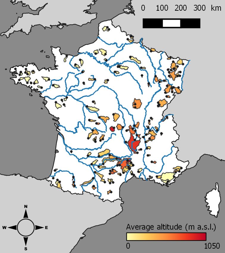
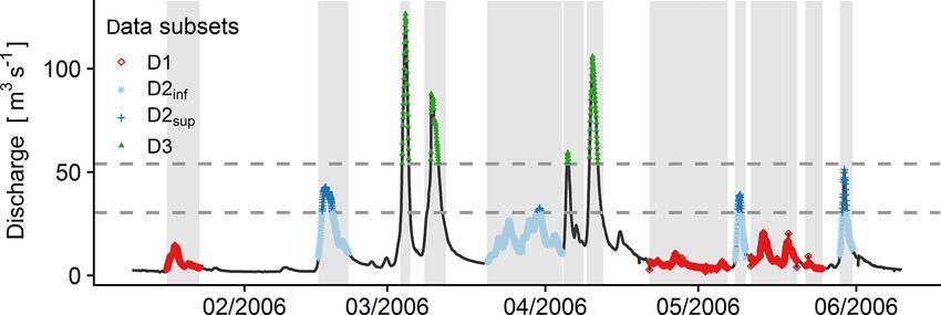
L. Berthet et al.: Uncertainty assessment when forecasting high flows                                                                     2023

Figure 3. Predictive 0.1 and 0.9 quantiles when assessed with no transformation, the log transformation, the Box–Cox transformation with
its λ parameter equal to 0.5 and the log–sinh transformation with its α and β parameters equal to 0.1 and 8, on the Ill River at Didenheim
(668 km2 ) for a lead time equal to LT, (a) as a function of the deterministic forecasted discharge and (b) for the flood event on 3 March 2006.
The heteroscedasticity strongly differs from one variable transformation to another.

for evaluating the predictive distributions when extrapolating            selection was made using the forecasted discharge and not
high flows.                                                               the observed discharge.

2.2.2   Events selection                                                  2.2.3    Selection of the data subsets

To populate the three data subsets with independent data,                 The selected events were then gathered into three events sets
separate flood events were first selected by an iterative proce-          – G1, G2 and G3 – based on the magnitude of their peaks and
dure similar to those detailed by Lobligeois et al. (2014) and            the number of useful time steps for each test phase (training
Ficchì et al. (2016): (1) the maximum forecasted discharge of             of the EHUP post-processor, calibration of the variable trans-
the whole time series was selected; (2) within a 20 d period              formations and evaluation of the predictive distributions):
before (after) the peak flow, the beginning (end) of the event            G1 contains the lowest events, while the highest events are
was placed at the preceding (following) time step closest to              in G3.
the peak at which the streamflow is lower than 20 % (25 %) of                The selection of the data subsets was tailored to study the
the peak flow value; and (3) the event was kept if there was              behaviour of the post-processing approach in an extrapola-
less than 10 % missing values, if the beginning and end of                tion context. The control data subset had to encompass only
the event were lower than 66 % of the peak flow value and if              time steps with simulated discharge values higher than those
the peak value was higher than the median value of the time               met during the training and calibration steps. Similarly, the
series. The process is then iterated over the remaining data              calibration data subset had to encompass time steps with sim-
to select all events. A minimum time lapse of 24 h was en-                ulated discharge values higher than those of the training sub-
forced between two events, ensuring that consecutive events               set.
are not overlapping and that the autocorrelation between the                 To achieve these goals, only the time steps within flood
time steps of two separate events remains limited.                        events were used. We distinguished four data subsets, as il-
   The number of events and their characteristics vary greatly            lustrated in Fig. 4. The subset D1 gathered all the time steps
among catchments, as summarised in Table 2. Note that the                 of the events of the G1 group. Then, the set D2 of the time
events selected for one catchment can slightly differ for the             steps of the events of the G2 group was split into two subsets:
four different lead times considered in this study, because the           D2sup gathered all the time steps with forecasted discharge

www.hydrol-earth-syst-sci.net/24/2017/2020/                                              Hydrol. Earth Syst. Sci., 24, 2017–2041, 2020
2024                                                       L. Berthet et al.: Uncertainty assessment when forecasting high flows

Table 2. Characteristics of the events selected for the lead time (LT) over the 1997–2006 data series.

                                                                                                   Quantiles
                                                                             0     0.05     0.25      0.50      0.75    0.95      1
         Total length of events (d)                                       663      1178     1299     1505       1808    2061    2762
         Number of events G1                                               28        65      114      141        193     276     434
         Number of events G2                                                8        16       23       32         43      58     170
         Number of events G3                                                7        12       19       26         35      46     162
         Specific median value of the peak discharges G1 (mm h−1 )      0.009     0.022    0.041    0.062      0.098   0.184   0.266
         Specific median value of the peak discharges G2 (mm h−1 )      0.026     0.064    0.140    0.217      0.342   0.706   1.042
         Specific median value of the peak discharges G3 (mm h−1 )      0.050     0.131    0.295    0.439      0.701   1.896   3.071

values higher than the maximum met in D1, and D2inf was                  the same magnitude as those of the training subset. There-
filled with the other time steps. Finally, D3 was similarly              fore, the calibration subset has to encompass events of a
filled with all the time steps of the G3 events with forecasted          larger magnitude (D2sup ). The parameter set obtaining the
discharge values higher than the maximum met in D2.                      best criterion value was selected. In the second step, the
    The discharge thresholds used to populate the D1, D2sup              EHUP was trained on the highest-flow group of D1, D2inf
and D3 subsets from the events belonging to the G1, G2 and               and D2sup combined and using the parameter set obtained
G3 groups were chosen to ensure a sufficient number of time              during the calibration step. Then, the predictive uncertainty
steps in every subset. We chose to set the minimum number                distribution was evaluated on the control data set D3. Train-
of time steps in D3 and D2sup to 720 as a compromise be-                 ing the EHUP on the highest-flow group of the union of D1,
tween having enough data to evaluate the methods and keep-               D2inf and D2sup allows the uncertainty assessment to be con-
ing the extrapolation range sufficiently large. We lowered this          trolled from small to large degrees of extrapolation (on D3).
limit to 500 for the top 5 % pairs of D1, since this subset was          Indeed if we had kept the training on D1 only, we would
only used to build the empirical distribution by estimating              have not been able to test small degrees of extrapolation on
the percentiles during the training step and not used for eval-          independent data for every catchment (see the discussion in
uating the quality of the uncertainty assessment.                        Sect. 3.3).

2.2.4   Calibration and evaluation steps                                 2.3     Performance criteria and calibration

                                                                         2.3.1    Probabilistic evaluation framework
Since there are only one parameter for the Box–Cox trans-
formation and two parameters for the log–sinh transforma-                Reliability was first assessed by a visual inspection of the
tion, a simple calibration approach of the transformation pa-            probability integral transform (PIT) diagrams (Laio and
rameters was chosen: the parameter space was explored by                 Tamea, 2007; Renard et al., 2010). Since this study was car-
testing several parameter set values. For the Box–Cox trans-             ried out over a large sample of catchments, two standard nu-
formation, 17 values for the λ parameter were tested: from 0             merical criteria were used to summarise the results: the α
to 1 with a step of 0.1 and with a refined mesh for the sub-             index, which is directly related to the PIT diagram (Renard
intervals 0–0.1 and 0.9–1. For the log–sinh transformation, a            et al., 2010), and the coverage rate of the 80 % predictive in-
grid of 200 (α, β) values was designed for each catchment                tervals (bounded by the 0.1 and 0.9 quantiles of the predictive
based on the maximum value of the forecasted discharge in                distributions), used by the French operational FFS (a perfect
the D2 subset, as explained in greater detail in Appendix B.             uncertainty assessment would reach a value of 0.8). The α
   Note that the hydrological model was calibrated over the              index is equal to 1 − 2 · A, where A is the area between the
whole set of data (1997–2006) to make the best use of the                PIT curve and the bisector, and its value ranges from 0 to 1
data set, since this study focuses on the effect of extrapolation        (perfect reliability).
on the predictive uncertainty assessment only.                              The overall quality of the probabilistic forecasts was eval-
   We used a two-step procedure, as illustrated in Fig. 5.               uated with the continuous rank probability score (CRPS;
The first step was to calibrate the parametric transforma-               Hersbach, 2000), which compares the predictive distribution
tions. For each transformation and for each parameter set,               to the observation:
the empirical residuals were computed over D1 and D2sup ,
                                                                                      +∞
where the EHUP was trained on the highest-flow group of D1                      1 XN Z                       2
(see Sect. 2.1.3) and the calibration criterion was computed             CRPS =          Fk (Q) − H Q − Qk,obs dQ,                     (4)
                                                                                N k=1
on D2sup . Indeed, the data transformations have almost no                                   0
impact on the uncertainty estimation by EHUP for events of

Hydrol. Earth Syst. Sci., 24, 2017–2041, 2020                                             www.hydrol-earth-syst-sci.net/24/2017/2020/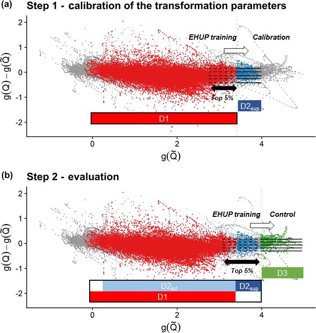
L. Berthet et al.: Uncertainty assessment when forecasting high flows                                                                2025

Figure 4. Illustration of the selection of the data subsets for the Ill River at Didenheim (668 km2 ). First, the events are selected (grey
highlighting). Then, the four data subsets are populated according to the thresholds (horizontal dashed lines). See Sect. 2.1.3 for more
details.

where N is the number of time steps, F (Q) is the predic-               However, in the authors’ experience, the latter is the control-
tive cumulative distribution, H the Heaviside function and              ling factor (Bourgin et al., 2014). Moreover, the CRPS val-
Qobs is the observed value. We used a skill score (CRPSS)               ues were often quite insensitive to the values of the log–sinh
to compare the mean CRPS to a reference, here the mean                  transformation parameters.
CRPS obtained from the unconditional climatology, i.e. from                In cases where an equal value of the α index was obtained,
the distribution of the observed discharges over the same data          we selected the parameter set that gave the best sharpness in-
subset. Values range from −∞ to 1 (perfect forecasts): a pos-           dex. For the log–sinh transformation, there were still a few
itive value indicates that the modelling is better than the cli-        cases where an equal value of the sharpness index was ob-
matology.                                                               tained, revealing the lack of sensitivity of the transformation
   For operational purposes, the sharpness of the probabilistic         in some areas of the parameter space. For those cases, we
forecasts was checked by measuring the mean width of the                chose to keep the parameter set that had the lowest α value
80 % predictive intervals. A dimensionless relative-sharpness           and the β value closest to max(Q).
                                                                                                         e
                                                                                                      D2
index was obtained by dividing the mean width by the mean
runoff:
     N
     P                                                                 3     Results
           q0.9 (Qk ) − q0.1 (Qk )
     k=1
1−                                    ,                        (5)      3.1    Results with the calibration data set D2sup
               N
               P
                    Qk,obs
              k=1                                                       Figure 6 shows the distributions of the α-index values ob-
where q90 (Q) and q10 (Q) are the upper and the lower bounds            tained with different transformations on the calibration data
of the 80 % predictive interval for each forecast, respectively.        set (D2sup ) for lead times LT / 2, LT, 2 LT and 3 LT. The dis-
The sharper the forecasts, the closer this index is to 1.               tributions are summarised with box plots. Clearly, not using
   In addition to the probabilistic criteria presented above,           any transformation leads to poorer reliability than any tested
the accuracy of the forecasts was assessed using the Nash–              transformation. In addition, we note that the calibrated trans-
Sutcliffe efficiency (NSE) calculated with the mean values              formations provide better results (although not perfect) than
of the predictive distributions (best value: 1).                        the uncalibrated ones in the calibration data set, as expected,
                                                                        and that no noticeable difference can be seen in Fig. 6 be-
2.3.2   The calibration criterion                                       tween the calibrated Box–Cox transformation (d), the cal-
                                                                        ibrated log–sinh transformation (e) and the best-calibrated
Since the calibration step aims at selecting the most reliable          transformation (f). Nevertheless, the uncalibrated log trans-
description of the residuals in extrapolation, the α index was          formation and Box–Cox transformation with parameter λ set
used to select the parameter set that yields the highest reli-          at 0.2 (BCλ=0.2 ) reach quite reliable forecasts. Comparing
ability for each catchment, each lead time and each trans-              the results obtained for the different lead times reveals that
formation. While other choices were possible, we followed               less reliable predictive distributions are obtained for longer
the paradigm presented by Gneiting et al. (2007): reliabil-             lead times, in particular for the transformations without a cal-
ity has to be ensured before sharpness. Note that the CRPS              ibrated parameter.
could have been chosen, since it can be decomposed as the                  Figures 7 and 8 show the distribution of parameter values
sum of two terms: reliability and sharpness (Hersbach, 2000).           obtained for the Box–Cox and the log–sinh transformation

www.hydrol-earth-syst-sci.net/24/2017/2020/                                             Hydrol. Earth Syst. Sci., 24, 2017–2041, 2020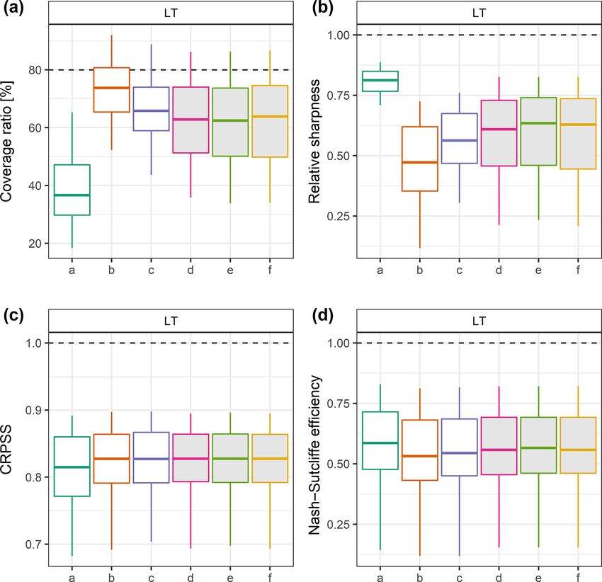
2026 L. Berthet et al.: Uncertainty assessment when forecasting high flows
Figure 5. Residuals as a function of the forecast discharges in the transformed space. The horizontal dashed lines represent the 0.1, 0.25,
0.5, 0.75 and 0.9 quantiles of the residuals computed during the training phase of the EHUP post-processor, for the highest-flow group
(top 5 % pairs of the training data ranked by forecasted values). The straight horizontal lines represent their use in assessing the predictive
uncertainty in extrapolation during (a) the calibration step of the variable transformation parameters and (b) the evaluation step of the
predictive uncertainty. During the calibration step (a), many parameters set values are tested, while only the calibrated set of transformation
parameters is used during the evaluation step (b). The vertical dashed lines show the beginning of the extrapolation range. The grey dots
are the data pairs which are not selected in D1, D2inf , D2sup or D3: they are not used during the calibration step or the evaluation step.
Illustration from the Ill River at Didenheim, 668 km2 . Data used for the EHUP training at each step is sketched by a thick rectangle. In this
study, only the top 5 % pairs of the training data ranked by forecasted values are used to estimate the residual distribution, since we focus on
the extrapolation behaviour of the EHUP.
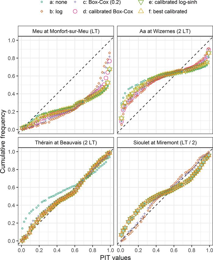
during the calibration step. The distributions vary with lead catchments and with lead time because of the strong impact
time. While the log transformation behaviour is frequently of data assimilation.
chosen for LT/2 and LT, the additive behaviour (correspond-
ing to the use of no transformation; see Sect. 2.1.4) becomes 3.2 Results with the D3 control data set
more frequent for 2 and 3 LT. A similar conclusion can be
drawn for the log–sinh transformation: a low value of α and 3.2.1 Reliability
a high value of β yield a multiplicative behaviour that is fre-
quently chosen, for all lead times, but less for 2 and 3 LT than First, we conducted a visual inspection of the PIT diagrams,
for LT/2 and LT. This explains in particular the loss of relia- which convey an evaluation of the overall reliability of the
bility that can be seen for the log transformation for 3 LT in probabilistic forecasts (examples in Fig. 9). In some cases,
Fig. 6. These results reveal that the extrapolation behaviour the forecasts are reliable (e.g. the Thérain River at Beauvais,
of the distributions of residuals is complex. It varies among 755 km2 , except if no transformation is used). Alternatively,
these diagrams may show quite different patterns, highlight-
Hydrol. Earth Syst. Sci., 24, 2017–2041, 2020 www.hydrol-earth-syst-sci.net/24/2017/2020/L. Berthet et al.: Uncertainty assessment when forecasting high flows 2027 Figure 6. Distributions of the α-index values on the calibration data set D2sup , obtained with different transformations for four lead times (the filled box plots represent the calibrated distributions). Box plots (5th, 25th, 50th, 75th and 95th percentiles) synthesise the variety of scores over the catchments of the data set. The optimal value is represented by the horizontal dashed lines. Figure 7. Distribution over the basins of the values of the Box–Cox transformation parameter obtained during the calibration step for the four different lead times. ing bias (e.g. the Meu River at Montfort-sur-Meu, 477 km2 ) and upper bounds of the predictive interval communicated or under-dispersion (e.g. the Aa River at Wizernes, 392 km2 , to the authorities, are of particular interest. The 80 % predic- or the Sioulet River at Miremont, 473 km2 ; for the latter, the tive interval (bounded by the 0.1 and 0.9 quantiles) is mostly calibration on D2sup leads to log–sinh and Box–Cox trans- used in France. It is expected that the non-exceedance fre- formations equivalent to no transformation, which turns out quency of the lower bound and the exceedance frequency of not to be relevant for the control data set, where the log and the upper bound remain close to 10 % for a reliable predic- the Box–Cox transformations are more reliable). tive distribution. Deviations from these frequencies indicate Then the distribution of the α-index values in Fig. 10 re- biases in the estimated quantiles. Figure 12 reveals that on veals a significant loss of reliability compared to the values average the 0.1 quantile is generally better assessed than the obtained with the calibration data set (Fig. 6). We note that 0.9 quantile on average, though the latter is generally more the log transformation is the most reliable approach for LT / 2 sought after for operational purposes. More importantly, the and is comparable to the Box–Cox transformation (BCλ=0.2 ) lack of reliability of the log transformation for the 3 LT lead for LT. With increasing lead time, the BCλ=0.2 transforma- time seen in Fig. 10 appears to be related to an underestima- tion becomes slightly better than the other transformations, tion of the 0.1 quantile, which is higher than for the other including the calibrated ones. In addition, comparing the re- tested transformations, while the 0.9 quantile is less under- sults obtained for the different lead times confirms that it is estimated than for the other transformations. These results challenging to produce reliable predictive distributions when highlight that reliability can have different complementary extrapolating at longer lead times. Overall, it means that the facets and that some parts of the predictive distributions can added value of the flexibility brought by the calibrated trans- be more or less reliable. In a context of flood forecasting, formations is not transferable in an independent extrapola- particular attention should be given to the upper part of the tion situation, as illustrated in Fig. 11. predictive distribution. In operational settings, non-exceedance frequencies of the quantiles of the predictive distribution, which are the lower www.hydrol-earth-syst-sci.net/24/2017/2020/ Hydrol. Earth Syst. Sci., 24, 2017–2041, 2020
2028                                                        L. Berthet et al.: Uncertainty assessment when forecasting high flows

Figure 8. Distribution over the basins of the values of the log–sinh transformation parameters obtained during the calibration step for the
four different lead times. γ1 = α/max(Q)
                                       e and γ2 = β/max(Q)   e (see Appendix B).
                                  D2                   D2

3.2.2    Other performance metrics                                      observed in an extrapolation context were correlated with
                                                                        some properties of the forecasts. First, Fig. 14 shows the re-
In addition to reliability, we looked at other qualities of             lationship between the α-index values obtained with D2sup
the probabilistic forecasts, namely the overall performance             and those obtained with D3 for three representative trans-
(measured by the CRPSS) and accuracy (measured by NSE).                 formations. The results indicate that it is not possible to an-
We also checked their sharpness (relative-sharpness metric).            ticipate the α-index values when extrapolating high flows in
The distributions of four performance criteria are shown for            D3 based on the α-index values obtained when extrapolating
LT in Fig. 13. We note that the log transformation has the              high flows in D2sup .
closest median value for the coverage ratio, at the expense                In addition, two indices were chosen to describe the de-
of a lower median relative-sharpness value, because of larger           gree of extrapolation: the ratio of the median of the fore-
predictive interval widths caused by the multiplicative be-             casted discharges in D3 over the median of the forecasted
haviour of the log transformation. In addition, the CRPSS               discharge in D2sup , and the ratio of the median of the fore-
and the NSE distributions have limited sensitivity to the               casted discharges in D3 over the discharge for a return pe-
variable transformation (also shown by Woldemeskel et al.               riod of 20 years (for catchments where the assessment of the
(2018) for the CRPS), even if we can see that not using                 vicennial discharge was available in the national database:
any transformation yields slightly better results. This con-            http://www.hydro.eaufrance.fr, last access: March 2020). In
firms that the CRPSS itself is not sufficient to evaluate the           both cases, no trend appears, regardless of the variable trans-
adequacy of uncertainty estimation. Similar results were ob-            formation used, with Spearman coefficients values (much)
tained for the other lead times (Supplement).                           lower than 0.33. The reliability can remain high for some
                                                                        catchments even when the magnitude of the events of the
3.3     Investigating the performance loss in an                        control data set is much higher than that of the training data
        extrapolation context                                           set (see Supplement for figures).
                                                                           Finally, we found no correlation with the relative accuracy
For operational forecasters, it is important to be able to pre-         of the deterministic forecasts either. The goodness of fit dur-
dict when they can trust the forecasts issued by their mod-             ing the calibration phase cannot be used as an indicator of
els and when their quality becomes questionable. Therefore
we investigated whether the reliability and reliability loss

Hydrol. Earth Syst. Sci., 24, 2017–2041, 2020                                          www.hydrol-earth-syst-sci.net/24/2017/2020/
L. Berthet et al.: Uncertainty assessment when forecasting high flows 2029
Figure 9. Examples of PIT diagrams obtained with the control data set D3, with different transformations at four locations.
the robustness of the uncertainty estimation in an extrapola- words, what is learnt during the calibration of the more com-
tion context (see Supplement for figures). plex parametric transformations does not yield better results
in an extrapolation context.
These results could be explained by the fact that the cal-
4 Discussion ibration did not result in the optimally relevant parameter
set. To investigate whether another calibration strategy could
4.1 Do more complex parametric transformations yield yield better results, we compared the performance on the
better results in an extrapolation context? control D3 data set when the calibration is achieved on the
D2sup data set (“f: best calibrated”) and on the D3 data set
Overall, the results obtained for the control data set suggest (“g: best reliability”). The results shown in Fig. 10 reveal
that the log transformation and the fixed Box–Cox transfor- that, even when the best parameter set is chosen among the
mation (BCλ=0.2 ) can yield relatively satisfactory α index 217 possibilities tested in this study (17 for the Box–Cox
and coverage ratio values given their multiplicative or near- transformation and 200 for the log–sinh transformation), the
multiplicative behaviour in extrapolation. More tapered be- α-index distributions are far from perfect and reliability de-
haviours that can be obtained with the calibrated Box–Cox creases with increasing lead time. This suggests that the sta-
or log–sinh transformations do not show advantages when bility of the distributions of residuals when extrapolating
extrapolating high flows on an independent data set. In other
www.hydrol-earth-syst-sci.net/24/2017/2020/ Hydrol. Earth Syst. Sci., 24, 2017–2041, 20202030 L. Berthet et al.: Uncertainty assessment when forecasting high flows
Figure 10. Distributions of the α-index values on the control data set D3, obtained with different transformations for four lead times (the
filled box plots represent the calibrated distributions). Box plots (5th, 25th, 50th, 75th and 95th percentiles) synthesise the variety of scores
over the catchments of the data set. The optimal values are represented by the horizontal dashed lines. Option “g” gives the best performance
that could be achieved with this model and this post-processor for these catchments (see the discussion in Sect. 4.1).
Figure 11. Scatter plots of the reliability α index obtained with the log transformation and the log–sinh transformation (a) in D2sup on the
calibration step and (b) on D3 in the control step.
high flows might be a greater issue than the choice of the vari- tion of a Gaussian distribution and use data transformations
able transformation. Nonetheless, the gap between the distri- to fulfil this hypothesis (Li et al., 2017). Examples are the
butions of the transformations without a calibrated parame- MCP or the meta-Gaussian model; the NQT was designed
ter (“b” and “c”), the best-calibrated transformation (“f”) and to precisely achieve it. In their study on autoregressive er-
the best performance that could be achieved (“g”) highlights ror models used as post-processors, Morawietz et al. (2011)
that it might be possible to obtain better results with a more showed that error models with an empirical distribution for
advanced calibration strategy. This is, however, beyond the the description of the standardised residuals perform bet-
scope of this study and is therefore left for further investiga- ter than those with a normal distribution. We first checked
tions. whether the variable transformation helped to reach a Gaus-
sian distribution of the residuals computed with the trans-
4.2 Empirically based versus distribution-based formed variables. Then we investigated whether better per-
approaches: does the distribution shape choice formance can be achieved using empirical transformed dis-
impact the uncertainty assessment in an tributions of residuals or using Gaussian distributions cali-
extrapolation context? brated on these empirical distributions.
We used the Shapiro–Francia test where the null hypoth-
Besides the reduction of heteroscedasticity, many studies use esis is that the data are normally distributed. For each para-
post-processors which are explicitly based on the assump- metric transformation, we selected the parameter set of the
Hydrol. Earth Syst. Sci., 24, 2017–2041, 2020 www.hydrol-earth-syst-sci.net/24/2017/2020/L. Berthet et al.: Uncertainty assessment when forecasting high flows 2031 Figure 12. Distributions over the catchment set of (a) the non-exceedance frequency of the 0.1 quantile and (b) the exceedance frequency of the 0.9 quantile on the control data set D3, obtained with the different transformations tested (the filled box plots are related to calibrated transformations). The optimal values are represented by the horizontal dashed lines. calibration grid which obtains the highest p value. For more from the use of the Gaussian distributions for all lead times. than 98 % of the catchments, the p value is lower than 0.018 In contrast, the predictive uncertainty assessment based on (0.023) when the Box–Cox transformation (the log–sinh the empirical distribution with the log transformation is more transformation) is used. This indicates that there are only a reliable than the one based on the Gaussian distribution. For few catchments for which the normality assumption is not short lead times, it is slightly better to use the empirical dis- to be rejected. In a nutshell, the variable transformations can tributions for the calibrated transformations (Box–Cox and stabilise the variance, but they do not necessarily ensure the log–sinh), but we observe a different behaviour for longer normality of the residuals. It is important not to overlook this lead times. For these longer lead times, assessing the pre- frequently encountered issue in hydrological studies. dictive uncertainty using the Gaussian distribution fitted to Even if there is no theoretical advantage to using the Gaus- the empirical distributions of transformed residuals obtained sian distribution calibrated on the transformed-variable resid- with the calibrated log–sinh or Box–Cox transformations is uals rather than the empirical distribution to assess the pre- the most reliable option. It is better than using the log trans- dictive uncertainty, we tested the impact of this choice. For formation with the empirical distribution, but not very differ- each transformation, the predictive uncertainty assessment ent from using the BCλ=0.2 transformation. obtained with the empirical transformed-variable distribu- Investigations on the impact of the choice between the em- tion of residuals is compared to the assessment based on the pirical and the Gaussian distributions on the post-processor Gaussian distribution whose mean and variance are those of performance are shown in the Supplement. They show that the empirical distribution. Figure 15 shows the α-index dis- the choice of the distribution is not the dominant factor. tributions obtained over the catchments for both options in the control data set D3. We note that no clear conclusion can be drawn. No transformation (or identity transformation), which does not reduce the heteroscedasticity at all, benefits www.hydrol-earth-syst-sci.net/24/2017/2020/ Hydrol. Earth Syst. Sci., 24, 2017–2041, 2020
You can also read