A mass-weighted isentropic coordinate for mapping chemical tracers and computing atmospheric inventories - Recent
←
→
Page content transcription
If your browser does not render page correctly, please read the page content below
Atmos. Chem. Phys., 21, 217–238, 2021
https://doi.org/10.5194/acp-21-217-2021
© Author(s) 2021. This work is distributed under
the Creative Commons Attribution 4.0 License.

A mass-weighted isentropic coordinate for mapping chemical
tracers and computing atmospheric inventories
Yuming Jin1 , Ralph F. Keeling1 , Eric J. Morgan1 , Eric Ray2 , Nicholas C. Parazoo3 , and Britton B. Stephens4
1 Scripps Institution of Oceanography, University of California San Diego, La Jolla, CA 92093, USA
2 National Oceanic and Atmospheric Administration, Boulder, CO 80305, USA
3 Jet Propulsion Laboratory, California Institute of Technology, Pasadena, CA 91109, USA
4 National Center for Atmospheric Research, Boulder, CO 80301, USA

Correspondence: Yuming Jin (y2jin@ucsd.edu)

Received: 13 August 2020 – Discussion started: 19 August 2020
Revised: 5 November 2020 – Accepted: 24 November 2020 – Published: 12 January 2021

Abstract. We introduce a transformed isentropic coordinate        1   Introduction
Mθe , defined as the dry air mass under a given equivalent
potential temperature surface (θe ) within a hemisphere. Like
θe , the coordinate Mθe follows the synoptic distortions of       The spatial and temporal distribution of long-lived chemical
the atmosphere but, unlike θe , has a nearly fixed relationship   tracers like CO2 , CH4 , and O2 / N2 typically includes regu-
with latitude and altitude over the seasonal cycle. Calcula-      lar seasonal cycles and gradients with latitude and pressure
tion of Mθe is straightforward from meteorological fields. Us-    (Conway and Tans, 1999; Ehhalt, 1978; Randerson et al.,
ing observations from the recent HIAPER Pole-to-Pole Ob-          1997; Rasmussen and Khalil, 1981; Tohjima et al., 2012).
servations (HIPPO) and Atmospheric Tomography Mission             These patterns are evident in climatological averages but are
(ATom) airborne campaigns, we map the CO2 seasonal cycle          potentially distorted on short timescales by synoptic weather
as a function of pressure and Mθe , where Mθe is thereby ef-      disturbances, especially at middle to high latitudes (i.e., pole-
fectively used as an alternative to latitude. We show that the    ward of 30◦ N and S) (Parazoo et al., 2008; Wang et al.,
CO2 seasonal cycles are more constant as a function of pres-      2007). With a temporally dense dataset such as from satellite
sure using Mθe as the horizontal coordinate compared to lat-      remote sensing or tower in situ measurements, climatological
itude. Furthermore, short-term variability in CO2 relative to     averages can be created by averaging over this variability. For
the mean seasonal cycle is also smaller when the data are or-     temporally sparse datasets such as from airborne campaigns,
ganized by Mθe and pressure than when organized by latitude       it may be necessary to correct for synoptic distortion.
and pressure. We also present a method using Mθe to com-             A common approach to correct synoptic distortion is to
pute mass-weighted averages of CO2 on a hemispheric scale.        use transformed coordinates rather than geographic coor-
Using this method with the same airborne data and applying        dinates (i.e., pressure–latitude), to take into account atmo-
corrections for limited coverage, we resolve the average CO2      spheric dynamics and transport barriers. Such coordinate
seasonal cycle in the Northern Hemisphere (mass-weighted          transformation has been used, for example, to reduce dynam-
tropospheric climatological average for 2009–2018), yield-        ically induced variability in the stratosphere using equiva-
ing an amplitude of 7.8 ± 0.14 ppm and a downward zero-           lent latitude rather than latitude as the horizontal coordinate
crossing on Julian day 173 ± 6.1 (i.e., late June). Mθe may be    (Butchart and Remsberg, 1986); to diagnose the tropopause
similarly useful for mapping the distribution and computing       profile using a tropopause-based rather than surface-based
inventories of any long-lived chemical tracer.                    vertical coordinate (Birner et al., 2002); to study the trans-
                                                                  port regime in the Arctic using a horizontal coordinate based
                                                                  on the polar dome (Bozem et al., 2019); and to study UTLS
                                                                  (upper troposphere–lower stratosphere) tracer data by using
                                                                  tropopause-based, jet-based, and equivalent latitude coordi-

Published by Copernicus Publications on behalf of the European Geosciences Union.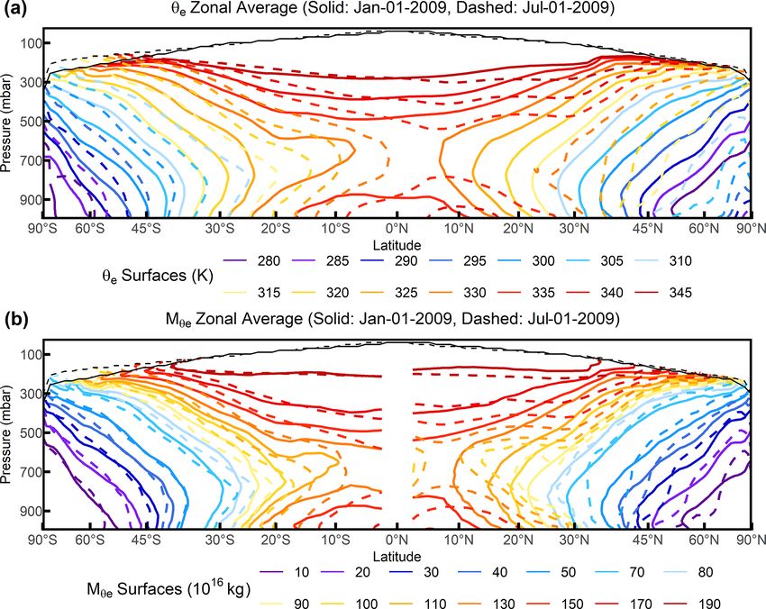
218                                                                      Y. Jin et al.: A mass-weighted isentropic coordinate

nates (Petropavlovskikh et al., 2019). In the troposphere, a      sphere with aircraft to compute the average of a chemical
transformed coordinate, the isentropic coordinate (θ), has        tracer within a large zonal domain.
been widely applied to evaluate the distribution of tracer data
(Miyazaki et al., 2008; Parazoo et al., 2011, 2012). As air
parcels move with synoptic disturbances, θ and the tracer         2     Methods
tend to be similarly displaced so that the θ –tracer relation-
ship is relatively conserved (Keppel-Aleks et al., 2011). Fur-    2.1    Meteorological reanalysis products
thermore, vertical mixing tends to be rapid on θ surfaces,
so θ and tracer contours are often nearly parallel (Barnes et     The calculation of Mθe requires the distribution of dry air
al., 2016). However, θ varies greatly with latitude and alti-     mass and θe . For these quantities, we alternately use three re-
tude over seasons due to changes in heating and cooling with      analysis products: ERA-Interim (Dee et al., 2011), NCEP2
solar insolation, which complicates the interpretation of θ –     (Kanamitsu et al., 2002), and Modern-Era Retrospective
tracer relationships on seasonal timescales.                      analysis for Research and Applications Version 2 (MERRA-
   During analysis of airborne data from the HIAPER Pole-         2) (Gelaro et al., 2017). All products have a 2.5◦ horizon-
to-Pole Observations (HIPPO) (Wofsy, 2011) and the Atmo-          tal resolution. NCEP2 has a daily resolution, and we aver-
spheric Tomography Mission (ATom) (Prather et al., 2018)          age 6-hourly ERA-Interim fields and 3-hourly MERRA-2
airborne campaigns, we have found it useful to transform          fields to yield daily fields. ERA-Interim has 32 vertical lev-
potential temperature into a mass-based unit, Mθ , which we       els from 1000 to 1 mbar, with approximately 20 to 27 lev-
define as the total mass of dry air under a given isentropic      els in the troposphere. NCEP2 has 17 vertical levels from
surface in the hemisphere. In contrast to θ , which has large     1000 to 10 mbar, with approximately 8 to 12 levels in the
seasonal variation, Mθ has a more stable relationship to lati-    troposphere. MERRA-2 has 42 vertical levels from 985 to
tude and altitude, while varying in parallel with θ on synoptic   0.01 mbar, with approximately 21 to 25 levels in the tropo-
scales. Also, for a tracer which is well-mixed on θ, a plot of    sphere.
this tracer versus Mθ can be directly integrated to yield the
                                                                  2.2    Equivalent potential temperature (θe ) and dry air
atmospheric inventory of the tracer, because Mθ directly cor-
                                                                         mass (M) of the atmospheric fields
responds to the mass of air. We note that a similar concept
to Mθe has been introduced in the stratosphere by Linz et         We compute θe (K) using the following expression:
al. (2016), in which M(θ) is defined as the mass above the
θ surface, to study the relationship between age of air and                            Rd
diabatic circulation of the stratosphere.                                  Lv (T )      P0 Cpd
                                                                  θe = T +         ·w ·                                       (1)
   Several choices need to be made in the definition of Mθ ,                Cpd         P
including defining boundary conditions (e.g., in altitude and
latitude) for mass integration and whether to use potential       from Stull (2012). T (K) is the temperature of air; w (kg of
temperature θ or equivalent potential temperature θe . Here,      water vapor per kg of air mass) is the water vapor mixing
for boundaries, we use the dynamical tropopause (based on         ratio; Rd (287.04 J kg−1 K−1 ) is the gas constant for air; Cpd
the potential vorticity unit, PVU) and the Equator, thus in-      (1005.7 J kg−1 K−1 ) is the specific heat of dry air at constant
tegrating the dry air mass of the troposphere in each hemi-       pressure; P0 (1013.25 mbar) is the reference pressure at the
sphere. We also focus on Mθ defined using equivalent po-          surface, and Lv (T ) is the latent heat of evaporation at tem-
tential temperature (θe ) to conserve moist static energy in      perature T . Lv (T ) is defined as 2406 kJ kg−1 at 40 ◦ C and
the presence of latent heating during vertical motion, which      2501 kJ kg−1 at 0 ◦ C and scales linearly with temperature.
improves alignment between mass transport and mixing es-             Following Bolton (1980), we compute the water vapor
pecially within storm tracks in mid-latitudes (Parazoo et al.,    mixing ratio (w) from relative humidity (RH; kg kg−1 ) pro-
2011; Pauluis et al., 2008, 2010). We call this tracer Mθe .      vided by the reanalysis products and the formula for the sat-
   In this paper we describe the method for calculating Mθe       uration mixing ratio of water vapor (Ps,v ; mbar) modified by
and discuss its variability on synoptic to seasonal scales. We    Wexler (1976).
also discuss the time variation in the θe –Mθe relationship                          17.67·T
within each hemisphere and explore the stability of Mθe and       Ps,v = 0.06122 · e T +243.5                                 (2)
the θe –Mθe relationship using different reanalysis products.                          Ps,v
To illustrate the application of Mθe , we map CO2 data from       w = RH · 0.622 ·                                            (3)
                                                                                    P − Ps,v
two recent airborne campaigns (HIPPO and ATom) on Mθe .
Further, we show how Mθe can be used to accurately compute        We compute the total air mass of each grid cell x at time t,
the average CO2 concentration over the entire troposphere         Mx (t), shown in Eq. (4), from the product of the pressure
of the Northern Hemisphere using measurements from the            range and surface area and divided by a latitude- and height-
same airborne campaigns. We examine the accuracy of this          dependent gravity constant provided by Arora et al. (2011).
method and propose an appropriate way to sample the atmo-         The surface area is computed by using latitude (8), longitude

Atmos. Chem. Phys., 21, 217–238, 2021                                                https://doi.org/10.5194/acp-21-217-2021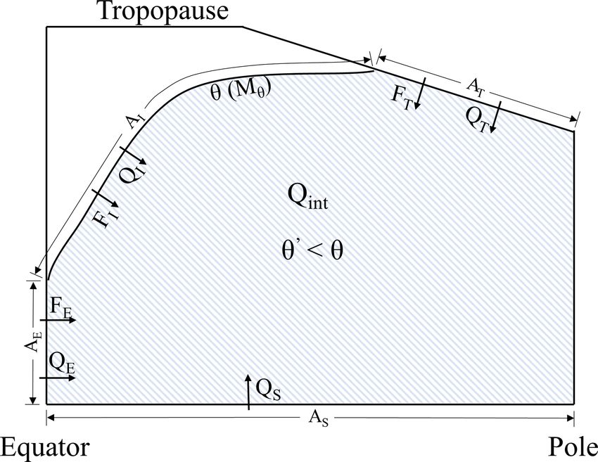
Y. Jin et al.: A mass-weighted isentropic coordinate 219
(λ), and the radius of the Earth (R, 6371 km). The total air 3 Characteristics of Mθe
mass of each grid cell is computed from
3.1 Spatial and temporal distribution of Mθe
1P
Mx = · |1 sin(8) · 1λ| · R 2 , (4)
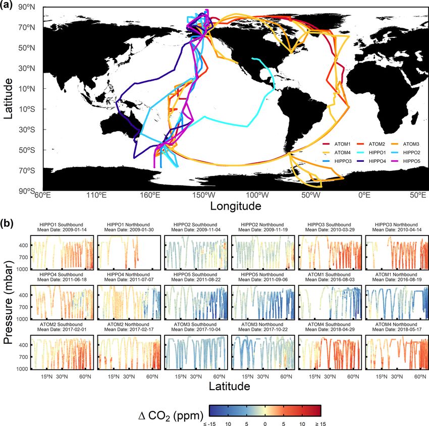
g Figure 2 shows snapshots of the distribution of zonal aver-
age θe and Mθe with latitude and pressure at two arbitrary
where 1 represents the difference between two boundaries
time slices (1 January 2009, 1 July 2009). Mθe is not con-
of each grid cell.
tinuous across the Equator because it is defined separately in
The gravity constant (g; kg m−2 ) is computed following
each hemisphere. By definition, each Mθe surface is exactly
Arora et al. (2011) as
aligned with a corresponding θe surface, and Mθe surfaces
have the same characteristics as θe surfaces, which decrease
g(8, h) = g0 · 1 + 0.0053 · sin2 (8)
with latitude and generally increase with altitude. Whereas
the zonal average θe surfaces vary by up to 20◦ in latitude
−0.000006 · sin2 (2 · 8) − 0.000003086 · h, (5)
over seasons, the meridional displacement of zonal average
Mθe is much smaller, with less than 5◦ in latitude poleward
where the reference gravity constant (g0 ) is assumed to be
of 30◦ N and S, as expected, because the zonal average dis-
9.78046 m s−2 and the height (h) in units of meters is com-
placement of atmospheric mass over seasons is small. This
puted from
small seasonal displacement is closely associated with the
h seasonality of vertical sloping of θe surfaces (Fig. 2). As the
P = P0 · e − H , (6)
mass under each Mθe surface is always constant, the change
where H is the scale height of the atmosphere and assumed in tilt must cause the meridional displacement. In the sum-
to be 8400 m. mer, the tilt is steeper (due to increased deep convection),
The dry air mass is then computed by subtracting the water so Mθe surfaces move poleward in the lower troposphere but
mass, computed from relative humidity, the saturation water move equatorward in the upper troposphere.
vapor mass mixing ratio, and the total air mass of the grid Mθe surfaces at given meridians (Fig. 3) in the North-
cell (Eq. 3). Since this study focuses on tracer distributions ern Hemisphere show clear zonal asymmetry, with larger
in the troposphere, we compute Mθe with an upper boundary and more complex displacements compared to the zonal
at the dynamical tropopause defined as the 2 PVU (potential averages, associated with differential heating by land and
vorticity units, 10−6 K kg−1 m2 s−1 ) surface. ocean and orographic stationary Rossby waves (Hoskins and
ERA-Interim and NCEP2 include hypothetical levels be- Karoly, 1981; Wills and Schneider, 2018). For example, over
low the true land or sea surface, for example, the 850 hPa the Northern Hemisphere ocean at 180◦ E (Fig. 3a) and from
level over the Himalaya, which we exclude in the calculation the summer to winter, Mθe surfaces move poleward in the
of Mθe . middle to high latitudes (e.g., poleward of 45◦ N) but move
equatorward in the mid- to low-latitude lower troposphere
2.3 Determination of Mθe (e.g., equatorward of 45◦ N, 900–700 mbar), with the magni-
tude smaller than 10◦ latitude in both. In comparison, over
We show a schematic of the conceptual basis for the calcu- the Northern Hemisphere land at 100◦ E (Fig. 3b) and from
lation of Mθe in Fig. 1. To compute Mθe , we sort all tropo- the summer to winter, Mθe surfaces move equatorward by
spheric grid cells in the hemisphere by increasing θe and sum up to 30◦ latitude, except in the high-latitude middle tropo-
the dry air mass over grid cells following sphere (e.g., poleward of 70◦ N, ∼ 500 mbar), where the flat
X Mθe surfaces lead to slightly poleward displacements. In the
Mθe (θe , t) = Mx (t)|θex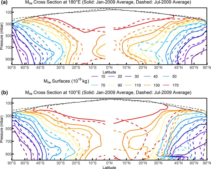
220                                                                             Y. Jin et al.: A mass-weighted isentropic coordinate

Figure 1. Schematic of the conceptual basis to calculate Mθe . Mθe of a given θe surface is computed by summing all dry air mass with a low
equivalent potential temperature in the troposphere of the hemisphere. This calculation yields a unique θe –Mθe relation at a given time point.

Figure 2. Snapshot of the distribution of (a) zonal average θe surfaces on 1 January 2009 (solid lines) and 1 July 2009 (dashed lines) and
(b) zonal average Mθe surfaces on 1 January 2009 (solid lines) and 1 July 2009 (dashed lines). The zonal average tropopause is also shown
here for 1 January 2009 (solid black line) and 1 July 2009 (dashed black line). θe , Mθe , and the tropopause are computed from ERA-Interim.

Northern Hemisphere summer are displaced poleward com-                    faces displace poleward in the lower troposphere but equa-
pared to the zonal average, consistent with a northward shift             torward in the upper troposphere. The displacements in the
of the intertropical convergence zone (ITCZ) over southern                lower troposphere (925 mbar) are greater in the Northern
Asia. The existence of these two branches may limit some                  Hemisphere, where the Mθe = 140 × 1016 kg surface, for ex-
applications of Mθe , as discussed in Sect. 4.                            ample, displaces poleward by 10◦ in latitude between winter
   Figure 4 shows the zonal average meridional displacement               and summer (Fig. 4b). Beside the seasonal variability, Fig. 4
of θe and Mθe with a daily resolution. In summer, Mθe sur-                also shows evident synoptic-scale variability.

Atmos. Chem. Phys., 21, 217–238, 2021                                                          https://doi.org/10.5194/acp-21-217-2021
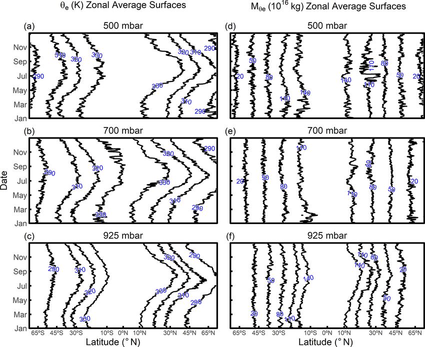
Y. Jin et al.: A mass-weighted isentropic coordinate                                                                                221

Figure 3. Mθe surfaces as January 2009 average (solid lines) and July 2009 average (dashed lines) for (a) 180◦ E (mostly over the Pacific
Ocean), and (b) 100◦ E (mostly over the Eurasia land in the Northern Hemisphere). Mθe and the tropopause are computed from ERA-Interim.

Figure 4. Time series of meridional displacement of selected zonal average θe (K) surfaces over a year at (a) 500 mbar, (b) 700 mbar, and
(c) 925 mbar. Meridional displacement of selected zonal average Mθe (1016 kg) surfaces over a year at (d) 500 mbar, (e) 700 mbar, and
(f) 925 mbar. The value of each surface is labeled. θe and Mθe are computed from ERA-Interim. Results shown are for the year 2009.

https://doi.org/10.5194/acp-21-217-2021                                                    Atmos. Chem. Phys., 21, 217–238, 2021
222                                                                           Y. Jin et al.: A mass-weighted isentropic coordinate

Figure 5. Snapshots (1 January 2009 and 1 July 2009) of the mass        Figure 6. Variability in Mθe of given θe surfaces (i.e., θe –Mθe look-
distribution of different Mθe bins from three pressure bins (surface    up table) over a year with a daily resolution in the Northern and
to 800 mbar, 800 to 500 mbar, and 500 mbar to tropopause). Mθe          Southern Hemisphere. Data from ERA-Interim are shown as a solid
is computed from ERA-Interim. Low Mθe bins are seen to have             line; MERRA-2 data are shown as a dashed line, and NCEP2 data
larger contributions from the air near the surface, and high Mθe bins   are shown as a dotted line. Results shown are for the year 2009.
have larger contributions from air aloft. Comparing the top and the
bottom panels shows that the seasonal differences in pressure con-
tributions are small except for the highest Mθe bins (160 × 1016 –      NCEP2 shows slightly larger deviations from ERA-Interim
180 × 1016 kg) and the lowest Mθe bin in the Northern Hemisphere        but by less than 8.5 × 10¹⁶ kg. The products are highly con-
(0–20 × 1016 kg).                                                       sistent in seasonal variability, and they also show agreement
                                                                        on synoptic timescales. The small difference between prod-
                                                                        ucts is expected because of different resolutions and methods
   Since the tilting of θe surfaces has an impact on the sea-           (Mooney et al., 2011). We expect these differences would be
sonal displacement of Mθe surfaces, the contribution of dif-            negligible for most applications of Mθe .
ferent pressure levels to the mass of a given Mθe bin must                 Figure 6 shows that, in both hemispheres, Mθe reaches its
also vary with season. In Fig. 5, we show these contribu-               minimum in summer and maximum in winter for a given
tions as two daily snapshots on 1 January and 1 July 2009.              θe surface, with the largest seasonality at the lowest θe (or
Low Mθe bins consist of air masses mostly below 500 mbar                Mθe ) values. The seasonality decreases as θe increases, fol-
near the pole. As Mθe increases, the contribution from the              lowing the reduction in the seasonality of shortwave absorp-
upper troposphere gradually increases while the contribution            tion at lower latitudes (Li and Leighton, 1993). The season-
from the surface to 800 mbar decreases to its minimum at                ality is smaller in the Southern Hemisphere, consistent with
around 100 × 1016 to 120 × 1016 kg. The contribution from               the larger ocean area and hence greater heat capacity and
the surface to 800 mbar increases as Mθe increases above                transport (Fasullo and Trenberth, 2008; Foltz and McPhaden,
120 × 1016 kg. The mass fraction shows only small varia-                2006). Figure 6 also shows that Mθe has significant synoptic-
tions with season, with the lower troposphere (surface to               scale variability although smaller than the seasonal variabil-
800 mbar) contributing slightly less in the low-Mθe bands and           ity. Synoptic variability is typically larger in winter than sum-
slightly more in the high-Mθe bands in the summer, which is             mer, as discussed below.
closely related to the seasonal tilting of corresponding θe sur-
faces.                                                                  3.3   Relationship to diabatic heating and mass fluxes

3.2   θe –Mθe relationship                                              A key step of the application of Mθe for interpreting tracer
                                                                        data is the generation of the look-up table that relates θe and
Figure 6 compares the temporal variation in Mθe of sev-                 Mθe . In this section, we address a tangential question of what
eral given θe surfaces (i.e., θe –Mθe look-up table) computed           controls the temporal variation in the look-up table, which is
from different reanalysis products for 2009. The deviations             not necessary for the application but may be of fundamental
are indistinguishable between ERA-Interim and MERRA-                    meteorological interest.
2, except near θe = 340 K, where MERRA-2 is systemati-                    As shown in Appendix A, the temporal variation in the
cally lower than ERA-Interim by 1.5 × 10¹⁶ to 6.5 × 10¹⁶ kg.            look-up table, Ṁθe = ∂t∂ Mθe (θe , t), can be related to underly-

Atmos. Chem. Phys., 21, 217–238, 2021                                                        https://doi.org/10.5194/acp-21-217-2021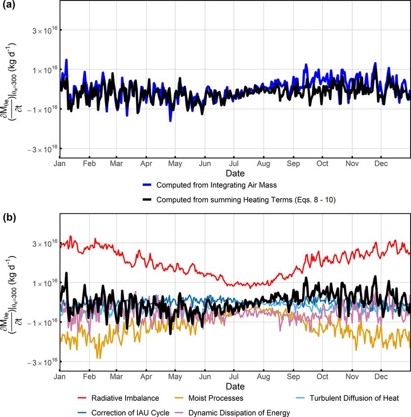
Y. Jin et al.: A mass-weighted isentropic coordinate                                                                                        223

ing mass and heat fluxes according to                                             table) with Mθe computed from the sum of the diabatic heat-
                                                                                  ing terms from MERRA-2 (via Eqs. 8 to 10). The compar-
            1 ∂Qdia (θe , t)                                                      ison focuses on the θe = 300 K surface, which does not in-
Ṁθe = −                     + mT (θe , t) + mE (θe , t) ,                (8)
           Cpd   ∂θe                                                              tersect with the Equator or tropopause, so the two mass flux
                                                                                  terms (mT , mE ) vanish. These two methods have a high cor-
where ∂Qdia  (θe ,t)
            ∂θe      (J s−1 K−1 ) is the effective diabatic heat-                 relation at 0.71. We do not expect perfect agreement because
ing, integrated over the full θe surface per unit width in θe ;                   Ṁθe computed by the sum of heating neglects turbulent wa-
mT (θe t) (kg s−1 ) is the net mass flux across the tropopause;                   ter vapor transport (QH2 O ), and only approximates Qevap as
and mE (θe t) (kg s−1 ) is the net mass flux across the Equator,                  discussed above. This relatively good agreement nevertheless
including all air with equivalent potential temperature of less                   demonstrates that the formulation based on MERRA-2 heat-
than θe . Qdia has contributions from internal heating with-                      ing terms includes the dominant processes that drive tem-
out ice formation (Q0int ), heating from ice formation (Qice ),                   poral variations in the look-up table. Figure 7a shows poorer
sensible heating from the surface (Qsen ), surface evapora-                       agreement from late August to October, which we also find in
tion (Qevap ), turbulent diffusion of heat (Qdiff ), and turbulent                other years (Figs. S1 and S2 in the Supplement) and on lower
transport of water vapor (QH2 O ) following                                       (e.g., θe = 290 K, Fig. S3) but not higher (e.g., θe = 310 K,
                                                                                  Fig. S4) surfaces, where the two methods agree better. The
Qdia (θe , t) = Q0int (θe , t) + Qice (θe , t) + Qsen (θe , t)
                                                                                  poor agreement may reflect a partial breakdown of the as-
             + Qevap (θe , t) + Qdiff (θe , t) + QH2 O (θe , t) . (9)             sumption that Qmst approximates the sum of Qice and Qevap ,
                                                                                  but further analysis is beyond the scope of this study.
The terms Qevap and QH2 O are expressed as heating rates
                                                                                     Figure 7b further breaks down the sum of the heating terms
by multiplying the underlying water fluxes by Lv (T )/Cpd .
                                                                                  in Eqs. (8) and (10) from MERRA-2 into individual com-
In order to quantify the dominant processes contributing to
                                                                                  ponents. Each term clearly displays variability on synoptic
temporal variation in Mθe , the terms in Eqs. (8) and (9) must
                                                                                  to seasonal scales. To quantify the contribution of different
be linked to diagnostic variables available in the reanaly-
                                                                                  terms on the different timescales, we separate each term into
sis or model products. Although there was no perfect match
                                                                                  a seasonal and synoptic component, where the seasonal com-
with any of the three reanalysis products, MERRA-2 pro-
                                                                                  ponent is derived by a two-harmonic fit with a constant offset
vides temperature tendencies for individual processes, which
                                                                                  and the synoptic component is the residual. We estimate the
can be converted to heating rates per Eq. 9 following
                                                                                  fractional contribution of each heating term on seasonal and
∂Qi (θe , t)   Cpd X dT
                                                                                synoptic timescales separately in Table 2, using the method
             =                    Mx ,                    (10)                    in Sect. S1 in the Supplement. On the seasonal timescale,
    ∂θe        1θe x     dt x,i
                                                                                  the variance is dominated by radiative heating and cooling of

                                                                     dT
                                                                                 the atmosphere and moist processes (including both ice for-
where i refers to a specific process (Q0int , Qice , etc.),          dt           mation and extra water vapor from surface evaporation) to-
                                                                              x
(K s−1 ) is the temperature tendency of grid cell x, Mx (kg) is                   gether, with prominent counteraction between them. On the
the mass of grid cell x, and 1θe is the width of the θe surface.                  synoptic timescale, dissipation of the kinetic energy of tur-
   There are five heating terms provided in the MERRA-                            bulence dominates the variance.
2 product, which we can approximately relate to terms in                             Similar analyses on different θe surfaces and in different
Eq. (9), as shown in Table 1. The first three terms (Qrad ,                       years (Figs. S1 to S4) all show that a combination of radia-
Qdyn , and Qana ) can be summed to yield Q0int ; the fourth                       tive heating and moist processes dominates the temporal vari-
(Qtrb ) is equal to the sum of Qdiff and Qsen ; and the fifth                     ation in Mθe on the seasonal timescale, while dissipation of
(Qmst ) approximates the sum of Qice and Qevap . MERRA-                           the kinetic energy of turbulence dominates on the synoptic
2 does not provide terms corresponding to QH2 O or Qevap ,                        timescale.
but Qmst represents heating due to moist processes, which
includes Qice plus water vapor evaporation and condensa-
tion within the atmosphere. This water vapor evaporation and                      4   Applications of Mθe as an atmospheric coordinate
condensation should be approximately equal to Qevap with
a small time lag when integrated over a θe surface because                        To illustrate the potential application of Mθe for interpret-
mixing is preferentially along θe surfaces and water vapor                        ing sparse data, we focus on the seasonal cycle of CO2 in
released into a θe surface by surface evaporation will tend to                    the Northern Hemisphere as resolved by two series of global
transport and precipitate from the same θe surface within a                       airborne campaigns, HIPPO and ATom. HIPPO consisted of
short time period (Bailey et al., 2019). Thus, the MERRA-2                        five campaigns between 2009 and 2011, and ATom consisted
term for heating by moist processes (Qmst ) should approxi-                       of four campaigns between 2016 and 2018. Each campaign
mate Qice + Qevap .                                                               covered from ∼ 150 to ∼ 14 000 m and from nearly pole to
   Figure 7a compares the temporal variation in Ṁθe com-                         pole, along both northbound and southbound transects. On
puted by integrating the dry air mass (i.e., θe –Mθe look-up                      HIPPO, both transects were over the Pacific Ocean, while

https://doi.org/10.5194/acp-21-217-2021                                                              Atmos. Chem. Phys., 21, 217–238, 2021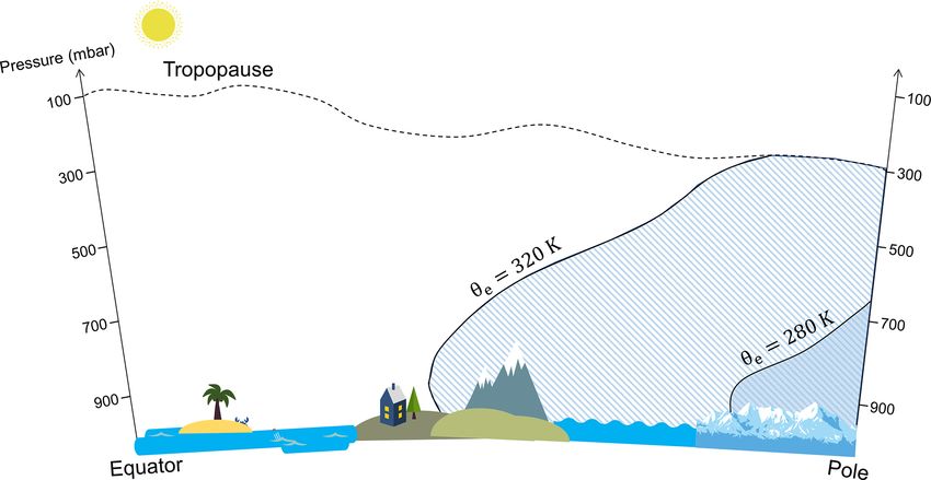
224                                                                            Y. Jin et al.: A mass-weighted isentropic coordinate

Table 1. Correspondence of heating variables between our derivation (Eq. 9) and MERRA-2.

                       Diabatic heating terms in    Diabatic heating terms in MERRA-2, ∂Q∂θ
                                                                                         i (θe ,t)
                                                                                                e
                       our derivation (Eq. 9)
                       Q0int                        1. Radiative heating (i.e., sum of shortwave and longwave ra-
                                                    diative heating, Qrad )
                                                    +
                                                    2. Absorption of kinetic energy that breaking the eddies (Qdyn )
                                                    +
                                                    3. The analysis tendency introduced during the corrector seg-
                                                    ment of the incremental analysis update (IAU) cycle (Qana )
                       Qdiff + Qsen                 4. Turbulent heat flux including surface sensible heating (Qtrb )
                       Qevap + Qice                 5. Moist processes including all latent heating due to conden-
                                                    sation and evaporation as well as to the mixing by convective
                                                    parameterization (Qmst )
                       QH2 O                        Not available

Figure 7. (a) Temporal variation in Mθe in the Northern Hemisphere at θe = 300 K computed by integrating air mass (blue line) and estimated
from the sum of five heating terms (Table 1) in MERRA-2 (black line). (b) The heating variables are decomposed into five contributions as
indicated (see Table 1). Results shown are for the year 2009.

Atmos. Chem. Phys., 21, 217–238, 2021                                                        https://doi.org/10.5194/acp-21-217-2021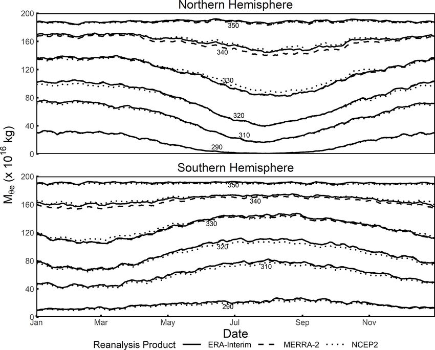
Y. Jin et al.: A mass-weighted isentropic coordinate                                                                                  225

Table 2. Fractional contribution of the individual heating terms in       terms with linear gain to the MLO record. Mθe is computed
Fig. 7b to their sum for θe = 300 K. The analysis is done separately      from ERA-Interim in this section.
on synoptic and seasonal components. The seasonal component is
based on a two-harmonic fit, and the synoptic component is defined        4.1   Mapping Northern Hemisphere CO2
as the residual. The fractional contributions sum to 1, while a pos-
itive contribution means in phase and negative contribution means
                                                                          A conventional method to display seasonal variations in CO2
anti-phase. A contribution of an absolute value that is bigger than 1
illustrates that the variability in the heating term is larger than the
                                                                          from airborne data is to plot time series of the data at a given
variability in the sum on the corresponding timescale.                    location or latitude and different pressure levels (Graven et
                                                                          al., 2013; Sweeney et al., 2015). In Fig. 9, we compare this
                Heating      Seasonal        Synoptic                     method using HIPPO and ATom airborne data, binning and
                terms      component       component                      averaging the data from each airborne campaign transect by
                                                                          pressure and latitude bins, with our new method, binning the
                Qrad             2.25             0.03                    data by pressure and Mθe . For each latitude bin, we choose
                Qmst            −1.39             0.07
                                                                          a corresponding Mθe bin which has approximately the same
                Qdyn             0.24             0.72
                                                                          meridional coverage in the lower troposphere. We remind the
                Qdyn             0.21             0.11
                Qana            −0.31             0.07                    reader that Mθe decreases poleward while also generally in-
                Sum                 1                1                    creasing with altitude (Figs. 2 to 4).
                                                                             As shown in Fig. 9, the transect averages of detrended
                                                                          CO2 (shown as points) from both binning methods resolve
                                                                          well-defined seasonal cycles (based on two-harmonic fit) in
                                                                          all bins, with higher amplitudes near the surface (low pres-
on ATom, southbound transects were over the Pacific Ocean                 sure) and at high latitudes (low Mθe ). However, binning by
and northbound transects were over the Atlantic Ocean. The                Mθe leads to much smaller variations in the mean seasonal
flight tracks are shown in Fig. 8a. We aggregate data from                cycle (shown as solid curves) with pressure, as expected, be-
each campaign into northbound and southbound transects                    cause moist isentropes are preferential surfaces for mixing.
within each hemisphere but only use data from the Northern                Also, within individual pressure bins, the short-term vari-
Hemisphere. We only consider tropospheric observations by                 ability relative to the mean cycles based on the distribution
excluding measurements from the stratosphere, which is de-                of all detrended observations (not shown as points but de-
fined by observed water vapor of less than 50 ppm and either              noted as 1σ values in Fig. 9) is smaller when binning by
O3 greater than 150 ppb or detrended N2 O to the reference                Mθe (F test, p < 0.01), except in the lower troposphere of
year of 2009 of less than 319 ppb. Water vapor and O3 were                the highest Mθe bin (90 × 1016 –110 × 1016 kg). The smaller
measured by the NOAA UCATS (Unmanned Aerial Sys-                          short-term variability is expected because Mθe tracks the syn-
tems Chromatograph for Atmospheric Trace Species; Hurst,                  optic variability in the atmosphere. When binning by lati-
2011) instrument and were interpolated to a 10 s resolution.              tude, the smallest short-term variability is found at the low-
N2 O was measured by the Harvard QCLS (Quantum Cas-                       est bin (surface–800 mbar) and the largest short-term vari-
cade Laser System; Santoni et al., 2014) instrument. Fur-                 ability is found in the highest bin (500 mbar tropopause), ex-
thermore, we exclude all near-surface observations within                 cept the highest latitude bin (45–55◦ N). When binning by
∼ 100 s of takeoffs and within ∼ 600 s of landings as well as             Mθe , in contrast, the short-term variability in the middle pres-
missed approaches, which usually show high CO2 variability                sure bin is always smaller than the higher and lower pres-
due to strong local influences. In situ measurements of CO2               sure bins (F test, p < 0.01), except for the 50-to-70 Mθe bin,
were made by three different instruments on both HIPPO                    where the difference between the lowest and middle pres-
and Atom. Of these, we use the CO2 measurements made by                   sure bins is not significant (based on 1σ levels). The lower
the NCAR Airborne Oxygen Instrument (AO2) with a 2.5 s                    variability in the middle troposphere may reflect the sup-
measurement interval (Stephens et al., 2020), for consistency             pression of variability from synoptic disturbances, leaving a
with planned future applications of APO (atmospheric poten-               clearer signal of the influence of surface fluxes of CO2 and
tial oxygen) computed from AO2. The differences between                   stratosphere–troposphere exchanges. We compare the vari-
instruments are small for our application (Santoni et al.,                ance of detrended airborne observations within each Mθe –
2014). The data used in this study are averaged to a 10 s res-            pressure bin with its fitted value. The fitted seasonal cycle of
olution, and we show the detrended CO2 values along each                  each bin explains 63.2 % to 90.5 % of the variability for dif-
airborne campaign transect for the Northern Hemisphere in                 ferent bins, with higher fractions in the middle troposphere.
Fig. 8b. Since we focus on the seasonal cycle of CO2 , all                   Figure 9 also shows the CO2 seasonal cycle at MLO,
airborne observations are detrended by subtracting an inter-              which falls within a single Mθe –pressure bin (90 × 1016 –
annual trend fitted to CO2 measured at the Mauna Loa Ob-                  110 × 1016 kg, 500–800 mbar) at all seasons. Although the
servatory (MLO) by the Scripps CO2 Program. This trend is                 airborne data in this bin span a wide range of latitudes (∼ 10–
computed by a stiff cubic spline function plus four-harmonic              75◦ N), the seasonal cycle averaged over this bin is very sim-

https://doi.org/10.5194/acp-21-217-2021                                                       Atmos. Chem. Phys., 21, 217–238, 2021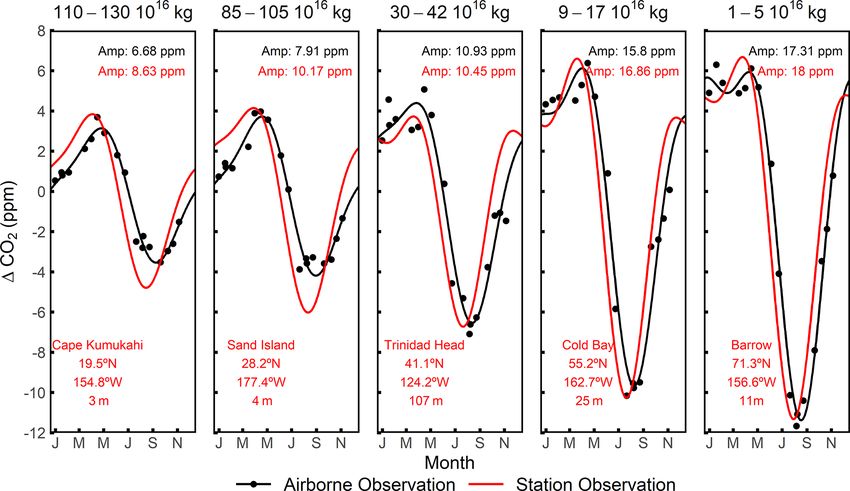
226                                                                            Y. Jin et al.: A mass-weighted isentropic coordinate

Figure 8. (a) HIPPO and ATom horizontal flight tracks colored by campaigns. (b) Latitude and pressure cross section of detrended CO2 of
each airborne campaign transect. CO2 is detrended by subtracting the MLO stiff cubic spline trend, which is computed by a stiff cubic spline
function plus four-harmonic functions with linear gain to the MLO record.

ilar to the cycle at MLO (airborne cycle leads by ∼ 10 d with           on the latitude of the station. To maximize sampling cover-
1.0 % lower amplitude). This small difference is within the             age, we bin the airborne data only by Mθe without pressure
1σ uncertainty in our estimation from airborne observation,             sub-bins. For mid- and high-latitude surface stations (right
and some difference is expected, since we choose a Mθe –                three panels), the seasonal amplitude of station CO2 and cor-
pressure bin wider than the seasonal variation in Mθe and               responding airborne CO2 are close (within 4 %–5 %), while
pressure at MLO.                                                        airborne cycles lag by 2–3 weeks. The lag presumably rep-
   It is also of interest to examine how CO2 data from surface          resents the slow mixing from the mid-latitude surface to the
stations fit into the framework based on Mθe . Figure 10 com-           high-latitude mid-troposphere (Jacob, 1999). In contrast, for
pares the CO2 seasonal cycle of five NOAA surface stations              low-latitude stations (left two panels) which generally sam-
(Cooperative Global Atmospheric Data Integration Project,               ple trade winds, the seasonal cycles differ significantly, in-
2019) with the cycle from the airborne observations binned              dicating that the air sampled at these stations is not rapidly
into selected Mθe bins. These surface stations are chosen to            mixed along surfaces of constant Mθe or θe with air aloft. As
be representative of different Mθe ranges. For the compar-              mentioned above (Sect. 3.1), surfaces of high Mθe within the
ison, we chose Mθe bins that span the seasonal maximum                  Hadley circulation have two branches, one near the surface
and minimum Mθe value of the station. These bins are nar-               and one aloft. A timescale of several months for transport
rower than the bins used in Fig. 9, in order to sharply focus           from the lower to the upper branch can be estimated from

Atmos. Chem. Phys., 21, 217–238, 2021                                                        https://doi.org/10.5194/acp-21-217-2021
Y. Jin et al.: A mass-weighted isentropic coordinate 227
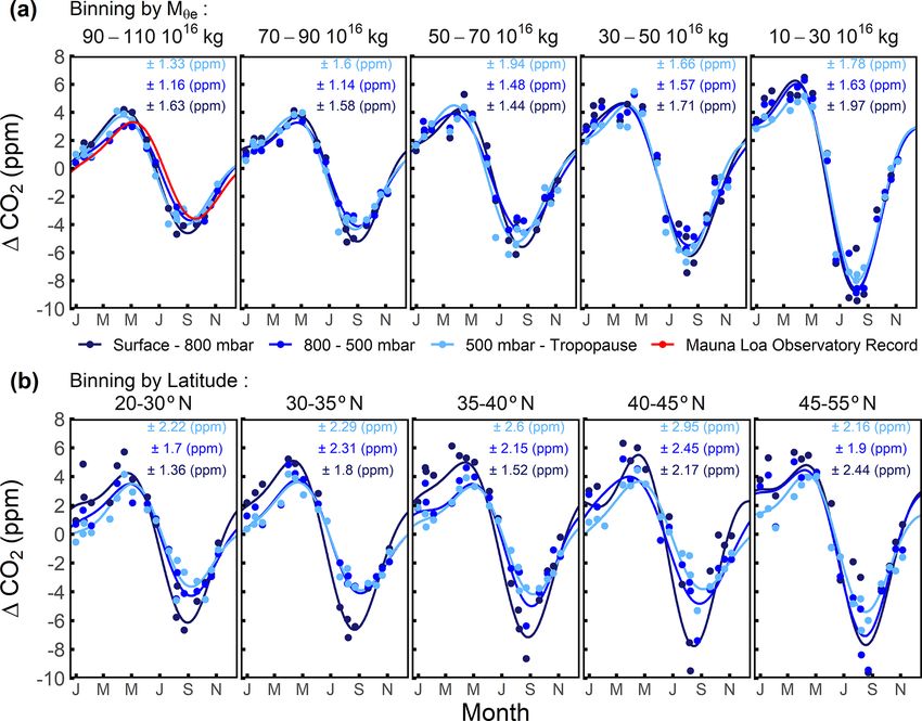
Figure 9. Seasonal cycles of airborne Northern Hemisphere CO2 data sorted by (a) Mθe –pressure bins and (b) latitude–pressure bins. Mθe
bins (1016 kg) and latitude bins are shown at the top of each panel. Pressure bins are colored. The latitude bounds are chosen to approximate
the meridional coverage of each corresponding Mθe bin in the lower troposphere. The seasonal cycle at MLO from 2009 to 2018 is shown in
the 90–110 Mθe bin panel, which spans the Mθe of the station. Airborne observations are first grouped into Mθe –pressure or latitude–pressure
bins and then averaged for each airborne campaign transect, shown as points. We filter out the points averaged from fewer than twenty 10 s
observations. The seasonal cycle of airborne data and MLO (2009–2018) are computed by a two-harmonic fit to the detrended time series.
The 1σ variability about the seasonal cycle fits for each Mθe –pressure or latitude–pressure bin is labeled at the top of each panel. These 1σ
values are based on the distribution of all binned observations (not shown), rather than on the distribution of average CO2 of each bin and
airborne campaign transect (shown).
the known overturning flows based on air mass flux stream 40◦ N. We use the θe –Mθe look-up table of the corresponding
functions (Dima and Wallace, 2003). This delay, plus strong date to assign a value of Mθe to each observation based on
mixing and diabatic effects (Miyazaki et al., 2008), ensures its θe . The observations for each transect are then sorted by
that the lower and upper branches are not well connected Mθe . The hemispheric average CO2 is calculated by trape-
on seasonal timescales. Our results nevertheless demonstrate zoidal integration of CO2 as a function of Mθe and divided
that the Mθe framework combining airborne and surface data by the total dry air mass as computed from the correspond-
could help understanding of details of atmospheric transport ing range of Mθe .
both along and across θe surfaces. To illustrate the Mθe integration method, we choose
HIPPO-1 Southbound and show CO2 measurements and
4.2 Computing the hemispheric mass-weighted average 1CO2 atmospheric inventory (Pg) as a function of Mθe
CO2 mole fraction in Fig. 11. The Northern Hemisphere tropospheric average
detrended 1CO2 is computed by integrating the area un-
der the curve (subtracting negative contributions) and divid-
We next illustrate the use of Mθe for computing the mass-
ing by the maximum value of Mθe within the hemisphere
weighted average of a long-lived chemical tracer by per-
(here 195.13 × 10¹⁶ kg). This yields a mass-weighted aver-
forming this exercise for CO2 in the Northern Hemisphere.
age detrended 1CO2 of 1.13 ppm for the full troposphere
We calculate the Northern Hemisphere tropospheric mass-
of the Northern Hemisphere. The trapezoidal integration has
weighted average CO2 from each airborne transect using a
a high accuracy because the data are dense over Mθe . The
method that assumes that CO2 is uniformly mixed on θe sur-
1CO2 atmospheric inventory is dominated by the domain
faces throughout the hemisphere (Barnes et al., 2016; Para-
Mθe < 120 ×1016 kg (mid-latitude to high latitude), which
zoo et al., 2011, 2012). We exclude airborne observation
has a large CO2 seasonal cycle driven by a temperate and
from HIPPO-1 Northbound due to the lack of data north of
https://doi.org/10.5194/acp-21-217-2021 Atmos. Chem. Phys., 21, 217–238, 2021228 Y. Jin et al.: A mass-weighted isentropic coordinate
Figure 10. CO2 seasonal cycles of multiple surface stations (2009–2018) compared to seasonal cycles of airborne observations averaged
over corresponding Mθe bin. The choice of Mθe bin is to approximate the range of Mθe at each corresponding surface station and is shown
at the top of each panel. Daily Mθe of the station is computed from ERA-Interim, based on its location. We detrend station and airborne
observations by subtracting the MLO stiff cubic spline trend. We compute average detrended CO2 for each airborne campaign transect and
each Mθe bin, shown as black points. The seasonal cycles are computed from a two-harmonic fit, with the seasonal amplitude (Amp) shown
in the upper right of each panel.
boreal ecosystem, with less than 4.1 % contributed by the ad-
ditional ∼ 38.8 % of the air mass outside this domain in the
low latitudes or upper troposphere (Fig. 11b), where 1CO2
differs less from the subtracted baseline.
We compute Northern Hemisphere mass-weighted aver-
age detrended 1CO2 for each airborne campaign transect
and fit the time series to a two-harmonic fit to estimate the
seasonal cycle (Fig. 12). We find that the cycle has a seasonal
amplitude of 7.9 ppm and a downward zero-crossing on Ju-
lian day 179, where the latter is defined as the date when the
detrended seasonal cycle changes from positive to negative.
To address the error in our estimation of the North-
ern Hemisphere mass-weighted average CO2 seasonal cy-
cle from HIPPO and Atom airborne observation, we con-
sider two main sources: (1) irreproducibility in the CO2
measurements and (2) limited coverage in space and time.
For the first contribution, we compute the difference be-
Figure 11. (a) Detrended CO2 measurements from HIPPO-1 South-
tween mass-weighted average CO2 from AO2 and mean
bound (from 12 to 17 January 2009) plotted as a function of Mθe in
mass-weighted average CO2 from Harvard QCLS, Harvard the Northern Hemisphere. The data are detrended by subtracting
OMS, and NOAA Picarro for each airborne campaign tran- the MLO stiff cubic spline trend. Individual points are connected
sect, while masking values that are missing in any of these by straight line segments, and the area under the resulting curve is
datasets. We compute the standard deviation of these differ- shaded. We note that the area under the curve has units of parts per
ences (±0.15 ppm) for the mass-weighted average CO2 of million × kilograms, and dividing this by the total dry air mass (i.e.,
each airborne campaign transect as the 1σ level of uncer- the range of Mθe of the integral) gives the parts per million unit
tainty. We further compute the uncertainties for the seasonal because the mass of dry air is proportional to the moles of dry air.
amplitude of ±0.11 ppm and for the downward zero-crossing The Northern Hemisphere average of 1.13 ppm is indicated by the
of ±0.83 d, which are calculated from 1000 iterations of the dashed line. (b) Integral of the data in panel (a), rescaled from parts
two-harmonic fit, allowing for random Gaussian uncertainty per million to petagrams, integrating from Mθe = 0 to a given Mθe
value.
(σ = ±0.15 ppm) for each transect.
Atmos. Chem. Phys., 21, 217–238, 2021 https://doi.org/10.5194/acp-21-217-2021Y. Jin et al.: A mass-weighted isentropic coordinate 229
Table 3. RMSE, seasonal amplitude, and day of year of the downward zero-crossing of each simulation based on the Jena CO2 inversion.
The true value (daily average CO2 ) is computed by integrating over all tropospheric grid cells of the Jena CO2 inversion, while troposphere
is defined by PVU < 2 from ERA-Interim. Seasonal amplitude and downward zero-crossing of true average and each simulation is computed
from two-harmonic fit to the detrended value, which is detrended by subtracting the MLO cubic stiff spline. Subsampling with randomly
retaining a certain fraction of data are conducted by randomly subsampling 1000 times, thus, the seasonal amplitude and day of year of the
downward zero-crossing is computed as the mean ± standard deviation of the 1000 iterations.
Method RMSE Seasonal amplitude Downward zero-crossing
(ppm)∗ (ppm) (day)
True value (cutoff at PVU = 2) – 7.58 175.1
Evaluation of Mθe integration method
Full airborne coverage 0.30 7.65 181.1
Subsample: Equator to 30◦ N 1.26 5.74 197.8
Subsample: poleward of 30◦ N 0.82 9.47 179.0
Subsample: surface–600 mbar 0.57 7.77 185.1
Subsample: 600 mbar–tropopause 0.38 7.28 180.7
Subsample: Pacific only 0.33 7.33 181.6
Subsample: randomly retain 10 % 0.38 7.64 ± 0.116 182.4 ± 0.82
Subsample: randomly retain 5 % 0.40 7.65 ± 0.163 182.3 ± 1.08
Subsample: randomly retain 1 % 0.56 7.72 ± 0.366 182.2 ± 2.24
Subsample: Medusa coverage 0.48 7.52 181.7
Evaluation of latitude–pressure weighted average method
Full airborne coverage 0.68 9.16 182.2
∗ Each simulation yields 17 data points of different dates over the seasonal cycle from 17 airborne campaign transects. RMSE
of each simulation is computed with respect to the true value.
For the contribution to the error in the amplitude and average CO2 seasonal cycle amplitude of 7.8 ± 0.14 ppm and
phase from limited special and temporal coverage, we use downward zero-crossing of 173 ± 6.1 d. This corrected cy-
simulated CO2 data from the Jena CO2 inversion Run cle is an estimate of the climatological average from 2009 to
ID s04oc v4.3 (Rödenbeck et al., 2003). This model includes 2018.
full atmospheric fields from 2009 to 2018, which we detrend The error due to limited spatial and temporal coverage can
using the cubic spline fit to the observed MLO trend. From be divided into three components: limited seasonal coverage
these detrended fields, we compute the climatological cycle (17 transects over the climatological year), limited interan-
of the Northern Hemisphere average by integrating over all nual coverage (sampling particular years instead of all years),
tropospheric grid cells (cutoff at PVU = 2) to produce a daily and limited spatial coverage (under-sampling the full hemi-
time series of the hemispheric mean, which we take as the sphere). We quantify the combined biases due to both limited
model “truth”. We fit a two-harmonic function to this true seasonal and limited interannual coverage by comparing the
time series to compute a true climatological cycle over the two-harmonic fit of the full true daily time series of the hemi-
2009–2018 period (Table 3), which is our target for valida- spheric mean to a two-harmonic fit of those data subsampled
tion. We then subsample the Jena CO2 inversion along the on the actual mean sampling dates of the 17 flight tracks. We
HIPPO and ATom flight tracks and process the data simi- isolate the bias associated with limited seasonal coverage by
larly to the observations, using the Mθe integration method repeating this calculation, replacing the true daily time series
and a two-harmonic fit. The comparison shows that the Mθe with the daily climatological cycle. The bias associated with
integration method yields an amplitude which is 1 % too limited spatial coverage is quantified as the residual. Com-
large and yields a downward zero-crossing date which is 6 d bining these results, we estimate that the limited seasonal,
too late. We view these offsets as systematic biases, which interannual, and spatial coverage account for biases in the
we correct from the observed amplitude and phase reported downward zero-crossing of 1.1, 1.4, and 3.5 d respectively,
above. The uncertainties in these biases are hard to quantify, all in the same direction (too late). The seasonal amplitude
but we take ±100 % as a conservative estimate. We thus al- biases due to individual components are all small (< 0.5 %).
low an additional random error of ±0.08 ppm in amplitude It is of interest to compare our estimate of the North-
and ±6.0 d in downward zero-crossing for uncertainty in the ern Hemisphere average cycle with the cycle at Mauna Loa,
bias. Combining the random and systematic error contribu- which is also broadly representative of the hemisphere. Our
tions leads to a corrected Northern Hemisphere tropospheric comparison in Fig. 12 shows small but significant differences
https://doi.org/10.5194/acp-21-217-2021 Atmos. Chem. Phys., 21, 217–238, 2021230 Y. Jin et al.: A mass-weighted isentropic coordinate
Figure 13. Comparison between the Northern Hemisphere average
CO2 from full integration of the simulated atmospheric fields from
Figure 12. Comparison between the CO2 seasonal cycle of North- the Jena CO2 inversion (cutoff at PVU = 2) and from two methods
ern Hemisphere tropospheric average computed from airborne ob- that use the same simulated data subsampled with HIPPO or ATom
servation and the Mθe integration method (black points and line) coverage: (1) the Mθe integration method (blue) and (2) simple in-
and the mean cycle at MLO measured by Scripps CO2 Program tegration by sin(latitude)–pressure (red). We divide the comparison
from 2009 to 2018 (red line). Both are detrended by subtracting a into HIPPO (a, c) and ATom (b, d) temporal coverage. Panels (c)
stiff cubic spline trend at MLO. We then compute mass-weighted and (d) shows the error for individual tracks using alternate sub-
average detrended CO2 for each airborne campaign transect, shown sampling methods.
as black points, with campaigns and transects presented as different
shapes. The seasonal cycle of both are computed by a two-harmonic
fit to the detrended time series. The 1σ variability in the detrended
average CO2 values about the fit line is shown on the lower right. error in seasonal amplitude (Mθe method 1.0 % too large,
The first half year is repeated for clarity. latitude–pressure method 20.8 % too large), while both meth-
ods show a similar phasing error (6 to 7 d late). The larger
error associated with the latitude–pressure weighted aver-
in both amplitude and phase, with the MLO amplitude be- age method is consistent with strong influence of synoptic
ing ∼ 11.5 % smaller than the hemispheric average and lag- variability. This synoptic variability could potentially be cor-
ging in phase by ∼ 1 month. There are also differences in the rected using model simulations of the 3-dimensional CO2
shape of the cycle, with the MLO cycle rising more slowly fields (Bent, 2014). The Mθe integration method appears ad-
from October to February but more quickly from February vantageous because it accounts for synoptic variability and
to May. These features at least partly reflect variations in the easily yields a hemispheric average by directly integrating
transport of air masses to the station (Harris et al., 1992; Har- over Mθe .
ris and Kahl, 1990). The relative success of the Mθe integration method in
In Fig. 13, we compare the Mθe integration method with yielding accurate hemispheric averages using HIPPO and
an alternate latitude–pressure weighted average method, with ATom data is attributable partly to the extensive data cov-
no correction for synoptic variability. For this method, we erage. To explore the coverage requirement for reliably re-
bin flight track subsampled Jena CO2 inversion data into solving hemispheric averages, we also test the integration
sin(latitude)-pressure bins with 0.01 and 25 mbar as inter- method when applied to simulated data with lower coverage.
vals respectively, while all bins without data are filtered. We We start with the same coverage as for ATom and HIPPO but
further compute weighted average CO2 for each airborne select only subsets of the points in four groups: poleward of
campaign transect. The root-mean-square errors (RMSEs) to 30◦ N, Equator to 30◦ N, surface to 600 mbar, and 600 mbar
the true average of the Mθe integration method are ±0.32 to tropopause. We also examine whether we can only uti-
and ±0.27 ppm for the HIPPO and ATom campaigns re- lize observation along the Pacific transect by excluding mea-
spectively, which are smaller than the RMSEs of the sim- surements along the Atlantic transects (ATom northbound).
ple latitude–pressure weighted average method at ±0.82 and We further explore the impact of reduced sampling density
±0.53 ppm. by subsampling the Jena CO2 inversion based on the spa-
We also evaluate the biases in the hemispheric average tial coverage of the Medusa sampler, which is an airborne
seasonal cycles computed with the simple latitude–pressure flask sampler that collected 32 cryogenically dried air sam-
weighted average method. As summarized in Table 3, the ples per flight during HIPPO and ATom (Stephens et al.,
latitude–pressure weighted average method yields a larger 2020). We further randomly retain 10 %, 5 %, and 1 % of
Atmos. Chem. Phys., 21, 217–238, 2021 https://doi.org/10.5194/acp-21-217-2021Y. Jin et al.: A mass-weighted isentropic coordinate 231
the full flight track subsampled data, repeating each ratio contours of constant Mθe extend over a wide range of lati-
with 1000 iterations. We compute the detrended average CO2 tudes (from low latitudes at the Earth’s surface to high lati-
from these nine simulations by the Mθe integration method tudes aloft), a close association with latitude is provided by
and then compute the RMSE relative to the detrended true the point of contact with the Earth’s surface. Also, Mθe is
hemispheric average, together with the seasonal magnitude nearly always monotonic with latitude (increasing equator-
and day of year of the downward zero-crossing, as summa- ward), while it is not necessarily monotonic with altitude in
rized in Table 3. HIPPO-1 Northbound is excluded in all the lower troposphere (Figs. 2 and 3).
these simulations. The number of data points of each simula- As a first application, we have illustrated using Mθe the
tion and number of observations of the original HIPPO and seasonal variation in CO2 in the Northern Hemisphere, with
ATom datasets are summarized in Table S1. These results data from the HIPPO and ATom airborne campaigns. This
show that limiting sampling to either equatorward or pole- application shows that Mθe has several advantages as a coor-
ward of 30◦ N yields significant error (24.3 % smaller and dinate compared to using latitude: (1) variations in CO2 with
24.9 % larger seasonal amplitude respectively). Additionally, pressure are smaller at fixed Mθe than at fixed latitude, and
there is a ∼ 25 d lag in phase if sampling is limited to equa- (2) the scatter about the mean CO2 seasonal cycle is smaller
torward of 30◦ N. However, restricting sampling to be ex- when sorting data into pressure–Mθe bins than into pressure–
clusively above or below 600 mbar or only along the Pacific latitude bins. We have also shown that, at middle and high
transect does not lead to significant errors. Randomly reduc- latitudes, the CO2 seasonal cycles that are resolved in the air-
ing the sampling by 10- to 100-fold or only keeping Medusa borne data (binned by Mθe but not pressure) are very similar
spatial coverage also has minimal impact. This suggests that, to the cycles observed at surface stations at the appropriate
to compute the average CO2 of a given region, it may be suf- latitude, with a phase lag of ∼ 2 to 3 weeks. At lower lati-
ficient to have low sampling density provided that the mea- tudes, CO2 cycles in the airborne data (binned similarly by
surements adequately cover the full range in θe (or Mθe ). Mθe ) are less consistent with surface data, as expected due
to slow transport and diabatic processes within the Hadley
circulation. For characterizing the patterns of variability in
5 Discussion and summary airborne CO2 data, we expect the advantages of Mθe over
latitude will be greatest for sparse datasets, allowing data to
We have presented a transformed isentropic coordinate, Mθe , be binned more coarsely with pressure or elevation while still
which is the total dry air mass under a given θe surface in the resolving features of large-scale variability, such as seasonal
troposphere of the hemisphere. Mθe can be computed from cycles or gradients with latitude.
meteorological fields by integrating dry air mass under a spe- As a second application, we use Mθe to compute the
cific θe surface, and different reanalysis products show a high Northern Hemisphere tropospheric average CO2 from the
consistency. The θe –Mθe relationship varies seasonally due to HIPPO and ATom airborne campaigns by integrating CO2
seasonal heating and cooling of the atmosphere via radiative over Mθe surfaces. With a small correction for systematic bi-
heating and moist processes. The seasonality in the relation- ases induced by limited hemispheric coverage of the HIPPO
ship is greater at low θe compared to high θe and is greater in and ATom flight tracks, we report a seasonal amplitude of
the Northern Hemisphere than in the Southern Hemisphere. 7.8 ± 0.14 ppm and a downward zero-crossing on Julian day
The θe –Mθe relationship also shows synoptic-scale variabil- 173 ± 6.1. This hemispheric average cycle may prove valu-
ity, which is mainly driven by the dissipation of the kinetic able as a target for validation of models of surface CO2 ex-
energy of turbulence. Mθe surfaces show much less seasonal change.
displacement with latitude and altitude than surfaces of con- Our analysis also clarifies that computing hemispheric av-
stant θe while being parallel and exhibiting essentially iden- erages with the Mθe integration method depends on adequate
tical synoptic-scale variability. As a coordinate for mapping spatial coverage. The coverage provided by the HIPPO and
tracer distributions, Mθe shares with θe the advantages of fol- ATom campaigns appears more than adequate for computing
lowing displacements due to synoptic disturbances and align- the average seasonal cycle of CO2 in the Northern Hemi-
ing with surfaces of rapid mixing. Mθe has the additional ad- sphere, and the errors for this application remain small if the
vantages of being approximately fixed in space seasonally, coverage is limited to either above or below 600 mbar or re-
which allows mapping to be done on seasonal timescales, duced to retain only 1 % of the measurements. Most critical
and having units of mass, which provides a close connection is maintaining coverage in latitude or Mθe surfaces. The Mθe
with atmospheric inventories. integration method of computing hemispheric averages as-
As a coordinate, Mθe is probably better viewed as an al- sumes that the tracer is uniformly distributed and instantly
ternative to latitude, due to its nearly fixed relationship with mixed on θe (Mθe ) surfaces. We have shown that systematic
latitude over season, rather than as an alternative to alti- gradients in CO2 are resolved with pressure at fixed Mθe ,
tude (or pressure), as typically done for potential temperature which reflects the finite rates of dispersion on θe surfaces.
(Miyazaki et al., 2008; Miyazaki and Iwasaki, 2005; Parazoo Further improvements to the integration method seem pos-
et al., 2011; Tung, 1982; Yang et al., 2016). Even though the sible by integrating separately over different pressure lev-
https://doi.org/10.5194/acp-21-217-2021 Atmos. Chem. Phys., 21, 217–238, 2021You can also read