Linkage between dust cycle and loess of the Last Glacial Maximum in Europe
←
→
Page content transcription
If your browser does not render page correctly, please read the page content below
Atmos. Chem. Phys., 20, 4969–4986, 2020
https://doi.org/10.5194/acp-20-4969-2020
© Author(s) 2020. This work is distributed under
the Creative Commons Attribution 4.0 License.

Linkage between dust cycle and loess of the Last Glacial
Maximum in Europe
Erik Jan Schaffernicht1 , Patrick Ludwig2 , and Yaping Shao1
1 Institute   for Geophysics and Meteorology, University of Cologne, 50969 Cologne, Germany
2 Institute   for Meteorology and Climate Research, Karlsruhe Institute of Technology, 76131 Karlsruhe, Germany

Correspondence: Erik Jan Schaffernicht (erik.research@eclipso.ch)

Received: 31 July 2019 – Discussion started: 11 October 2019
Revised: 23 February 2020 – Accepted: 11 March 2020 – Published: 27 April 2020

Abstract. This article establishes a linkage between the min-     1   Introduction
eral dust cycle and loess deposits during the Last Glacial
Maximum (LGM) in Europe. To this aim, we simulate the
LGM dust cycle at high resolution using a regional climate–
dust model. The model-simulated dust deposition rates are         The Last Glacial Maximum (LGM, 21 000±3000 years ago)
found to be comparable with the mass accumulation rates           is a milestone in the Earth’s climate, marking the transition
of the loess deposits determined from more than 70 sites. In      from the Pleistocene to the Holocene (Clark et al., 2009;
contrast to the present-day prevailing westerlies, winds from     Hughes et al., 2015). During the LGM, Europe was dustier,
northeast, east, and southeast (36 %) and cyclonic regimes        colder, windier, and less vegetated than today (Újvári et al.,
(22 %) were found to prevail over central Europe during the       2017). The polar front and the westerlies were located at
LGM. This supports the hypothesis that the recurring east         lower latitudes associated with a significant increase in dry-
sector winds associated with a high-pressure system over the      ness in central and eastern Europe (COHMAP Members,
Eurasian ice sheet (EIS) dominated the dust transport from        1988; Peyron et al., 1998; Florineth and Schlüchter, 2000;
the EIS margins in eastern and central Europe. The highest        Laîné et al., 2009; Heyman et al., 2013; Ludwig et al.,
dust emission rates in Europe occurred in summer and au-          2017). The formation of the Eurasian ice sheet (EIS, Figs. 1
tumn. Almost all dust was emitted from the zone between           and 2) was synchronized with a sea level lowering of be-
the Alps, the Black Sea, and the southern EIS margin. Within      tween 127.5 and 135 m (Yokoyama et al., 2000; Clark and
this zone, the highest emission rates were located near the       Mix, 2002; Clark et al., 2009; Austermann et al., 2013; Lam-
southernmost EIS margins corresponding to the present-day         beck et al., 2014). It led to different regional circulation pat-
German–Polish border region. Coherent with the persistent         terns over Europe (Ludwig et al., 2016). The greenhouse
easterlies, westward-running dust plumes resulted in high         gas concentrations (185 ppmv CO2 , 360 ppbv CH4 ) were less
deposition rates in western Poland, northern Czechia, the         than half compared to today (Monnin et al., 2001), provid-
Netherlands, the southern North Sea region, and on the North      ing more favourable conditions for C4 than C3 plants. This
German Plain including adjacent regions in central Germany.       led to more open vegetation (Prentice and Harrison, 2009;
The agreement between the climate model simulations and           Bartlein et al., 2011) such as grassland, steppe, shrub, and
the mass accumulation rates of the loess deposits corrobo-        herbaceous tundra (Kaplan et al., 2003; Ugan and Byers,
rates the proposed LGM dust cycle hypothesis for Europe.          2007; Gasse et al., 2011; Shao et al., 2018). Central and
                                                                  eastern Europe were partly covered by taiga, cold steppe, or
                                                                  montane woodland containing isolated pockets of temperate
                                                                  trees (Willis and van Andel, 2004; Fitzsimmons et al., 2012).
                                                                  Polar deserts characterized the unglaciated areas in Eng-
                                                                  land, Belgium, Denmark, Germany, northern France, western
                                                                  Poland, and the Netherlands (Ugan and Byers, 2007). These

Published by Copernicus Publications on behalf of the European Geosciences Union.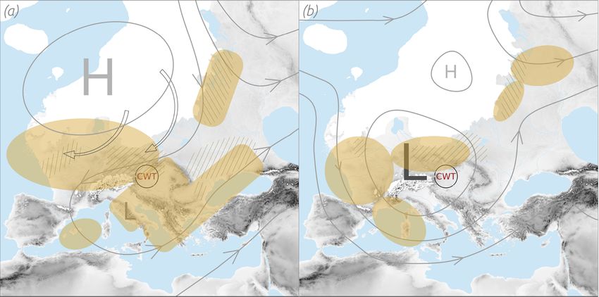
4970 E. J. Schaffernicht et al.: Linkage between LGM dust cycle and loess in Europe
land surfaces and biome types favoured more dust storms and
transport over Europe (Újvári et al., 2012).
Loess as a palaeoclimate proxy provides one of the
most complete continental records for characterizing climate
change and evaluating palaeoclimate simulations (Singhvi
et al., 2001; Haase et al., 2007; Fitzsimmons et al., 2012;
Varga et al., 2012). In Europe, loess covers large areas
with major deposits centred around 50◦ N (Antoine et al.,
2009b; Sima et al., 2013). However, although numerous Eu-
ropean loess sequences date to the LGM, it is not well un-
derstood where the dust that contributed to the loess for-
mation originated (Fitzsimmons et al., 2012; Újvári et al.,
2017). There are various hypotheses for the potential dust
sources, yet they are not fully tested because the dust cycle
of the LGM is neither well understood nor quantified. The
use of loess as a proxy for palaeoclimate reconstruction is
considerably compromised because the linkage between the
loess deposits and the responsible physical processes is un-
clear (Újvári et al., 2017). Reliable palaeodust modelling is
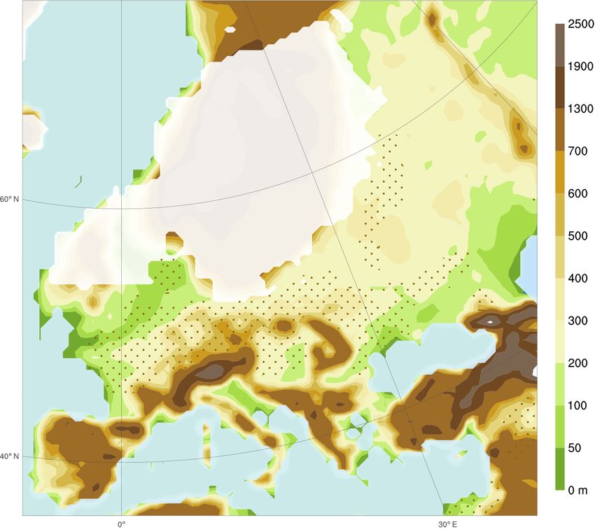
Figure 1. Simulation domain showing the applied topography
a promising way to establish this linkage and strengthen the (shaded), the potential dust source areas (dots), and the Eurasian
physical basis for palaeoclimate reconstructions using loess ice sheet extent (white overlay, adapted from Cline et al., 1984) of
records. Such attempts have been made for example by An- the Last Glacial Maximum.
toine et al. (2009b), who analysed the Nussloch record. They
suggested that rapid and cyclic aeolian deposition due to cy-
clones played a major role in the European loess formation Jungclaus et al., 2012, 2013; Giorgetta et al., 2013; Stevens
during the LGM. et al., 2013). This model was chosen since its 1850–2005
However, significant discrepancies exist between the mass experiment reproduces the recent observed wind distribution
accumulation rates (MARs) of aeolian deposits that are esti- over Europe best compared to the other climate models (Lud-
mated from fieldwork samples and the dust deposition rates wig et al., 2016). In addition, the MPI-LGM provides three-
calculated by climate model simulations (Újvári et al., 2010). dimensional boundary conditions updated frequently enough
For Europe, the global LGM simulations result in dust depo- to carry out the intended WRF-Chem-LGM experiments.
sition rates (based on different particle size ranges) of less The WRF-Chem was chosen since it has already been eval-
than 100 g m−2 yr−1 (Werner, 2002; Mahowald et al., 2006; uated successfully in many recent studies comparing its dust
Hopcroft et al., 2015; Sudarchikova et al., 2015; Albani et al., simulations with observations (Bian et al., 2011; Kang et al.,
2016). These are substantially smaller than the MARs (on 2011; Zhao et al., 2011, 2012; Rizza et al., 2016; Baumann-
average: 800 g m−2 yr−1 ) that have been reconstructed from Stanzer et al., 2019). Therefore, it is likely that the newly
more than 70 different loess sites across Europe (Supplement created WRF-Chem-LGM will simulate the LGM dust emis-
Table S1). This underestimation is probably due to the coarse sion, transport, and deposition processes similarly well. This
resolution of the global models which ignores dust sources, capacity of the WRF-Chem-LGM allows the reduction of the
emission, transport, and deposition processes at the small discrepancies between the MARs and the simulation-based
scale (Werner, 2002). Other causes can be missing glacio- dust deposition rates. It enables the establishment of a link-
genic dust sources, a low dust model sensitivity, an underes- age between the glacial dust cycle and the on-site loess de-
timated source material availability (Mahowald et al., 2006; posits.
Hopcroft et al., 2015), a biased atmospheric circulation, and
a lack of dust storms and interannual variability (Hopcroft
et al., 2015; Ludwig et al., 2016). 2 Data and methods
For this study, we simulated the aeolian dust cycle in
Europe using a LGM-adapted version of the Weather Re- The WRF-Chem-LGM consists of fully coupled modules for
search and Forecasting Model coupled with Chemistry (Mar- the atmosphere, land surface, and air chemistry. The simu-
tina Klose, personal communication, 2014; Grell et al., 2005; lation domain encompasses the European continent includ-
Fast et al., 2006; Kang et al., 2011; Kumar et al., 2014; ing western Russia and most of the Mediterranean (Fig. 1)
Su and Fung, 2015) referred to as the WRF-Chem-LGM. discretized by a grid spacing of 50 km and 35 atmospheric
The boundary conditions for the WRF-Chem-LGM simula- layers. The domain boundary conditions were updated ev-
tions are provided by the LGM simulation (MPI-LGM) of ery 6 h by using the MPI-LGM. The sea surface temperature
the Max Planck Institute Earth System Model (MPI-ESM; and sea ice cover are updated daily based on the correspond-
Atmos. Chem. Phys., 20, 4969–4986, 2020 www.atmos-chem-phys.net/20/4969/2020/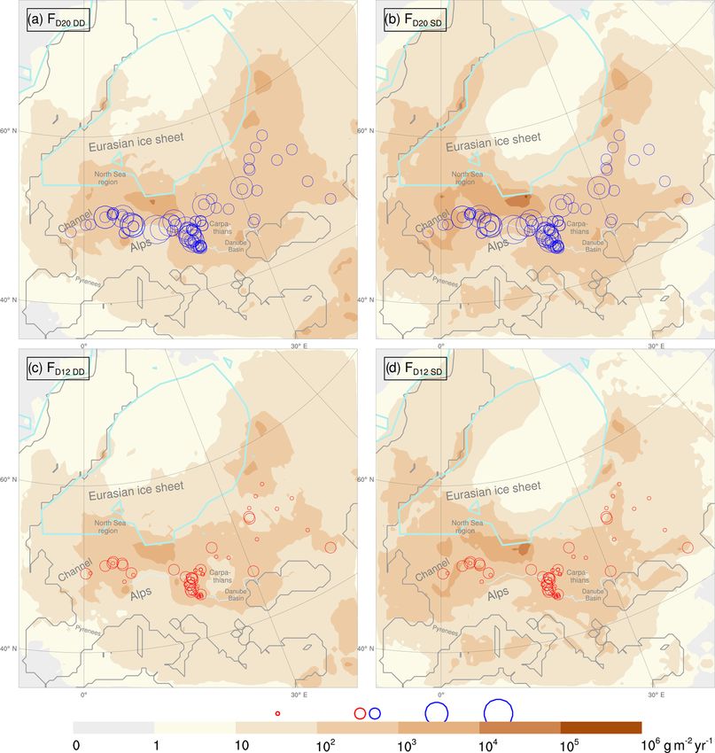
E. J. Schaffernicht et al.: Linkage between LGM dust cycle and loess in Europe                                                         4971

Table 1. Temporal concept for the episodic 8 d WRF-Chem-LGM simulations performed to reconstruct the LGM dust cycle based on
statistic dynamic downscaling. As the MPI-LGM contains fewer than 13 separate 8 d record sequences for a few CWTs, some of the episodes
were driven by a heterogeneous sequence of records. That is, one (or more) of the records in these sequences differs in its CWT from the
CWT of the records for the main days. For selecting heterogeneous sequences, the CWT correspondence between the main and tracking
records is considered higher priority (= ++ ) than between the main and spin-up records (= + ).

                          Days     Preferences for selecting record series from the MPI-LGM
              Spin-up         2    Prefer+ sequences whose spin-up records have the same CWT as the main records
              ↓
              Main            3    All records that drive the main part (central 3 d) of each episode must be of the same CWT
              ↓
              Tracking        3    Prefer++ sequences whose tracking records have the same CWT as the main records

Figure 2. Conceptual model explaining the linkage between the European dust cycle during the Last Glacial Maximum and the loess deposits.
The main dust deposition areas (filled), emission areas (hatched), and wind (grey lines) and pressure patterns (H or L: high or low pressure)
are highlighted; all of them result from the WRF-Chem-LGM experiments. The centre of the region for the circulation weather type analysis
is denoted by CWT. (a) Northeasters, easterlies, and southeasters (the east sector winds; transparent arrows with black perimeter) caused
by the semi-permanent high pressure over the Eurasian ice sheet (white) prevailed 36 % of the time over central Europe (Table 2). (b) The
cyclonic weather type regimes which prevailed 22 % of the time over central Europe (Table 2).

ing MPI-LGM variables. To simulate the dust cycle including              to the 50 km grid and converted (Ludwig et al., 2017) to
dust emission, transport, and deposition, the dust-only mode             the WRF-compatible United States Geological Survey cat-
of the WRF-Chem-LGM was selected. This mode implies                      egories (USGS-24) to replace their present-day analogues.
the application of the size-resolved (dust size bins: 0–2, 2–            The relative vegetation seasonality during the LGM is as-
3.6, 3.6–6, 6–12, and 12–20 µm) University of Cologne dust               sumed to resemble that of the present. Based on this unifor-
emission scheme (Shao, 2004), the Global Ozone Chemistry                 mitarianism approach, the CLIMAP maximum LGM vege-
Aerosol Radiation Transport (GOCART; Chin et al., 2000,                  tation cover reconstruction (Cline et al., 1984) was weighted
2002; Ginoux et al., 2001, 2004), and the dry and the wet                using the corresponding monthly fractions of the present-
deposition modules (Wesely, 1989; Chin et al., 2002; Grell               day WRF maximum vegetation cover and prescribed in the
et al., 2005; Jung et al., 2005).                                        model.
   To replace the present-day WRF surface boundary con-                     The erodibility at point p during the LGM is approximated
ditions with the LGM conditions, the data sets for the                   by
global 1◦ resolved land–sea mask and the topography off-
                                                                                  zmax − z 5

set provided by PMIP3 (Paleoclimate Model Intercompari-                  S=                     ,                                  (1)
son Project Phase 3; Braconnot et al., 2012) were interpo-                      zmax − zmin
lated to the 50 km grid (Fig. 1, Tables S2 and S3). To rep-              with z being the LGM terrain height at p and zmin (zmax )
resent the LGM glaciers and land use, the 2◦ CLIMAP re-                  representing the minimal (maximal) height in the 10◦ × 10◦
constructions (Climate: Long range Investigation, Mapping,               area centred around p (Ginoux et al., 2001). Setting S to zero
and Prediction; Cline et al., 1984) were also interpolated               where the CLIMAP bare soil fraction reconstruction is less

www.atmos-chem-phys.net/20/4969/2020/                                                      Atmos. Chem. Phys., 20, 4969–4986, 2020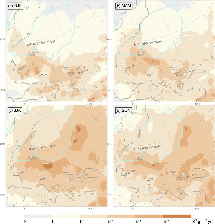
4972                                        E. J. Schaffernicht et al.: Linkage between LGM dust cycle and loess in Europe

than 0.5 refines this approximation. The adapted University        up days and excluded. The reconstruction of quantity Q us-
of Cologne dust emissions scheme takes into account that           ing statistic dynamic downscaling is then calculated from the
the erodibility exceeds a lower limit of 0.09 for emission to      weighted ensemble mean (Reyers et al., 2014):
occur. This suppresses dust sources in areas that had been                 X fi Z
attributed small physically meaningless interpolation-caused       hQi =            Q(t)dt,                                  (2)
erodibility artefacts. The vegetation and snow cover are                     i
                                                                                T
                                                                                   T
considered mutually independent and uniformly distributed
within a grid cell; i.e. the erodible area is multiplied by the    with i representing the ith CWT, fi its occurrence frequency,
fractional factor (1 − csnow ) to account for snow cover.          and T its duration. To evaluate the simulations, the obtained
   To simulate the LGM dust cycle with the WRF-Chem-               dust deposition rates are compared to more than 70 indepen-
LGM, two downscaling approaches of the MPI-LGM were                dent MARs reconstructed from loess sites located in the sim-
implemented: the dynamic downscaling approach and the              ulation domain (Table S1).
statistic dynamic downscaling approach. Both emerge from
simulations that are based on identically configured numer-
ical schemes representing the atmospheric chemistry and            3     Results
physics in the WRF-Chem-LGM. Using dynamic down-
                                                                   3.1    Dust cycle hypothesis
scaling, a consecutive 30-year simulation (corresponding to
more than 10 000 d) was performed. In contrast, the statis-        In line with previous modelling (COHMAP Members, 1988;
tic dynamic downscaling is based on 130 mutually inde-             Ludwig et al., 2016) and fieldwork studies (Dietrich and See-
pendent episodes each spanning 8 d, or a total of 1040 d.          los, 2010; Krauß et al., 2016; Römer et al., 2016), we hypoth-
The episode selection relies on the circulation weather type       esize that east sector winds (i.e. northeasters, easterlies, and
(CWT) classification (Jones et al., 1993, 2013; Reyers et al.,     southeasters) dominated the mineral dust cycle over central
2014; Ludwig et al., 2016) of the MPI-LGM records into 10          Europe during the LGM (Fig. 2). This hypothesis also im-
classes: cyclonic, anticyclonic, northeasterly, easterly, south-   plies a linkage of dust sources in central and eastern Europe
easterly, southerly, southwesterly, westerly, northwesterly,       during the LGM and the loess deposits in Europe. It is sug-
and northerly. The CWT classification approach is chosen           gested here that a greater proportion of all LGM dust deposits
since the atmospheric circulation patterns are the dominant        in central and eastern Europe comes more from sources in
factor for controlling dust emission from and deposition on        central and eastern Europe than from sources in the English
dry, low, and sparsely vegetated soil surfaces (Ginoux et al.,     Channel. The east sector winds likely contributed substan-
2001; Darmenova et al., 2009; Shao et al., 2011a, b). Such         tially to the formation of the European loess belt in central
surfaces characterized the unglaciated regions in central and      Europe. Among them, the northeasters and easterlies origi-
eastern Europe during the LGM (Ugan and Byers, 2007). To           nated most likely from dry winds that flowed down the slopes
compare the prevailing wind directions over Europe during          of the southern and eastern EIS margins, where they picked
the pre-industrial (PI) period and the LGM, the daily mean         up and turned gradually into northeasters and easterlies. By
sea level pressure patterns (interpolated to 2.5◦ horizontal       blowing over the bare proglacial EIS areas, they generated
grid spacing) of the MPI-LGM and the MPI-ESM simula-               dust emissions and carried the dust westwards, implying dust
tion for the PI period (MPI-PI) were classified for the region     depositions in areas west of the respective dust sources.
centring around (47.5◦ N, 17.5◦ E). For records showing ro-
tational and directional CWT patterns, only the directional        3.2    East sector winds and cyclones over central Europe
pattern is counted. By counting and statistically evaluating
the CWTs of all records, a LGM and a PI CWT occurrence             In agreement with this hypothesis, glacial simulations for
frequency distribution are established. The LGM distribution       90 kyr ago evidenced katabatic winds over the EIS (Krin-
served to reconstruct the LGM dust cycle using statistic dy-       ner et al., 2004), and global climate model (GCM) simu-
namic downscaling. It also enabled the analysis of the con-        lations for the LGM indicate prevailing east sector winds
tributions of each wind regime to the dust cycle.                  over central and eastern Europe (COHMAP Members, 1988;
   For the statistic dynamic downscaling, we performed             Ludwig et al., 2016). In Germany, several aeolian sediment
130 WRF-Chem-LGM simulations in total, i.e. 13 simula-             records that are dated to the LGM originated from more east-
tions for each of the 10 CWT classes. For each of these 8 d        ern sources (Dietrich and Seelos, 2010; Krauß et al., 2016;
simulations, independent consecutive sequences of boundary         Römer et al., 2016). The CWT frequencies for the present
conditions were chosen out of all MPI-LGM records of the           (not shown) and the PI era are very similar; therefore it is pos-
same CWT class. For CWTs with too few sets of distinct             sible to use the term present day to refer to both the PI and the
consecutive MPI-LGM records of the required CWT, the re-           actual present-day frequencies. In contrast to the dominant
maining sets were chosen applying less strict selection cri-       present-day anticyclones and west sector winds (southwest-
teria (Table 1). For the analysis of all performed episodic        ers, westerlies, and northwesters), east sector winds (36 %)
simulations, the first 2 d of each episode are considered spin-    and cyclones (22 %) prevailed over central Europe during

Atmos. Chem. Phys., 20, 4969–4986, 2020                                                www.atmos-chem-phys.net/20/4969/2020/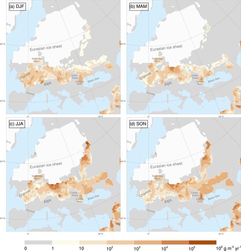
E. J. Schaffernicht et al.: Linkage between LGM dust cycle and loess in Europe                                               4973

Figure 3. Dust emission rates for the Last Glacial Maximum. These reconstructions are based on (a) dynamic downscaling (DD) and
(b) statistic dynamic downscaling (SD). Ice sheet extents (white overlay) and Danube (light-blue line).

the LGM (Table 2). The east sector winds are associated            dant in the Dehner Maar sediments (Eifel, Germany, 50.3◦ N,
with a strong EIS high (Fig. 2a and COHMAP Members,                6.5◦ E; Dietrich and Seelos, 2010). Their provenance showed
1988). The increased frequency of cyclones over central Eu-        that up to every fifth dust storm over the Eifel came from the
rope is consistent with the analysis of the LGM storm tracks,      east (Dietrich and Seelos, 2010).
which deviated from their present-day course (Hofer et al.,           Our findings are in agreement with fieldwork-based re-
2012), running either along central Europe, the Mediter-           sults of Römer et al. (2016), who found evidence for strong
ranean, or the Nordic Seas (Florineth and Schlüchter, 2000;        east sector winds over northern, central, and western Ger-
Luetscher et al., 2015; Ludwig et al., 2016). Their Mediter-       many for 23 to 20 kyr ago. Also, loess in the Harz Fore-
ranean course is consistent with the Alpine, western, and          land indicates a shift to prevailing east sector winds for the
southern European climate proxies (Luetscher et al., 2015).        LGM (Krauß et al., 2016). The location of aeolian ridges
In addition, the proxies indicate a storm track branch split-off   along rivers in northeastern Belgium and a core transect
over the Adriatic that ran past the Eastern Alps to central Eu-    near Leuven also support our finding by evidencing north-
rope (Florineth and Schlüchter, 2000; Luetscher et al., 2015;      easters for the Late Pleniglacial (Renssen et al., 2007). In
Újvári et al., 2017). These proxy-based findings are in line       addition, northerlies, northeasters, and easterlies were in-
with the more frequent cyclones in central Europe during the       ferred from loess deposits west of the Maas (Renssen et al.,
LGM (Table 2). This, in turn, can be related to the stronger       2007). Also, for Denmark, wind-polished boulders evidence
and southward-shifted jet stream (Luetscher et al., 2015;          dominant easterlies and southeasters in the period of 22
Ludwig et al., 2016) and the missing Scandinavian cyclone          to 17 kyr ago (Renssen et al., 2007). The CWT frequency
tracks, which were deflected southwards by the blocking EIS        distribution for the LGM (Table 2) contradicts the find-
high. As a result, their frequency increased over central Eu-      ing (Renssen et al., 2007) of prevailing west sector winds
rope (Table 2), consistent with susceptibility- and grain-size-    during the LGM in central Europe (40–55◦ N, 0–30◦ E). The
based results that suggest more frequent storms over western       distribution also contrasts with the finding (Sima et al., 2013)
Europe. The east sector winds, which more than doubled in          of prevailing winds from the west-northwest in eastern cen-
frequency in comparison to today (36 % compared to 17 %,           tral Europe, in particular for the area around Stayky (50◦ N,
Table 2), need to be incorporated to establish a more com-         31◦ E). More precisely, the CWT-W and CWT-NW regimes
plete understanding of the main drivers of the dust cycle in       occurred in eastern central Europe in total less than 10 % of
Europe during the LGM (Fig. 9a). These winds are also ev-          the times during the LGM (Table 2), which is even less than
idenced by northern-central European grain size records for        the expectation value for a single weather type in the case of a
the Late Pleniglacial (Bokhorst et al., 2011). Sediment lay-       uniform CWT frequency distribution. Conversely, the signif-
ers attributed to east wind dated to 36–18 kyr BP are abun-        icant role of the east sector winds (Table 2) is consistent with

www.atmos-chem-phys.net/20/4969/2020/                                               Atmos. Chem. Phys., 20, 4969–4986, 2020
4974                                               E. J. Schaffernicht et al.: Linkage between LGM dust cycle and loess in Europe

Table 2. Circulation weather type occurrence frequencies (%) for central Europe (centred at 17.5◦ E and 47.5◦ N) during the LGM and the
pre-industrial period (PI). The frequencies are based on the LGM and the PI simulation of the Max Planck Institute Earth System Model. The
circulation weather type classes are cyclonic (C), anticyclonic (A), northeasterly (NE), and easterly (E) followed by the remaining standard
wind directions.

                                          C          A       NE           E      SE         S     SW       W     NW           N
                              LGM       22.2        8.9     12.4     13.4       10.2       9.7     6.8    4.3     5.0    7.0
                              PI        10.6       24.1      7.3      5.2        4.9       7.6    11.6   11.1     9.4    8.3

Table 3. Seasonal CWT occurrence frequencies (%) for central Europe (centred at 17.5◦ E and 47.5◦ N) during the LGM. The frequencies
are based on MPI-LGM simulation. The CWT classes are cyclonic (C), anticyclonic (A), northeasterly (NE), and easterly (E) followed by
the remaining standard wind directions. Sum E is the sum of the east sector winds (NE, E, SE). The seasons are labelled DJF (winter), MAM
(spring), JJA (summer), and SON (autumn).

                                    C          A     Sum E         NE           E          SE      S     SW     W       NW          N
                        DJF      12.6     13.9            37.4     11.8       14.4     11.2      12.9    8.5    5.1     4.1        5.6
                        MAM      27.1      6.1            41.9     12.9       16.4     12.6       9.7    4.8    2.8     3.6        4.2
                        JJA      26.8      7.5            24.4     12.8        6.3      5.3       9.3    7.3    6.1     7.9       10.7
                        SON      18.6     10.0            37.8     12.8       13.6     11.4      10.8    6.8    3.8     5.1        7.0

the deposits on the west bank of the Dnieper (Sima et al.,                           a dust source and a dust sink (Figs. 3 and 4). Major dust
2013), which are also the loess deposits closest to Stayky.                          sources surrounding the Carpathians and the Eastern Alps
In addition, sandy soil texture and sand dunes indicate pre-                         (Fig. 3) are in line with deposits in Serbia and the Carpathian
vailing northerlies and northeasters over Dobrudja (44.32◦ N,                        Basin (Újvári et al., 2010; Bokhorst et al., 2011). The dust
28.18◦ E), the eastern Wallachian Plain (both located in Ro-                         emissions from the Lower Danube Basin (Fig. 3) are in
mania), and Stary Kaydaky (Ukraine, 48.37◦ N, 35.12◦ E;                              agreement with plentiful sediment supply, strong winds, and
Buggle et al., 2008). The northerlies over Ukraine origi-                            dry conditions inferred from the plateau loess in Urluia, lo-
nated from katabatic winds descending from the EIS (Buggle                           cated near the Black Sea in southeastern Romania (Fitzsim-
et al., 2008). The high aridity and grain size variations in the                     mons and Hambach, 2014). Also, the emissions from the
Surduk (Serbia, Table S1) and Stari Bezradychy (Ukraine,                             western Black Sea littoral (Fig. 3) are consistent with prove-
Table S1) records evidence prevailing dry and periodically                           nance analyses of eastern Dobrogea loess in the Lower
strong east sector winds (Antoine et al., 2009a; Bokhorst                            Danube Basin (Jipa, 2014). Our results indicate a close rela-
et al., 2011).                                                                       tionship between strong dust emissions and low terrains (or
                                                                                     basins). This relationship is found for the North Sea Basin
3.3    Dust emissions from the Eurasian ice sheet margin                             and the European plains bordering the EIS, the Caucasus, the
                                                                                     Carpathians, or the Massif Central (Figs. 1 and 3). The dust
The model-simulated dust emission (Fig. 3) indicates that                            emissions from the EIS margin and from the foothills of the
most dust in Europe was emitted from the less elevated cor-                          European mountains (Fig. 3) are consistent with the loess-
ridor between the Alps, the Black Sea, and the EIS (45–                              based finding of significant aeolian dust contributions from
55◦ N). This finding is consistent with loess-based dust flux                        glaciogenic and orogenic dust sources (Újvári et al., 2010).
estimates (Újvári et al., 2010). The highest emission rates
(> 105 g m−2 yr−1 ) occurred along the southern EIS margin                           3.4    Conforming dust deposition and loess
(51–53◦ N, 15–18◦ E, Fig. 3). This location is in line with                                 accumulation rates
the location of the highest emissions found in the Greenland
stadial GCM simulation of Sima et al. (2013); yet our sim-                           Compared with the GCMs (Werner, 2002; Mahowald et al.,
ulation indicates a larger upper limit for the emission rates                        2006; Hopcroft et al., 2015; Sudarchikova et al., 2015; Al-
(1000 g m−2 yr−1 ). Our results also show high emissions in                          bani et al., 2016), the WRF-Chem-LGM dust deposition rates
the dried-up English Channel and the German Bight (Fig. 3).                          (FD , Fig. 4) reproduce the MARs (Table S1, Fig. 4a and b)
For the latter, they compare well with the average emission of                       and MAR10 (Table S1, Fig. 4c and d) better, at least by
140 and the maximum emission greater than 200 g m−2 yr−1                             1 order of magnitude. One factor for this improvement is
based on a glacial climate simulation (Sima et al., 2009).                           most likely the higher spatio-temporal resolution (Ludwig
   The loess deposits (Újvári et al., 2010) and the model re-                        et al., 2019) of the WRF-Chem-LGM experiments combined
sults are consistent in that the Carpathian Basin was both                           with the provided more highly resolved geographical input

Atmos. Chem. Phys., 20, 4969–4986, 2020                                                                  www.atmos-chem-phys.net/20/4969/2020/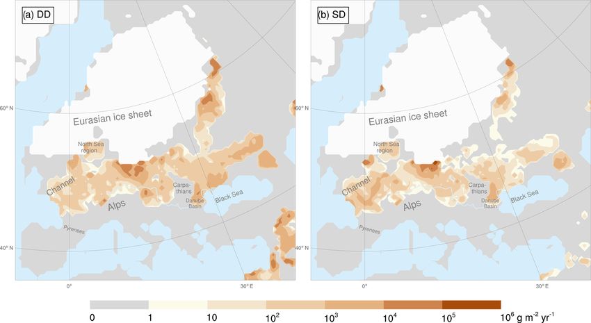
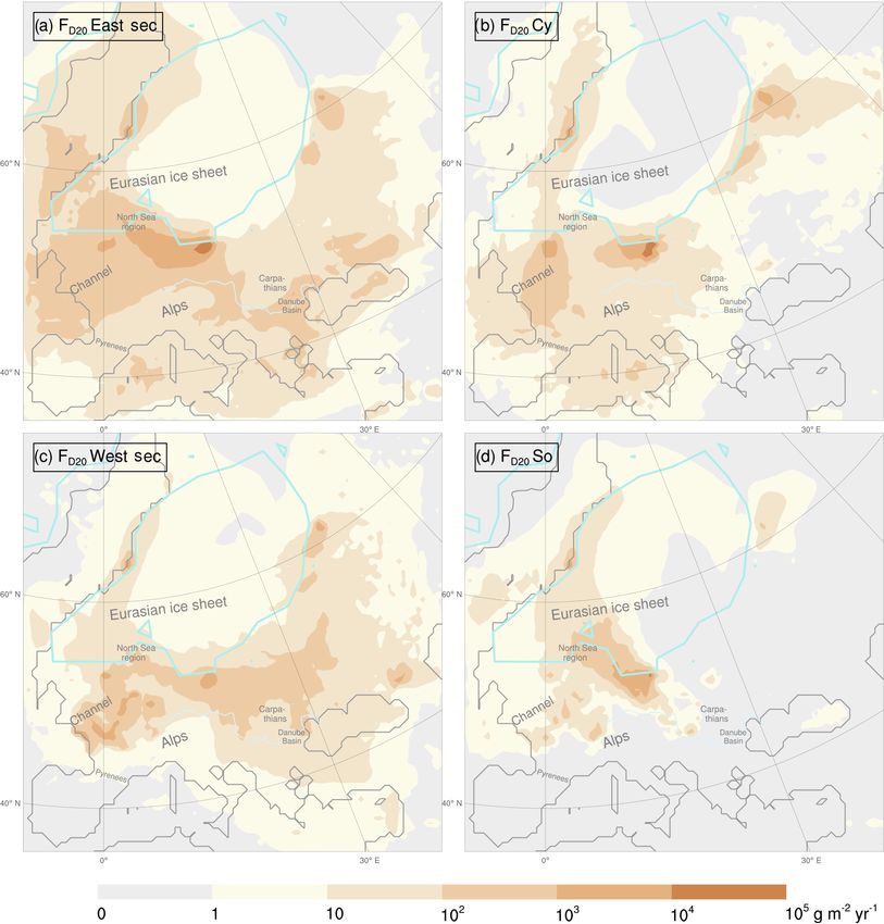
E. J. Schaffernicht et al.: Linkage between LGM dust cycle and loess in Europe                                                 4975

data, for example the regional LGM topography, land use,             French LGM coastline (46–48◦ N), on the eastern side of
and dynamic (yet monthly prescribed) vegetation cover. The           the Carpathians (44–47◦ N, including the eastern Romanian
boundary conditions provided by the MPI-LGM could also               Danube Plain), and near the Caucasus (44–45◦ N, Fig. 4a).
be a factor for this improvement. Taking into account that           They coincide with today’s extensive loess derivates along
the MPI-ESM experiment for the present reproduces the ob-            the Atlantic coastline of France and at the European foothills
served atmospheric circulation over Europe better than other         north of 42◦ N, with the loess thickness maximum in the
GCMs (Ludwig et al., 2016), it is likely that MPI-LGM also           Romanian Danube Plain (Haase et al., 2007; Jipa, 2014).
reproduces the LGM conditions more realistically. Another            The quality of the simulations is also recognizable in the
factor could be the orography-based estimated fraction of al-        Carpathian Basin, which is now half covered with loess and
luvium (Ginoux et al., 2001) combined with the proxy-based           clay of aeolian origin (Varga et al., 2012). There, the sim-
reconstructed bare soil fraction (Cline et al., 1984) to calcu-      ulated FD20 values of 100–1000 g m−2 yr−1 (Fig. 4a) are in
late the spatial erodibility distribution. Based on this distribu-   good agreement with the MARs (200–500 g m−2 yr−1 ). In
tion, the WRF-Chem-LGM was able to suppress unrealistic              Ukraine and at the eastern margins of the EIS, FD20 values
numerical dust emission from areas with low or zero erodibil-        of 100–1000 g m−2 yr−1 are in line with the MARs (Fig. 4a).
ity. Most likely, the improvement also results from selecting        Over Ukraine and consistent with our results, dust transport
the well-tested and observation-confirmed Shao dust emis-            and deposition by east sector winds are evidenced by loess
sion scheme (Shao, 2004; Kang et al., 2011). For example,            deposits on the west bank of the Dnieper (Sima et al., 2013).
this scheme takes into account the dynamic moisture changes             The MARs of a few loess sites are higher than the FD20
at the soil surface. Due to our recent improvement of the            in their surroundings. Such an underestimation could be ex-
Shao dust emission scheme, the effect of snow cover on dust          plained by particles larger than 20 µm, which are not taken
emission has also been taken into account in the WRF-Chem-           into account by the FD20 . For some regions, the MARs of
LGM experiments.                                                     closely related sites vary over orders of magnitude, e.g. be-
   The MARs and MAR10 (Table S1 and Fig. 4) were re-                 tween 102 and 104 g m−2 yr−1 near the Rhine and in Bel-
constructed from samples that were extracted during field-           gium (Fig. 4a). This may be due to strong small-scale
work campaigns from loess paleosol sites. The MAR for a              variability, loess dating uncertainties (Singhvi et al., 2001;
specific site was inferred by taking into account all particles      Renssen et al., 2007), or age model inaccuracies (Bettis et al.,
found in the respective sample, independent of their diame-          2003). For western Germany, a transition from higher FD20
ter. In contrast, the MAR10 for the same site was inferred by        (103 –104 g m−2 yr−1 ) in the northeast to lower FD20 (102 –
taking into account only particles up to 10 µm in diameter.          103 g m−2 yr−1 ) in the southwest was found (Fig. 4a). For
Most of the MARs and MAR10 (Table S1 and Fig. 4) result              a few sites in southwestern Germany, Austria, Ukraine, and
from sites of the European loess belt. This belt plays a key         along the Danube, FD20 is an order of magnitude lower than
role in assessing palaeoclimatic dust cycle simulations for          the respective MARs (Fig. 4a). Given the 50 km grid spacing
Europe (Kukla, 1977; Little et al., 2002; Haase et al., 2007;        of the WRF-Chem-LGM simulation, this may be attributed
Sima et al., 2009). During the LGM, it corresponded approx-          to missing local dust sources, such as dried-up riverbeds and
imately to the fraction of the European land area that was           floodplains. Possibly, the MARs of these sites are also in-
bounded northwards by the EIS and southwards by the Alps,            ferred from particles that were predominantly larger than
Dinaric Alps, and Black Sea. The FD20 in Fig. 4a and b (FD12         20 µm, yet data on particle sizes are not available. The peak
in Fig. 4c and d) denotes the WRF-Chem-LGM deposition                deposition locations and the overall shape of the FD20 and
rates caused only by particles smaller than 20 µm (12 µm) in         FD12 patterns are very similar (Fig. 4). The FD12 values are
diameter. To distinguish the deposition rates obtained from          also consistent with the MAR10 almost everywhere (Fig. 4c
the two downscaling methods, the FD20DD and FD12DD re-               and d). Those FD12 values that overestimate the MAR10
late to the dynamic, while the FD20SD and FD12SD relate to           do not contradict the consistency since the FD12 also takes
the statistic dynamic downscaling simulations.                       into account particles that are (by definition) excluded by
   For central Europe, the dynamic (Fig. 4a and c) and statis-       the MAR10. In summary, high consistency was found be-
tic dynamic downscaling (Fig. 4b and d) resulted in similar          tween the simulated dust deposition rates and the MARs and
FD values, confirming the suitability of the statistic dynamic       MAR10 that were reconstructed from on-site samples.
downscaling.
   During the LGM, the largest FD20 (> 105 g m−2 yr−1 ) oc-          3.5   Seasonal dust cycle patterns
curred in western Poland (Fig. 4a). Slightly lower FD20 val-
ues (104 –105 g m−2 yr−1 ) were found in adjacent areas, in          During the LGM, the strongest emission and deposition in
eastern Germany, for example. FD20 was 103 –104 g m−2 yr−1           Europe occurred in summer, followed by autumn and spring
on the North German Plain, in the dried-up German Bight,             (Figs. 5 and 6). The areas with the overall highest emis-
eastern England, northern and western France, the Benelux            sion were also those with the highest seasonal emission
region, and southeast of the Carpathians. Regional depo-             (Figs. 3 and 5). The spring and winter emissions have the
sition maxima of 103 –104 g m−2 yr−1 occurred along the              same order of magnitude. The low winter and spring emis-

www.atmos-chem-phys.net/20/4969/2020/                                                 Atmos. Chem. Phys., 20, 4969–4986, 2020
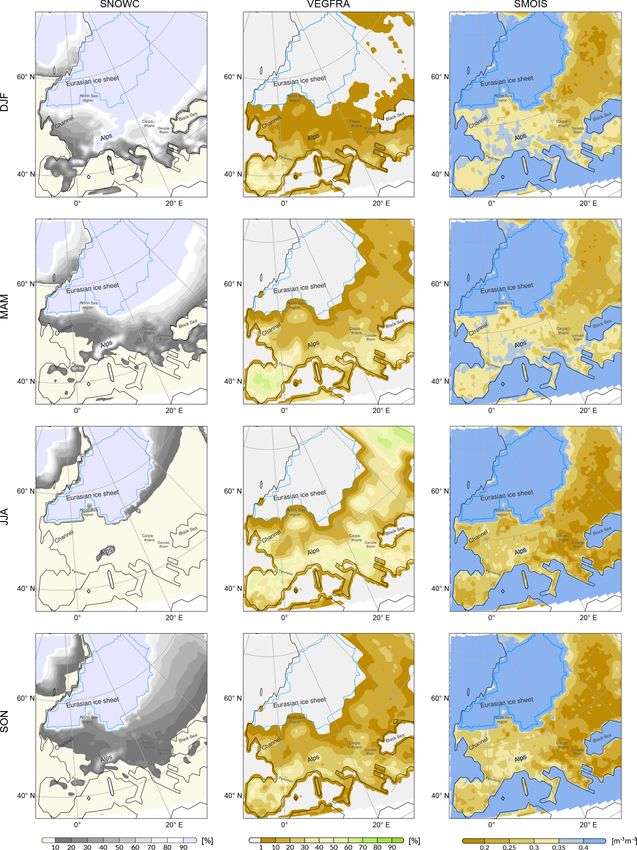
4976                                         E. J. Schaffernicht et al.: Linkage between LGM dust cycle and loess in Europe

Figure 4. Dust deposition rates for the Last Glacial Maximum, comprising particles of up to 20 µm in diameter (FD20 ) using (a) dy-
namic downscaling (FD20DD ) and (b) statistic dynamic downscaling (FD20SD ). Panels (c) and (d) are as (a) and (b), but for particles up to
12 µm (FD12 ). Each blue circle size represents one mass accumulation rate (MAR, Table S1 column 5) magnitude. Each red circle size
represents one reduced mass accumulation rate (MAR10, Table S1 column 6) magnitude. MAR and MAR10 values compiled in Table S1.
The simulation-based (FD20 , FD12 ) and the fieldwork-based (MAR, MAR10) rates result from independent data. Delineated are the Danube
(light blue), the coastlines (grey; Braconnot et al., 2012), and the ice sheet extents (turquoise; Cline et al., 1984).

sion rates along the EIS margin were caused by the then ex-             For eastern Europe, the growing vegetation cover and the
tensive snow cover there. During winter, emissions peaked               slight soil moisture increase account for partly lower spring
only in northern France, consistent with its little snow cover          than winter emission rates. The soil moisture increase pos-
and the vegetation cover (Fig. 7) that was prescribed to the            sibly resulted from meltwater of the retreating snow cover.
WRF-Chem-LGM. Major dust emissions occurred from the                    The highest emission rates occurred during summer and were
Carpathian Basin and along the northwest coast of the Black             located along the German and Polish EIS margin. Slightly
Sea. During spring, slightly attenuated emissions are simu-             lower emissions are found to the east of the EIS. These find-
lated for France, despite the decreasing snow cover but in ac-          ings are in coherence with the surface properties of these ar-
cordance with its increasing vegetation cover. Considerably             eas during summer, i.e. they were mostly snow free and the
higher emission rates are simulated from along the German               least moist. During autumn, the snow cover increased, caus-
and Polish EIS margin where the snow cover had retreated.               ing a decrease in dust emissions, except for the area north of

Atmos. Chem. Phys., 20, 4969–4986, 2020                                                   www.atmos-chem-phys.net/20/4969/2020/
E. J. Schaffernicht et al.: Linkage between LGM dust cycle and loess in Europe                                                   4977

Figure 5. Dust emission rates for (a) winter (DJF), (b) spring (MAM), (c) summer (JJA), and (d) autumn (SON) during the Last Glacial
Maximum. This reconstruction is based on dynamic downscaling. The Danube (light-blue line) and the extent of the continental ice sheets
(white) are shown.

the Black Sea which encountered its annual maximum. This              for southern France; however marked depositions occurred
maximum can be attributed to the retreat of the vegetation            when subjected to cyclonic regimes (Fig. 9b). The deposition
cover and the dry soil conditions there.                              pattern for the central Mediterranean area (Italy, the Adri-
   The winter CWT distribution indicates prevailing east sec-         atic) suggests significant dust transport by east sector winds
tor winds (37 %) in contrast to cyclonic regimes, which oc-           and anticyclonic winds, in sum prevailing 51 % of the time.
curred much less frequently than on an annual average (13 %;          In eastern Europe, considerable winter deposition rates cov-
Tables 2 and 3). The winter deposition rates northwest of the         ered areas south of the dust sources, in particular the western
Alps were considerably above the annual average, while the            Black Sea and regions south of the Danube. This indicates
rates at the central and eastern European EIS margin were             a significant contribution to the dust transport by norther-
below the annual average (Figs. 4 and 6a). In western Eu-             lies (6 %), northeasters (12 %), and the anticyclonic regimes
rope, the highest deposition rates occurred near the sources,         (14 %).
yet a considerable dust fraction was also transported and de-            Also, the spring deposition rates evidence the importance
posited to the west and northwest of the sources, which re-           of the east sector winds (42 %, Table 2) for the dust cycle.
quires east sector winds. Low deposition rates were found             In western Europe, major deposition areas are to the west

www.atmos-chem-phys.net/20/4969/2020/                                                  Atmos. Chem. Phys., 20, 4969–4986, 2020
4978                                         E. J. Schaffernicht et al.: Linkage between LGM dust cycle and loess in Europe

Figure 6. Dust deposition rates for (a) winter (DJF), (b) spring (MAM), (c) summer (JJA), and (d) autumn (SON) during the Last Glacial
Maximum. This reconstruction is based on dynamic downscaling. Ice sheet extents (turquoise; Cline et al., 1984), Danube (light-blue line),
and coastlines (grey; Braconnot et al., 2012) are delineated.

and northwest of the sources, while they are to the west and           gin over Germany and Poland, corroborating the major role
southwest in eastern Europe (Fig. 6b). An increase in the dust         of the east sector winds (38 %) in the dust cycle. The high
transport towards the south in western Europe and towards              deposition rates in eastern Europe suggest that the cyclonic
the north in eastern Europe indicates an increasing role of            regimes (19 %) also contributed during autumn.
the cyclonic regimes (27 %) during the spring.
   The summer deposition rates are distributed zonally                 3.6   Wind-regime-based dust cycle decomposition
along the EIS margin, suggesting an approximately latitude-
parallel dust transport by the west (21 %) and/or east sector          The wind regime occurrence frequency distribution (Ta-
(24 %) wind directions. In addition, the northern flanks of cy-        ble 2) demonstrates the temporal dominance of the east sec-
clonic regimes (24 %) likely contributed to a westward dust            tor winds during the LGM. This temporal dominance likely
transport. Over the northeasternmost part of Europe (62◦ N,            shaped the dust cycle but the contribution of each wind
40◦ E), the deposition rates suggest east sector winds. The            regime type has so far not been analysed. This analysis is
autumn deposition rates over western and central Europe                provided here by discussing the dust emission and deposi-
show a westward running plume from the southern EIS mar-               tion characteristics associated with different CWTs which
                                                                       reveal that the east sector winds caused by far the largest

Atmos. Chem. Phys., 20, 4969–4986, 2020                                                  www.atmos-chem-phys.net/20/4969/2020/
E. J. Schaffernicht et al.: Linkage between LGM dust cycle and loess in Europe 4979 Figure 7. Snow cover (%, left column), vegetation cover (%, centre), and soil moisture (m3 m−3 , right), resolved for winter (DJF), spring (MAM), summer (JJA), and autumn (SON) for the Last Glacial Maximum. These reconstructions are based on dynamic downscaling. www.atmos-chem-phys.net/20/4969/2020/ Atmos. Chem. Phys., 20, 4969–4986, 2020
4980                                          E. J. Schaffernicht et al.: Linkage between LGM dust cycle and loess in Europe

Figure 8. Dust emission rate fractions caused by the (a) northeasters, easterlies, and southeasters; (b) cyclonic regimes; (c) southwesters,
westerlies, and northwesters; and (d) southerlies during the Last Glacial Maximum. The simulated emission rates are weighted according to
the occurrence frequency of the associated wind regime(s) in the Max Planck Institute Earth System Model (Table 2). Dust particles up to
20 µm in diameter have been considered. The Danube (light-blue line) and the extent of the continental ice sheets (white) are shown.

dust emission and deposition during the LGM (Figs. 8a                   two near the EIS margin in western Russia. This distribu-
and 9a). In sum, they generated an average dust emission of             tion resembles a subset of the emission distribution of the
1111 g m−2 yr−1 (Fig. 8a), which is more than twice the rate            east sector winds (Fig. 8a). Together with the location of the
generated by cyclonic regimes (494 g m−2 yr−1 , Fig. 8b). The           CWT reference regions, this resemblance could be explained
west sector winds contributed on average even less to the dust          by the fact that all records classified as cyclonic must centre
cycle (375 g m−2 yr−1 , Fig. 8c). Compared to the southerlies           their cyclonic pressure distribution approximately around the
(232 g m−2 yr−1 , Fig. 8d), this rate is low for a wind sector          central point for the CWT classification (47.5◦ N, 17.5◦ E).
that sums the contribution of three wind directions (SW, W,             This implies that the corresponding emissions could have
NW).                                                                    been triggered by easterlies on the northern flanks of the cy-
   The cyclonic wind regimes caused the most heteroge-                  clones. Dust was hardly emitted from areas on the southern
neously distributed emissions (Fig. 8b) with four main cen-             flanks of the cyclones which are commonly affected by fronts
tres: the largest located in the German–Polish–Czech bor-               and precipitation (Booth et al., 2018). In addition to the dust
der region, another in eastern England, and the remaining               emission areas that occurred equally during both regimes

Atmos. Chem. Phys., 20, 4969–4986, 2020                                                    www.atmos-chem-phys.net/20/4969/2020/
E. J. Schaffernicht et al.: Linkage between LGM dust cycle and loess in Europe                                                           4981

Figure 9. Dust deposition rate fractions caused solely by the (a) northeasters, easterlies, and southeasters; (b) cyclonic regimes; (c) south-
westers, westerlies, and northwesters; and (d) the southerlies during the Last Glacial Maximum. The simulated deposition rates are weighted
according to the occurrence frequency of the associated wind regime(s) in the Max Planck Institute Earth System Model (Table 2). Dust
particles up to 20 µm in diameter have been considered. The ice sheet extents (turquoise; Cline et al., 1984), the Danube (light blue), and the
coastlines (grey; Braconnot et al., 2012) are delineated.

(cyclonic and east sector winds), the east sector winds also              sector winds (Figs. 8a and 9a) indicates major westward dust
generated emissions in Austria, Slovakia, Hungary, Ukraine,               transport along the southern and eastern EIS margin. The
central Germany, the Danube Basin, and the North Sea Basin.               conic shape of the deposition rate distribution in western and
In contrast, the west sector winds produced a more homo-                  central Europe (between 102 and 103 g m−2 yr−1 ) suggests
geneous distribution of markedly smaller emission rates ex-               that these depositions can be attributed to emissions from
tending from western Ukraine to the French Atlantic coast.                more eastern sources. The east sector winds also deposited
While northwesters with a strong northerly component most                 considerable amounts of dust in and south of the Danube
likely forced emissions from the German–Polish EIS mar-                   Basin as well as along the Danube.
gin, the west sector winds and the southerlies controlled the                The deposition rates of the cyclonic regimes (Fig. 9b) indi-
emissions from France, southwestern Germany, the English                  cate two main dust transport directions: westwards over cen-
Channel, and the Alps foreland (Fig. 8c and d). The combi-                tral and eastern Europe and southwards over western Europe.
nation of the emission and deposition rate patterns of the east           The shape and location of the emission and deposition ar-

www.atmos-chem-phys.net/20/4969/2020/                                                       Atmos. Chem. Phys., 20, 4969–4986, 2020
4982                                        E. J. Schaffernicht et al.: Linkage between LGM dust cycle and loess in Europe

eas caused by the west sector winds are almost congruent           due to the then-vanishing snow cover. The highest dust depo-
(Fig. 8c and 9c). This implies that a unique dust transport di-    sition rates during the LGM occurred near the southernmost
rection cannot be inferred for this wind regime. Instead, dust     margin of the EIS (12–19◦ E; 105 g m−2 yr−1 ), on the North
may have been transported in various directions. Dust depo-        German Plain including adjacent regions, and in the south-
sition in Ireland, western Great Britain, the Bay of Biscay,       ern North Sea region. The agreement between the performed
and near the eastern margin of the EIS even suggests a west-       climate–dust simulations for the LGM and the reconstructed
ward dust transport (Fig. 9c), implying that east sector winds     MARs from loess deposits corroborates the proposed LGM
may have occurred locally while possibly weak west sector          dust cycle hypothesis.
winds prevailed over central Europe. More precisely, dust
was transported westwards from Poland to eastern and cen-
tral Germany, while it was carried southwards from eastern         Data availability. Simulation results are available upon request
England to the English Channel and northwestern France up          from the authors.
to the Pyrenees foreland. The depositions caused by souther-
lies show a northwestward transport over central Europe
(Fig. 9d). Considerable amounts of dust (between 103 and           Supplement. The supplement related to this article is available on-
105 g m−2 yr−1 ) were transported from sources in western          line at: https://doi.org/10.5194/acp-20-4969-2020-supplement.
Poland, eastern Germany, and Czechia to northern Germany,
Denmark, southern Sweden, and the North Sea Basin. The
                                                                   Author contributions. EJS, PL, and YS designed the concept of the
deposition pattern also suggests a northwestward transport
                                                                   study. PL performed the dynamic downscaling simulation and cre-
in France.
                                                                   ated Fig. 7. EJS performed the statistic dynamic downscaling, com-
                                                                   pared the results with the proxy data including the reconstructed
                                                                   loess mass accumulation rates, and created the tables and the re-
4   Conclusions                                                    maining figures. EJS wrote the paper with contributions from PL
                                                                   and YS.
Compared to previous climate–dust model simulations for
the LGM, this study presents a dust cycle reconstruction with
dust deposition rates that are in much better agreement with       Competing interests. The authors declare that they have no conflict
the MARs reconstructed from more than 70 different loess           of interest.
deposits across Europe. By taking into account the effect of
different wind directions, a more complete understanding of
the dust cycle is established. The obtained results corrobo-       Acknowledgements. This research was funded by the Deutsche
rate the hypothesis on the linkage between the prevailing dry      Forschungsgemeinschaft (DFG) through the Collaborative Re-
east sector winds as a major driver of the LGM dust cycle in       search Center 806 “Our Way to Europe” (CRC806). Patrick Lud-
                                                                   wig thanks the Helmholtz initiative REKLIM for funding. We thank
central and eastern Europe and the loess deposits.
                                                                   the German Climate Computing Centre (DKRZ, Hamburg) for pro-
   The study demonstrates that the WRF-Chem-LGM model              viding the MPI-ESM data and computing resources (project 965).
is capable of simulating the glacial dust cycle including emis-    We thank the Regional Computing Center (University of Cologne)
sion, transport, and deposition. In addition, the suitability of   for providing support and computing time on the high-performance
the statistic dynamic approach for regional climate–dust sim-      computing system CHEOPS. We thank Qian Xia for preparing
ulations is proven by the similarity of the dynamic and statis-    model boundary condition data. We thank Frank Lehmkuhl, the
tic dynamic downscaling results. In contrast to the dominant       CRC806 (second phase) members of his group, and Joaquim Pinto
present-day westerlies over Europe, the CWT analysis re-           for helpful discussions and comments.
vealed dominant east sector (36 %) and cyclonic (22 %) wind
regimes during the LGM over central Europe. These east sec-
tor winds dominated the LGM dust cycle by far during all but       Financial support. This research has been supported by the
the summer season. In summer, they were about as frequent          Deutsche Forschungsgemeinschaft (DFG) (grant no. 57444011).
as the cyclonic regimes. The dominance of the east sector
winds during the LGM is corroborated by numerous local
proxies for the wind and dust transport directions in Europe.      Review statement. This paper was edited by Yves Balkanski and
                                                                   reviewed by two anonymous referees.
   The WRF-Chem-LGM simulations show that almost all
dust emission occurred in a corridor that was bounded to the
north by the EIS and to the south by the Alps and the Black
Sea. Within this corridor, the highest emissions were gener-       References
ated from the dried-up flats, the lowlands bordering mountain
slopes, and the proglacial areas of the EIS. Most dust was         Albani, S., Mahowald, N. M., Murphy, L. N., Raiswell, R., Moore,
emitted during summer and autumn in the LGM, probably                J. K., Anderson, R. F., McGee, D., Bradtmiller, L. I., Del-

Atmos. Chem. Phys., 20, 4969–4986, 2020                                              www.atmos-chem-phys.net/20/4969/2020/
E. J. Schaffernicht et al.: Linkage between LGM dust cycle and loess in Europe 4983 monte, B., Hesse, P. P., and Mayewski, P. A.: Paleodust vari- bia, Romania, Ukraine), Quaternary Sci. Rev., 27, 1058–1075, ability since the Last Glacial Maximum and implications for https://doi.org/10.1016/j.quascirev.2008.01.018, 2008. iron inputs to the ocean, Geophys. Res. Lett., 43, 3944–3954, Chin, M., Rood, R. B., Lin, S.-J., Müller, J.-F., and Thomp- https://doi.org/10.1002/2016GL067911, 2016. son, A. M.: Atmospheric sulfur cycle simulated in the Antoine, P., Rousseau, D.-D., Fuchs, M., Hatté, C., Gau- global model GOCART: Model description and global thier, C., Marković, S. B., Jovanović, M., Gaudenyi, T., properties, J. Geophys. Res.-Atmos., 105, 24671–24687, Moine, O., and Rossignol, J.: High-resolution record of https://doi.org/10.1029/2000JD900384, 2000. the last climatic cycle in the southern Carpathian Basin Chin, M., Ginoux, P., Kinne, S., Torres, O., Holben, B. N., (Surduk, Vojvodina, Serbia), Quatern. Int., 198, 19–36, Duncan, B. N., Martin, R. V., Logan, J. A., Higurashi, https://doi.org/10.1016/j.quaint.2008.12.008, 2009a. A., and Nakajima, T.: Tropospheric Aerosol Optical Antoine, P., Rousseau, D.-D., Moine, O., Kunesch, S., Hatté, C., Thickness from the GOCART Model and Comparisons Lang, A., Tissoux, H., and Zöller, L.: Rapid and cyclic aeolian with Satellite and Sun Photometer Measurements, J. deposition during the Last Glacial in European loess: a high- Atmos. Sci., 59, 461–483, https://doi.org/10.1175/1520- resolution record from Nussloch, Germany, Quaternary Sci. Rev., 0469(2002)0592.0.co;2, 2002. 28, 2955-2973, https://doi.org/10.1016/j.quascirev.2009.08.001, Clark, P. U. and Mix, A. C.: Ice sheets and sea level of 2009b. the Last Glacial Maximum, Quaternary Sci. Rev., 21, 1–7, Austermann, J., Mitrovica, J. X., Latychev, K., and Milne, G. A.: https://doi.org/10.1016/S0277-3791(01)00118-4, 2002. Barbados-based estimate of ice volume at Last Glacial Max- Clark, P. U., Dyke, A. S., Shakun, J. D., Carlson, A. E., Clark, imum affected by subducted plate, Nat. Geosci., 6, 553–557, J., Wohlfarth, B., Mitrovica, J. X., Hostetler, S. W., and Mc- https://doi.org/10.1038/ngeo1859, 2013. Cabe, A. M.: The Last Glacial Maximum, Science, 325, 710– Bartlein, P. J., Harrison, S. P., Brewer, S., Connor, S., Davis, B. 714, https://doi.org/10.1126/science.1172873, 2009. A. S., Gajewski, K., Guiot, J., Harrison-Prentice, T. I., Hender- Cline, R. M. L., Hays, J. D., Prell, W. L., Ruddiman, W. F., son, A., Peyron, O., Prentice, I. C., Scholze, M., Seppä, H., Shu- Moore, T. C., Kipp, N. G., Molfino, B. E., Denton, G. H., man, B., Sugita, S., Thompson, R. S., Viau, A. E., Williams, J., Hughes, T. J., and Balsam, W. L.: The Last Interglacial Ocean, and Wu, H.: Pollen-based continental climate reconstructions at Quaternary Res., 21, 123–224, https://doi.org/10.1016/0033- 6 and 21 ka: a global synthesis, Clim. Dynam., 37, 775–802, 5894(84)90098-X, 1984. https://doi.org/10.1007/s00382-010-0904-1, 2011. COHMAP Members: Climatic Changes of the Last 18,000 Years: Baumann-Stanzer, K., Greilinger, M., Kasper-Giebl, A., Flandorfer, Observations and Model Simulations, Science, 241, 1043–1052, C., Hieden, A., Lotteraner, C., Ortner, M., Vergeiner, J., Schauer, https://doi.org/10.1126/science.241.4869.1043, 1988. G., and Piringer, M.: Evaluation of WRF-Chem Model Forecasts Darmenova, K., Sokolik, I. N., Shao, Y., Marticorena, B., and of a Prolonged Saharan Dust Episode over the Eastern Alps, Bergametti, G.: Development of a physically based dust Aerosol Air Qual. Res., 19, 1226–1240, 2019. emission module within the Weather Research and Forecast- Bettis, E. A., Muhs, D. R., Roberts, H. M., and Wintle, A. G.: Last ing (WRF) model: Assessment of dust emission parameter- Glacial loess in the conterminous USA, Quaternary Sci. Rev., izations and input parameters for source regions in Cen- 22, 1907–1946, https://doi.org/10.1016/S0277-3791(03)00169- tral and East Asia, J. Geophys. Res.-Atmos., 114, D14201, 0, 2003. https://doi.org/10.1029/2008JD011236, 2009. Bian, H., Tie, X., Cao, J., Ying, Z., Han, S., and Xue, Y.: Analy- Dietrich, S. and Seelos, K.: The reconstruction of easterly sis of a severe dust storm event over China: application of the wind directions for the Eifel region (Central Europe) dur- WRF-dust model, Aerosol and Air Quality Resarch, 11, 419– ing the period 40.3–12.9 ka BP, Clim. Past, 6, 145–154, 428, 2011. https://doi.org/10.5194/cp-6-145-2010, 2010. Bokhorst, M., Vandenberghe, J., Sümegi, P., Łanczont, M., Fast, J. D., Gustafson, W. I., Easter, R. C., Zaveri, R. A., Barnard, Gerasimenko, N., Matviishina, Z., Marković, S., and Frechen, J. C., Chapman, E. G., Grell, G. A., and Peckham, S. E.: Evo- M.: Atmospheric circulation patterns in central and east- lution of ozone, particulates, and aerosol direct radiative forcing ern Europe during the Weichselian Pleniglacial inferred in the vicinity of Houston using a fully coupled meteorology- from loess grain-size records, Quatern. Int., 234, 62–74, chemistry-aerosol model, J. Geophys. Res.-Atmos., 111, d21305, https://doi.org/10.1016/j.quaint.2010.07.018, 2011. https://doi.org/10.1029/2005JD006721, 2006. Booth, J. F., Naud, C. M., and Willison, J.: Evaluation of Ex- Fitzsimmons, K. E. and Hambach, U.: Loess accumulation tratropical Cyclone Precipitation in the North Atlantic Basin: during the last glacial maximum: Evidence from Urluia, An Analysis of ERA-Interim, WRF, and Two CMIP5 Models, southeastern Romania, Quatern. Int., 334–335, 74–85, J. Climate, 31, 2345–2360, https://doi.org/10.1175/JCLI-D-17- https://doi.org/10.1016/j.quaint.2013.08.005, 2014. 0308.1, 2018. Fitzsimmons, K. E., Marković, S. B., and Hambach, U.: Pleis- Braconnot, P., Harrison, S. P., Kageyama, M., Bartlein, tocene environmental dynamics recorded in the loess of the mid- P. J., Masson-Delmotte, V., Abe-Ouchi, A., Otto-Bliesner, dle and lower Danube basin, Quaternary Sci. Rev., 41, 104–118, B., and Zhao, Y.: Evaluation of climate models us- https://doi.org/10.1016/j.quascirev.2012.03.002, 2012. ing palaeoclimatic data, Nat. Clim. Change, 2, 417–424, Florineth, D. and Schlüchter, C.: Alpine Evidence for At- https://doi.org/10.1038/nclimate1456, 2012. mospheric Circulation Patterns in Europe during the Buggle, B., Glaser, B., Zöller, L., Hambach, U., Marković, S., Last Glacial Maximum, Quaternary Res., 54, 295–308, Glaser, I., and Gerasimenko, N.: Geochemical characterization https://doi.org/10.1006/qres.2000.2169, 2000. and origin of Southeastern and Eastern European loesses (Ser- www.atmos-chem-phys.net/20/4969/2020/ Atmos. Chem. Phys., 20, 4969–4986, 2020
You can also read