Improving the monitoring of deciduous broadleaf phenology using the Geostationary Operational Environmental Satellite (GOES) 16 and 17 ...
←
→
Page content transcription
If your browser does not render page correctly, please read the page content below
Biogeosciences, 18, 1971–1985, 2021
https://doi.org/10.5194/bg-18-1971-2021
© Author(s) 2021. This work is distributed under
the Creative Commons Attribution 4.0 License.

Improving the monitoring of deciduous broadleaf phenology using
the Geostationary Operational Environmental Satellite
(GOES) 16 and 17
Kathryn I. Wheeler and Michael C. Dietze
Department of Earth and Environment, Boston University, Boston, MA, 02215, USA

Correspondence: Kathryn I. Wheeler (kiwheel@bu.edu)

Received: 7 August 2020 – Discussion started: 21 August 2020
Revised: 18 January 2021 – Accepted: 18 January 2021 – Published: 19 March 2021

Abstract. Monitoring leaf phenology tracks the progression        at large spatial coverages and provides real-time indicators
of climate change and seasonal variations in a variety of or-     of phenological change even when the entire spring transi-
ganismal and ecosystem processes. Networks of finite-scale        tion period occurs within the 16 d resolution of these MODIS
remote sensing, such as the PhenoCam network, provide             products.
valuable information on phenological state at high tempo-
ral resolution, but they have limited coverage. Satellite-based
data with lower temporal resolution have primarily been used
to more broadly measure phenology (e.g., 16 d MODIS nor-          1   Introduction
malized difference vegetation index (NDVI) product). Re-
cent versions of the Geostationary Operational Environmen-        The influence of leaf phenology is ubiquitous across many
tal Satellites (GOES-16 and GOES-17) can monitor NDVI at          processes and relationships in ecology, local and regional
temporal scales comparable to that of PhenoCam throughout         climates, and weather – for example leaf–trait relationships,
most of the western hemisphere. Here we begin to examine          nutrients in leaf litter leachate, surface roughness, transpira-
the current capacity of these new data to measure the phenol-     tion, leaf–spectra relationships, albedo and energy budgets,
ogy of deciduous broadleaf forests for the first 2 full calen-    and annual primary productivity (Alekseychik et al., 2017;
dar years of data (2018 and 2019) by fitting double-logistic      Hudson et al., 2018; McKown et al., 2013; Piao et al., 2019;
Bayesian models and comparing the transition dates of the         Richardson et al., 2012; Schwartz et al., 2002; Xue et al.,
start, middle, and end of the season to those obtained from       1996; Zhu and Zeng, 2017). In addition, since phenology is
PhenoCam and MODIS 16 d NDVI and enhanced vegetation              often highly sensitive to climatic variables such as tempera-
index (EVI) products. Compared to these MODIS products,           ture and precipitation (Killingbeck, 2004), it has been a pri-
GOES was more correlated with PhenoCam at the start and           mary ecological indicator of climate change (Parmesan and
middle of spring but had a larger bias (3.35 ± 0.03 d later       Yohe, 2003). Overall, spring in deciduous forests has been
than PhenoCam) at the end of spring. Satellite-based autumn       found to advance and autumn has been found to delay (Gao
transition dates were mostly uncorrelated with those of Phe-      et al., 2019; Liu et al., 2016), but the results are heteroge-
noCam. PhenoCam data produced significantly more certain          neous, especially for autumn (Gill et al., 2015; Richardson et
(all p values ≤ 0.013) estimates of all transition dates than     al., 2013). These trends in changes are usually on the mag-
any of the satellite sources did. GOES transition date un-        nitude of days (e.g., Keenan et al., 2014b, found an advance-
certainties were significantly smaller than those of MODIS        ment in spring of 0.48 ± 0.2 d/yr; Parmesan and Yohe, 2003,
EVI for all transition dates (all p values ≤ 0.026), but they     an advancement of 0.23 d/yr). However, trends are often de-
were only smaller (based on p value
1972                        K. I. Wheeler and M. C. Dietze: Improving the monitoring of deciduous broadleaf phenology

of autumn change in greenness indices (e.g., green chromatic      phenological transition dates having larger uncertainties than
coordinate, GCC), the normalized difference vegetation in-        those derived from PhenoCam (Klosterman et al., 2014). Ad-
dex (NDVI), and the enhanced vegetation index (EVI). Sim-         ditionally, while this temporal resolution may be adequate for
ilarly, observation frequency can be particularly important in    some applications of NDVI, spring transitions and climate-
spring, where the trend, the interannual variability, and time    change-induced changes, as already mentioned, can happen
required for green-up can all be smaller than common satel-       at timescales much shorter than this 16 d resolution. This
lite data product frequencies.                                    has weakened how correlated the MODIS NDVI- and EVI-
   The longest vegetation phenological records date back to       observed start of spring estimates are with those from Pheno-
the monitoring of the flowering of Japanese cherry trees in       Cam (Filippa et al., 2018; Hufkens et al., 2012; Klosterman
the ninth century (Richardson et al., 2013). Since then many      et al., 2014; Richardson et al., 2018a). To accurately track
naturalists have tracked phenology in a variety of ecosys-        phenological transitions and changes at large scales, satellite-
tems, such as deciduous broadleaf (DB) forests. These hu-         based data at a finer temporal resolution are needed.
man observations, though, are limited in scale and also rely         The United States’ National Oceanic and Atmospheric
on extensive manpower, time, and consistency. The United          Administration’s Geostationary Operational Environmental
States National Phenology Network circumvents many of             Satellite (GOES) 16 and 17 are the first satellites in the
these challenges by relying on citizen scientist data but is      long-standing GOES series that possess a new sensor, the
still limited by the timeliness of observation uploads and the    Advanced Baseline Imager (ABI), that includes the neces-
inability to provide full, consistent coverage. Remote sens-      sary bands to calculate NDVI (Schmit et al., 2016). As the
ing techniques, both near-surface and satellite-based, moni-      name implies, these satellites (one assumed the position of
tor temporal changes in vegetation reflectance at a near-real     GOES-East at 75◦ W in December 2018 and one the po-
time and consistent frequency. Near-surface techniques in-        sition of GOES-West at 137◦ W in February 2019; Schmit
clude digital cameras, such as those that are part of the Phe-    et al., 2016) are geostationary and are thus not subject to
noCam network, that take repeated imagery of canopies and         many of the same limitations as sun-synchronous satellites
track how the ratios of red, green, and blue digital num-         because they take frequent measurements across their view
bers change throughout the year (Richardson et al., 2007).        with constant viewing angles. While geostationary satellites
The PhenoCam network includes over 750 site years of data         are still subject to clouds, the higher temporal resolution
across different biomes at the time of writing (Richardson et     of potential measurements results in a greater number of
al., 2018b), but it has inherently limited spatial coverage.      non-cloudy measurements than sun-synchronous satellites.
   Satellites such as Aqua, Terra, Sentinel-2, and Landsat        GOES collects data every 5 min for the continental US and
provide full-coverage observations of phenologically sen-         every 10 min for much of the western hemisphere. These
sitive indices such as NDVI and EVI. However, in addi-            high-frequency data can be noisy in deciduous forests, how-
tion to being sensitive to clouds, these satellites are sun-      ever, but statistical models that utilize the characteristic diur-
synchronous (i.e., their orbits are set to pass over a specific   nal pattern of NDVI can estimate daily midday NDVI values
local time rather than being fixed over a specific location),     with uncertainty quantifications (Wheeler and Dietze, 2019).
and, thus, while observations have near global coverage, at       Additional geostationary satellites that possess the ability to
any given site they are at a limited frequency. In addition, to   monitor NDVI over other parts of the world include Meteosat
cover the earth, these orbits are not exactly the same each       over Africa and Europe and Himawari over east Asia and
day, and, thus, images are taken from varying viewing an-         Oceania.
gles, which can add considerable complexity to the analy-            In this study, we investigated how GOES-16 (and by asso-
sis and interpretation of data (i.e., one needs to deconvolve     ciation GOES-17) compares to commonly-used 16 d MODIS
changes in vegetation state from changes in view angle). Be-      NDVI and EVI products in relation to PhenoCam through
cause of this and challenges from frequent clouds, MODIS          estimations of phenology transition dates for DB forests
(Moderate Resolution Imaging Spectroradiometer, which is          in the eastern US. We selected sites within the Pheno-
on Aqua and Terra) NDVI and EVI products are created by           Cam network and fit phenological curves for the different
compositing data over multi-day periods (e.g., 16 d). This        data sources (PhenoCam, MODIS NDVI, MODIS EVI, and
can be interpolated into daily estimates of NDVI and EVI          GOES NDVI) in a Bayesian context for the first full calendar
or can be provided as 16 d composites. While the daily in-        years of data (2018 and 2019). We calculated start, middle,
terpolated products are sometimes used in phenology (e.g.,        and end-of-season transition dates and compared those esti-
Ju et al., 2010; Keenan et al., 2014a; Liu et al., 2017), the     mates between the different data sources. We hypothesized
16 d composite NDVI and EVI products are also widely used         (1) GOES’s higher measurement frequency would generate
(e.g., Ahl et al., 2006; Hmimina et al., 2013; Richardson         spring transition date estimates that are more similar than
et al., 2018b; Zheng and Zhu, 2017) and can be easily ac-         MODIS to PhenoCam; (2) since DB canopy spring transi-
cessed though the MODIS web API and the MODISTools                tions often occur faster than autumn, and changes in leaf
R Package (Tuck et al., 2014). This lower temporal resolu-        color and area are more synchronous, spring transition dates
tion results in MODIS NDVI- and EVI-based estimates of            would be more similar across the different data sources than

Biogeosciences, 18, 1971–1985, 2021                                                  https://doi.org/10.5194/bg-18-1971-2021
K. I. Wheeler and M. C. Dietze: Improving the monitoring of deciduous broadleaf phenology                                  1973

the autumn ones; (3) since there exist differences in the sen-    spatial resolution calculated following Eq. (1):
sitivities of different sensors to leaf color versus leaf pres-
ence, GOES autumn transition dates would be most similar                   ρNIR − ρRed
                                                                  NDVI =               ,                                     (1)
to MODIS NDVI; and (4) because of the higher data vol-                     ρNIR + ρRed
umes, GOES would produce transition date estimates with
lower uncertainties than MODIS.                                   where ρNIR and ρRed refer to the reflectance factor at the
                                                                  NIR band and red bands, respectively. While GOES does
                                                                  provide a blue band, which would allow for the calculation
2     Methods                                                     of EVI, additional calibration would likely need to be con-
                                                                  ducted to establish coefficients needed in the EVI equation,
2.1     Site selection
                                                                  which is outside of the scope of this study. NDVI values that
From the PhenoCam Network, 15 DB sites were selected to           occurred before 1.5 h after sunrise and after 1.5 h before sun-
be compared to their associated MODIS and GOES pixels.            set (calculated using the suncalc R package; Thieurmel and
To attempt to maintain homogeneity in the associated pixels       Elmarhraoui, 2019) were removed due to high noise. Addi-
of different spatial resolution (especially since the MODIS       tionally, the NDVI values of 0.6040 were regularly and ab-
pixels do not necessarily fall completely within the GOES         normally present in the dataset early in the morning or in
pixels), we used Google Earth to exclude PhenoCam sites           the evening throughout the study period and, thus, were re-
that were within the width of a GOES pixel (∼ 1 km) from          moved as noise (e.g., Supplement Fig. S1). All calculations
another land-cover type (e.g., grassland, urban, or large water   were performed in R (R Core Team, 2017).
body). Distinguishing evergreen species using Google Earth
is more difficult, and, thus, several of the sites do likely      2.2.2   Daily GOES NDVI estimates
have nearby evergreen species that are included in the same
                                                                  Daily midday GOES NDVI values were estimated using
satellite pixels. However, these sites still display predomi-
                                                                  the Bayesian statistical model described in Wheeler and Di-
nantly DB phenology curves and, thus, were still included in
                                                                  etze (2019). In summary, this model relies on the charac-
this comparison. Specific site locations are given in Fig. 1
                                                                  teristic diurnal NDVI pattern for DB pixels of increase in
and Table 1. Additional metadata on the sites are available
                                                                  the morning (represented with an inverted exponential de-
on the PhenoCam network website (https://phenocam.sr.unh.
                                                                  crease function) and decrease in the afternoon (represented
edu/webcam/, last access: 1 July 2020).
                                                                  with an exponential decrease function), with a change-point
2.2     Data processing                                           parameter between the two exponential functions (Supple-
                                                                  ment Fig. S2). The error model accounts for negative bias in
2.2.1    GOES data download and quality control                   noise due to atmospheric attenuation (e.g., from clouds and
                                                                  aerosols) by calculating the probability that each observation
The study time period of 1 January 2018 through 31 Decem-         is clear or cloudy and the amount of atmospheric transmis-
ber 2019 was selected due to the availability of new GOES         sivity. Daily midday NDVI values with 95 % credible inter-
data for the first 2 calendar years.                              vals (CIs) were obtained from the GOES data for all days
   ABI L1b radiance values (“CONUS” coverage region)              with at least 10 observations (i.e., observations where both
were downloaded from NOAA’s Comprehensive Large                   radiance values had data quality flags of “acceptable” and
Array-data Stewardship System for GOES channel 3 (near            had an “acceptable” non-cloudy value from the ACM prod-
infrared) and channel 2 (red) for the study period (GOES-         uct). We changed the prior on the parameter c (the midday
R Calibration Working Group and GOES-R Series Program,            maximum NDVI estimate) from that reported in Wheeler
2017). After the ABI L2+ clear-sky mask (ACM) and data            and Dietze (2019) to an uninformative Beta(1,1) instead of
quality flags were applied (GOES-R Algorithm Working              Beta(2,1.5). With more data, it was clear that the original
Group and GOES-R Series Program, 2018), radiance val-             prior was incorrectly pulling fits for winter days too high.
ues were converted to reflectance factors under the guid-         We also filtered out days that had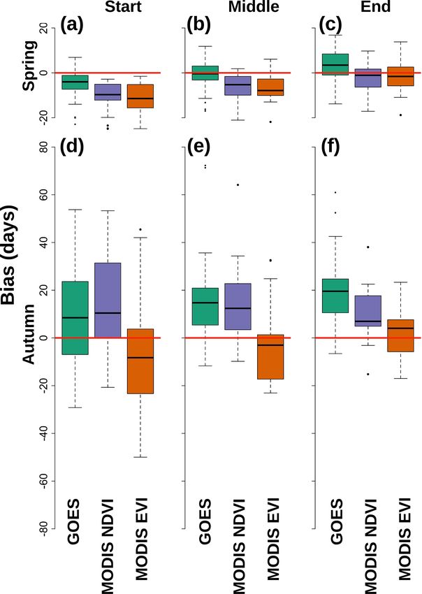
1974                               K. I. Wheeler and M. C. Dietze: Improving the monitoring of deciduous broadleaf phenology

Figure 1. Map of 2016 National Land Cover Database (NLCD) classification (Jin et al., 2019; Yang et al., 2018) for the study region showing
the locations of the selected sites. Selected sites are located throughout the deciduous forested area in the United States. Specific locations
are given in Table 1.

Table 1. Characteristics of selected sites including the coordinates and some climate data from WorldClim (Hijmans et al., 2005), which
were assessed from the PhenoCam website (https://phenocam.sr.unh.edu/webcam/, last access: 1 July 2020).

          Site name                                                            Latitude       Longitude           Mean annual                 Mean annual
                                                                                                               temperature (◦ C)        precipitation (mm)
          Marcell                                                               47.514         −93.469                            2.9               687.0
          Willow Creek                                                          45.806         −90.079                            3.9               820.0
          University of Michigan Biological Station (UMBS)                      45.560         −84.714                            5.9               797.0
          Bartlett                                                              44.065         −71.288                            5.5              1224.0
          Hubbard Brook                                                         43.927         −71.741                            4.6              1190.0
          Harvard Forest                                                        42.538         −72.172                            6.8              1139.0
          Green Ridge                                                           39.691         −78.407                           10.5               935.0
          Morgan Monroe                                                         39.323         −86.413                           11.2              1087.0
          Missouri Ozarks                                                       38.744         −92.200                           12.4               974.0
          Shenandoah                                                            38.617         −78.350                            8.4              1222.0
          Bull Shoals                                                           36.563         −93.067                           13.9              1084.0
          Duke                                                                  35.974         −79.100                           14.6              1166.0
          Shining Rock                                                          35.390         −82.775                            9.3              1835.0
          Coweeta                                                               35.060         −83.428                           12.5              1722.0
          Russell Sage∗                                                         32.457         −91.974                           18.1              1341.0
        ∗ Note: due to the cessation of PhenoCam data collection in 2019, Russell Sage was only included in the 2018 analysis.

Biogeosciences, 18, 1971–1985, 2021                                                                               https://doi.org/10.5194/bg-18-1971-2021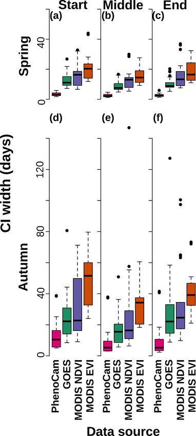
K. I. Wheeler and M. C. Dietze: Improving the monitoring of deciduous broadleaf phenology                                    1975

assessing phenological patterns and not remote sensing qual-       respectively; and k is the change-point day in the summer
ity control algorithms.                                            where the function switches from the green-down logistic
   Because overall atmospheric attenuation and differences         curve to the green-up logistic curve, which we assumed to
in viewing angles between the sites were not corrected for,        be the 182nd day of the year (1 July) in order to separate the
the NDVI values are not exactly equivalent to those mea-           year into two, which has been done elsewhere (e.g., Fu et al.,
sured at the ground. Thus, while we show comparisons across        2016). Spring green-up was completed by the end of June at
days at the same site are possible, we advise further NDVI         all of our sites; thus, the model fits were not heavily sensi-
processing is needed to make comparisons of NDVI values            tive to this assumption. We assumed that the minimum (d)
across sites or use the underlying radiances in radiative trans-   and the maximum (c + d) phenological index values (GCC,
fer models. Transition dates and the seasonal curves for in-       NDVI, EVI) would not change during this 1 year for all sites,
dividual sites should be minimally affected because the view       and, thus, both parts of the change-point function fit the same
angle remains constant within a site, and the processing al-       c and d values. Years were fit independently for each site
gorithm does account for subdaily variability in atmospheric       and, thus, we did not assume that the c and d values were the
attenuation.                                                       same between years. To compare the influence of the differ-
                                                                   ent data sources on the uncertainty in the posterior, we used
2.2.3    MODIS and PhenoCam data download                          relatively uninformative Gaussian priors for the parameters
                                                                   (Table 2), which were created through simulating reasonable
The 250 m 16 d NDVI and EVI bands from the MODIS                   data. Since the motivation for this study was to illustrate the
product MOD13Q1 were used for the study period (Didan,             ability of GOES to monitor phenological change by com-
2015). This product was selected because it is easily accessi-     paring it to other remotely-sensed data sources, we focused
ble through the MODISTools R package (Tuck et al., 2014),          on only one transition date estimation method; though, addi-
and the same temporal resolution for MODIS products has            tional methods are explored elsewhere (e.g., Klosterman et
been used in numerous other comparisons between phenol-            al., 2014).
ogy data sources (e.g., Ahl et al., 2006; Hmimina et al., 2013;       Additionally, since the diurnal fit method (Wheeler and
Richardson et al., 2018b; Zheng and Zhu, 2017). Product            Dietze, 2019) produces estimates of uncertainty on daily
data quality flags were applied to MODIS data. Daily midday        NDVI, the means and precisions were incorporated in a nor-
PhenoCam GCC and standard deviation values were down-              mally distributed errors-in-variable model within the phenol-
loaded directly from the PhenoCam website archive (Pheno-          ogy model. Likewise, errors-in-variable models were applied
Cam, 2018 and 2019; Seyednasrollah et al., 2019). The Phe-         for the PhenoCam sites using the provided daily GCC stan-
noCam at Russell Sage did not collect data for most of 2019,       dard deviation. Since the MOD13Q1 product does not pro-
and, thus, we only fit 1 year of data (2018) to this site.         vide a daily quantification of uncertainty (other than the qual-
                                                                   ity flags that we separately applied), generic values were used
2.3     Phenology model fitting
                                                                   based on the standard deviations given in Miura et al. (2000)
Phenological curves were fit for each source of data (GOES         of 0.01 and 0.02 for NDVI and EVI observations, respec-
NDVI, MODIS NDVI, MODIS EVI, and PhenoCam GCC).                    tively.
Based on the highly cited Zhang et al. (2003) paper, spring           The phenology models were fit in JAGS (Plummer, 2018;
and autumn phenological changes were both modeled using            version 4.3.0) using standard Markov chain Monte Carlo
a logistic curve calculated following Eq. (2):                     (MCMC) approaches. JAGS was called from R (R Core
                                                                   Team, 2017; version 3.4.1) using the rjags (Plummer, 2018;
            c                                                      version 4.7) and runjags (Denwood, 2016) packages. Five
µt =              + d,                                      (2)
        1 + ea+bt                                                  chains were run and all models converged as assessed us-
where t is the time in days, µt is the phenology metric, a         ing Gelman–Brooks–Rubin statistic (GBR 5000 after burn-in was removed.
d is the winter background value for the metric. The inter-        From the posterior outputs, 95 % of CIs were calculated. To
pretation and realistic limits of the parameters a and b are       plot and compare the different data sources, which inherently
somewhat obscure, so we reparametrized the model in terms          have different ranges, the predicted phenological curves for
of the midpoint date (50 % change), M = −a/b. This gives a         all joint parameter posteriors were rescaled to have a range
double-logistic curve calculated following Eq. (3):                of 0 to 1.
      (                                                               As explained in Zhang et al. (2003), the start- and end-of-
                  c
         1+exp[bA (t−MA )] + dt > k                                season transition dates for the double logistic fits were cal-
µt =             c                  ,                     (3)      culated as the roots of the third derivative of Eq. (3), which
         1+exp[bS (t−MS )] + dt ≤ k
                                                                   is illustrated in Fig. 2. The roots of the third derivative of
where bA and bS indicate the b parameters (rate of change)         our reparametrized function (Eq. 3) were calculated follow-
for the autumn green-down and the spring green-up, respec-
tively; MA and MS are the autumn and spring midpoints,

https://doi.org/10.5194/bg-18-1971-2021                                                   Biogeosciences, 18, 1971–1985, 2021
1976 K. I. Wheeler and M. C. Dietze: Improving the monitoring of deciduous broadleaf phenology
Table 2. Parameter priors. “Satellites” refers to all GOES, MODIS NDVI, and MODIS EVI. The priors on when the middle of spring and
autumn occurred were set as the day of year (DOY). Normal distribution is abbreviated with N.
Parameter Parameter Data Distribution
name abbreviation source (mean, standard deviation)
Middle of spring (DOY) MS All N (110, 40)
Middle of autumn (DOY) MA All N (300, 40)
Spring rate of change bS All N (−0.10, 0.05)
Autumn rate of change bA All N (0.10, 0.05)
Minimum of phenological curve d Satellites N (0.6, 0.2)
Minimum of phenological curve d PhenoCam N (0.35, 0.15)
Range of phenological data c Satellites N (0.4, 0.2)
Range of phenological data c PhenoCam N (0.3, 0.15)
ing Eqs. (4) and (5):
√
b × M + log( 3 + 2)
Root1 = , (4)
b
√
b × M + log(2 − 3)
Root2 = , (5)
b
where Root1 signifies the transition dates of the start of sea-
son and end of season for spring and autumn, respectively.
Root2 signifies the end of season and start of season for
spring and autumn, respectively. A total of 95 % of CIs were
calculated from the 50 % midpoint transition date posteriors
and from the sample-specific Root1 and Root2 values.
2.4 Model comparison
Transition dates were compared between the different data
sources with an emphasis on how the transition date esti-
mates from the satellite-based data compared to PhenoCam.
We calculated the coefficient of determination (R 2 ) and root-
mean-square error (RMSE) by comparing the means of the
transition dates from one data source with the means of the
transition dates from another source for all possible combina-
tions. It is important to note that these calculations are based
on the deviation from the one-to-one line and not the line of
best fit, which is often different from the predicted line. Since Figure 2. Schematic based off of Fig. 2 in Zhang et al. (2003) de-
scribing the selection of transition dates (shown using the vertical
we are testing the similarity of the transition date estimates
lines). Panel (a) illustrates an example phenological curve of green-
from the two sources, the predicted line is the one-to-one
down and green-up. Panel (b) illustrates the first derivative. Panel
line. Additionally, bias of the transition dates was assessed (c) illustrates the second derivative where the root (second deriva-
by subtracting samples from the joint parameter posteriors tive equals 0) gives the value of the date of the middle of season.
of one source from those of another source. The medians of Panel (d) illustrates the third derivative where the roots give the
these differences (one median for each site) were then av- start and end of both seasons.
eraged across sites for each comparison. Width of 95 % of
CIs was also compared between the different data sources
for each transition date using paired t tests. 3 Results
3.1 Overall fits
The selected phenological model fit well to the GOES daily
data (Fig. 3a and b, Supplement Figs. S3 and S4). Credible
interval widths in the rescaled phenology fits were notice-
Biogeosciences, 18, 1971–1985, 2021 https://doi.org/10.5194/bg-18-1971-2021K. I. Wheeler and M. C. Dietze: Improving the monitoring of deciduous broadleaf phenology 1977
ably narrower for PhenoCam models than GOES and similar Table 3. Summary statistics for comparisons with PhenoCam tran-
between the two MODIS products (Fig. 3a and b, Supple- sition dates.
ment Figs. S5 and S6). Several sites (e.g., Green Ridge 2018;
Fig. 3e and g) had spring green-up periods that were shorter Data source R2 RMSE (days) Average bias∗
than the 16 d temporal resolution of the MODIS products (days; 95 % CI)
but were shown in the GOES measurements (Fig. 3e). Based Start of spring
on the output from the paired t tests, PhenoCam transition
GOES 0.62 9.06 −5.18 ± 0.03
date uncertainties were statistically narrower than those of
MODIS NDVI 0.00 13.53 −10.18 ± 0.1
all satellite data for all transition dates (p value < 0.015 for MODIS EVI 0.00 13.4 −11.66 ± 0.03
all comparisons; Table S2). All GOES transition dates were
statistically more certain (based on CI width) than the corre- Middle of spring
sponding MODIS EVI estimates (p value < 0.03) but were GOES 0.77 7.06 −0.92 ± 0.03
only significantly more certain than MODIS NDVI for the MODIS NDVI 0.00 10.86 −5.56 ± 0.04
middle and end of spring (Fig. 4; Supplement Table S2). MODIS EVI 0.5 9.42 −6.61 ± 0.03
End of spring
3.2 Spring transition dates
GOES 0.71 7.99 3.35 ± 0.03
GOES was correlated with PhenoCam for the start of spring MODIS NDVI 0.12 10.49 −0.95 ± 0.1
transition, where MODIS possessed an early bias (Fig. 5; Ta- MODIS EVI 0.71 7.7 −1.57 ± 0.03
ble 3). GOES vs. PhenoCam (i.e., PhenoCam median tran- Start of autumn
sition dates were the independent variable and GOES me-
GOES 0.00 32.3 12.59 ± 0.11
dian transition dates were the dependent variable) had the
MODIS NDVI 0.00 34.2 17.84 ± 0.26
highest R 2 values (0.62 versus 0.00 and 0.00) and the lowest
MODIS EVI 0.00 26.67 −7.5 ± 0.11
RMSE and average bias (5.18 ± 0.03 earlier than PhenoCam;
Table 3). Both MODIS NDVI and EVI, on the other hand, Middle of autumn
were biased earlier by 10.18 ± 0.1 and 11.66 ± 0.03 d on av- GOES 0.00 25.61 17.04 ± 0.07
erage, respectively. This bias was consistent amongst most MODIS NDVI 0.00 23.43 14.16 ± 0.08
sites (Fig. 6a). GOES was also most correlated with Pheno- MODIS EVI 0.00 15.64 −2.7 ± 0.07
Cam for the estimate of the middle of spring, with the high-
End of autumn
est R 2 value (0.72), lowest RMSE (7.06 d), and lowest aver-
age bias of 0.92 ± 0.03 d earlier than PhenoCam (Table 3). GOES 0.00 26.58 21.5 ± 0.07
Most of the MODIS NDVI and EVI models were biased MODIS NDVI 0.00 16.17 10.47 ± 0.24
early (Fig. 6b). Both MODIS data products were slightly MODIS EVI 0.36 11.23 2.11 ± 0.06
more correlated with PhenoCam for the end of spring than ∗ Negative indicates the data source is earlier than PhenoCam. The widths of
GOES. MODIS NDVI had the highest R 2 value of 0.80 but the 95 % credible intervals (CIs) of the biases are given.
had a slightly earlier bias than MODIS EVI (1.75 ± 0.04 d
vs. 0.79 ± 0.05 d). MODIS EVI and GOES had the same R 2
values of 0.71, but GOES had a later bias of 3.35 ± 0.03 d NDVI and GOES for the first two transition dates (GOES
(Table 3). There existed less correlation between GOES and was 5.25 ± 0.24 d earlier and 2.89 ± 0.05 d later than MODIS
the MODIS products (Supplement Table S3). NDVI in the start and middle of autumn, respectively; Sup-
plement Table S3).
3.3 Autumn transition dates
4 Discussion
Autumn transition dates agreed less across all sources of data
than in spring. Except for MODIS EVI at the end of autumn 4.1 Spring transition date similarity
(R 2 of 0.36), none of the satellite-based data sources ex-
plained any variation in PhenoCam transition date estimates Our hypothesis that GOES spring transition dates are more
(Table 3). Both NDVI sources (i.e., GOES and MODIS) were similar than MODIS to PhenoCam ones was supported by
consistently biased later (Table 3). MODIS EVI was biased our results for the start and middle of spring. While the
earlier than PhenoCam for the transition dates of the begin- MODIS earlier sensing start of spring compared to Pheno-
ning and middle of autumn. Except for the middle of autumn Cam has also been attributed to a variety of reasons ranging
where MODIS NDVI and GOES had a slight correlation (R 2 from different viewing angles that sense the heterogeneity of
of 0.34), satellite data sources were overall uncorrelated with phenological change between different canopy layers (Ahl
each other for all autumn transition dates (all had R 2 val- et al., 2006; Richardson and O’Keefe, 2009; Keenan et al.,
ues = 0.00). The biases were the smallest between MODIS 2014b; Ryu et al., 2014; Schwartz et al., 2002), spatial scal-
https://doi.org/10.5194/bg-18-1971-2021 Biogeosciences, 18, 1971–1985, 20211978 K. I. Wheeler and M. C. Dietze: Improving the monitoring of deciduous broadleaf phenology
Figure 3. Time series of data from GOES NDVI daily data (a, b), PhenoCam GCC (c, d), MODIS NDVI (e, f), MODIS EVI (g, h), and
the rescaled credible intervals (i, j) for Green Ridge 2018 (left column) and Harvard Forest 2019 (right column). (a–h) Mean observations
in black dots with 95 % confidence intervals shown with vertical gray lines. The 95 % credible intervals (CIs) are given with the different
shading specific to each data source. The Green Ridge 2018 spring occurred more quickly than the MODIS temporal resolution but was
captured by the daily resolution of the GOES data.
ing affected by significant topography (Fisher et al., 2007), Contrary to our hypothesis, though, we found that both
snowmelt (Delbart et al., 2006), all these issues should af- MODIS indices were slightly less biased than GOES with
fect the GOES–PhenoCam comparison as well. Based off PhenoCam at the end of spring, even with a R 2 value higher
of the similarity found here between GOES and Pheno- than or similar to MODIS NDVI and EVI, respectively. Bias
Cam at marking the start and middle of spring, the mis- is likely more reliable as a measure of similarity than R 2 and
match between MODIS and PhenoCam is likely largely due RMSE because it includes the uncertainties in the transition
to the temporal resolution of the MODIS products. Hufkens dates for each site by utilizing the MCMC posterior sam-
et al. (2012) also point out that the temporal resolution of ples instead of just comparing the median transition dates
MODIS products cannot be expected to precisely track rapid for each site. The later bias of GOES compared to Phe-
leaf emergence in the spring due to the longer temporal noCam and the MODIS products could potentially be due
resolution. By averaging over a relatively long time period to an early bias in both PhenoCam and the MODIS prod-
(compared to the length of spring green-up), such techniques ucts. PhenoCam GCC has been found previously to reach its
likely prematurely inflate NDVI and EVI values, giving the end of spring before many physiological traits such as to-
false impression that green-up occurred earlier. GOES, on tal chlorophyll concentrations, leaf area and mass, leaf nitro-
the other hand, allows for daily NDVI estimates that are in- gen and carbon concentrations, and leaf area index (Keenan
herently more capable of tracking the initial spring increase. et al., 2014b; Yang et al., 2014). Thus, inherent differences
between GCC and NDVI could cause the slightly later bias
Biogeosciences, 18, 1971–1985, 2021 https://doi.org/10.5194/bg-18-1971-2021K. I. Wheeler and M. C. Dietze: Improving the monitoring of deciduous broadleaf phenology 1979
their study was to investigate the impacts of land-cover het-
erogeneity on transition date comparisons between different
sources, and, thus, they included more heterogeneous land-
scapes in their dataset. They concluded that due to scaling
issues, MODIS pixels that have smaller proportions of de-
ciduous forests have MODIS end-of-spring estimates that are
later than near-surface estimates. Thus, it is reasonable to
assume that our attempt to not include any sites with sub-
stantial non-forest land-cover types within the MODIS and
GOES pixels would lower our average bias. The effects of
land-cover heterogeneity on the estimates of end-of-spring
transition should be kept in mind when using GOES to mon-
itor more heterogeneous sites.
As with many studies, the results and conclusions of this
study could depend on the methods used. It is possible that
a different transition date estimation method (e.g., the one
proposed by Klosterman et al., 2014, that also accounted for
summer green-down, which we were not focused on) would
result in different conclusions. If there is bias in the meth-
ods here to estimate transition dates, it is shared across data
sources, sites, and years. Similarly, using a different MODIS
product might also result in different conclusions. While a
daily MODIS product does exist, it is also created using
multi-day periods of measurements (Ju et al., 2010) and,
thus, is also possibly subject to similar constraints. We en-
courage others to consider more complex models and other
phenology products, but the primary aim of this study is to
demonstrate the value of GOES for studying phenology with
an initial comparison to PhenoCams and MODIS.
4.2 Spring and autumn compared
As we hypothesized, spring transition dates were more simi-
lar across data sources than autumn ones. This mismatch be-
tween PhenoCam GCC autumn transition dates and NDVI
and EVI (low R 2 values and high biases) has been found in
numerous other studies (e.g., Hufkens et al., 2012; Keenan et
al., 2014a; Klosterman et al., 2014; Richardson et al., 2018b;
Figure 4. The 95 % credible interval (CI) widths for the different Zhang et al., 2018). This is most likely due to physiological
data sources for spring start (a), middle (b), and end (c) and autumn differences between the different metrics (i.e., GCC, NDVI,
start (d), middle (e), and end (f). Colors denote the different data and EVI) that become more apparent in the autumn, with
sources, which are labeled on the x axis. PhenoCam had the most changes in color and canopy structure often occurring sepa-
certain transition date estimates, and GOES was always more cer-
rately. While all three metrics measure some combination of
tain than MODIS EVI but only more certain than MODIS NDVI for
the middle and end of spring.
greenness and canopy structure, only GCC directly considers
green reflectance in its calculation; leaf presence and canopy
structure (Kobayashi et al., 2007; Pettorelli et al., 2005) have
been found to impact NDVI and EVI more. The higher un-
of GOES compared to PhenoCam at the end of spring. This certainties in the autumn transition dates, compared to spring
should not affect GOES’s ability to monitor interannual vari- ones, across all data sources were expected given the longer
ability in this transition date as more years become avail- season length and the higher heterogeneity in autumn com-
able. MODIS could be biased early for the end of spring pared to spring. For example, triggers of autumn phenology
in a similar way as that discussed in the previous paragraph are less understood and consistent than spring (Piao et al.,
related to its temporal resolution. Klosterman et al. (2014) 2019), and the timing of autumn phenological events differs
found, however, that on average MODIS had a later end-of- more greatly between species than in spring (Richardson et
spring estimate than PhenoCam. One primary component of al., 2006). Like the other data sources, GOES spring tran-
https://doi.org/10.5194/bg-18-1971-2021 Biogeosciences, 18, 1971–1985, 20211980 K. I. Wheeler and M. C. Dietze: Improving the monitoring of deciduous broadleaf phenology
Figure 5. Scatter plots showing how the different data sources compare for their estimation of spring start (a), middle (b), and end (c) and
autumn start (d), middle (e), and end (f). Median transition dates are indicated by the point, and 95 % credible intervals are indicated by the
lines. The x axis gives the day of year of the PhenoCam (PC) transition and the y axis indicates the day of year of the different satellite data
sources, which are color-coded as indicated in the legend. Spring correlations are much higher than autumn ones, and GOES dates are more
correlated at the start and middle of spring (a, b) but are slightly biased late at the end of spring (c).
sition date estimates were most certain and most similar to ing daily NDVI values that change seasonally would also im-
those derived from other data sources. prove the ability to estimate winter NDVI values with more
certainty. These will likely help improve the correlation be-
4.3 Autumn transition date similarity tween GOES NDVI and MODIS NDVI.
We hypothesized that in the autumn, the transition dates 4.4 Uncertainty in transition date estimates
derived from GOES NDVI data are most similar to those
from MODIS NDVI data, which was mostly true. The low We hypothesized that the increased temporal frequency in
biases that existed between the two at the start and mid- GOES data would produce more certain estimates of tran-
dle of autumn (MODIS NDVI was 5.25 ± 0.24 d later and sition dates than MODIS. In practice, we found differences
2.89 ± 0.05 d earlier than GOES, respectively; Supplement between MODIS indices, with GOES transition dates being
Table S3) are promising while the high end-of-autumn bias significantly more certain than MODIS EVI for all transi-
(MODIS NDVI was 11.03 ± 0.24 d earlier than GOES) could tion dates but only significantly more certain than MODIS
potentially be due to the high amount of noise in the GOES NDVI for the start and middle of spring. However, as pre-
data that remains in the winter at many sites (Supplement viously discussed, there are nontrivial differences between
Figs. S2 and S3). Future directions for GOES that should what NDVI and GCC are measuring in the autumn and end
help decrease these biases include developing a snow cover of spring that transcend simple issues of data quality and
mask (which is a planned GOES product), developing a more quantity, which suggests GOES is providing important new
sophisticated atmospheric correction algorithm for GOES information about vegetation phenology. Once future work
reflectance data, and developing methodology for correct- further improves the GOES products, reducing noise due to
ing for seasonal variations in solar angle. GOES will inher- factors such as snow and atmospheric attenuation, the widths
ently be better at establishing a winter baseline at sites with of the CIs are expected to improve. Additionally, the lack
less snowy days than sites that consistently have a layer of of a spatially and temporally varying MODIS uncertainty
snow obstructing accurate satellite measurements. Develop- product, as we have produced for GOES, provided a limi-
ing multi-year phenology models to increase the number of tation to this comparison, and it is possible that specific daily
winter observations by assuming the winter NDVI baseline MODIS uncertainties, congruent to that we used from the
is similar between years would improve this. Furthermore, GOES data, would affect this conclusion. In particular, many
more informative priors in the diurnal fit model for estimat- of the MODIS validation efforts have focused on within-
Biogeosciences, 18, 1971–1985, 2021 https://doi.org/10.5194/bg-18-1971-2021K. I. Wheeler and M. C. Dietze: Improving the monitoring of deciduous broadleaf phenology 1981
4.5 Future phenological applications of GOES NDVI
data
With its full coverage and high temporal resolution, GOES-
16 and GOES-17 have the potential to revolutionize the study
of leaf phenology and allow for a variety of studies that pre-
viously would not have been possible at the extent they are
now. First, many studies have found that climate change is
altering phenology on the scale of days per decade (Cleland
et al., 2007; Keenan et al., 2014a; Parmesan and Yohe, 2003;
Root et al., 2003). The long temporal scale of the studied
MODIS NDVI and EVI products limits their ability to pre-
cisely and accurately monitor both these trends and interan-
nual variability. While a daily MODIS NDVI product is be-
coming more readily available (and MODIS measurements
are taken sub-daily, but at varying viewing angles), it still re-
mains more inaccessible than many of the lower-frequency
MODIS data products because it is relatively new. It is im-
portant to have additional remotely sensed data sources, es-
pecially ones that are not affected by changing viewing an-
gles.
Second, GOES provides real-time data of spring green-up
even for those springs that occur quicker than the 16 d res-
olution of this MODIS product (e.g., Green Ridge 2018 in
Fig. 3). These sites possessed no 16 d MODIS NDVI nor EVI
measurements during the green-up period. This limitation
would become even more severe when monitoring green-up
in real time, as the transition would only be detected after
the fact. The seasonal curve fitting methodology used here to
Figure 6. The different biases for the different satellite-based data estimate transition dates is not suitable in real time, but alter-
sources compared to PhenoCam for their estimation of spring start
native methods, such as determining that spring has started
(a), middle (b), and end (c) and autumn start (d), middle (e), and
if the phenological index is 10 % greater than the winter
end (f). A negative bias indicates the given data source was earlier
than PhenoCam. The red line denotes zero bias. Boxes are color baseline or iteratively assimilating data into a process model
coded by the data source as indicated on the x axis. The biases are (Viskari et al., 2015), could be used to provide insight into
larger in the autumn than in the spring. There are some with little whether or not certain transition dates have occurred in real
median bias. time. With the data that GOES supplies, it becomes more
possible to monitor and forecast the start and progression of
green-up at large scales using near-real-time data, instead of
season comparisons (e.g., Miura et al., 2000) not periods having to wait for the next reliable MODIS product value,
of phenological transition, and, thus, MODIS uncertainties which might be 15 d away.
are likely underestimated. Furthermore, the differences in re- A third beneficial future application of the high-temporal-
sults between comparing GOES transition dates’ CI widths resolution GOES NDVI data is the ability to monitor the
to those from MODIS NDVI and EVI are likely partially effects of storms (e.g., hurricanes), droughts, and frosts on
due to the differences in observational error applied. Based phenology and NDVI. It is possible that the effects of some
on Miura et al. (2000), a smaller observational error was ap- of these disturbances are only present for less than the tem-
plied to MODIS NDVI than MODIS EVI, which likely was poral resolution of MODIS. For example, Richardson et
enough to make all GOES transition date estimates signif- al. (2018b) found that the effect of a spring frost event
icantly more certain than the respective MODIS EVI esti- was visible within PhenoCam data but not clearly visible
mates, but not always MODIS NDVI. This emphasizes the within the 16 d MODIS data. By providing higher-temporal-
importance of providing uncertainty estimates with remotely resolution spring NDVI data, it is more likely that the effects
sensed phenology data, which fitting diurnal curves to GOES of similar frost events could be observed at more areas that
data provides (Wheeler and Dietze, 2019). do not have a PhenoCam present.
A fourth benefit is that by combining data from multi-
ple high-temporal-resolution sources (i.e., PhenoCam and
GOES), we may now ask questions related to differentiat-
https://doi.org/10.5194/bg-18-1971-2021 Biogeosciences, 18, 1971–1985, 20211982 K. I. Wheeler and M. C. Dietze: Improving the monitoring of deciduous broadleaf phenology
ing the physiological impacts of phenological change in dif- Acknowledgements. This work was made possible by the U.S. Na-
ferent indices and at different spatial scales. For example, tional Science Foundation grant 1638577. KIW also acknowledges
with high-temporal-resolution NDVI data, we can now start support under the U.S. National Science Foundation Graduate Re-
asking questions about what specific phenological processes search Fellowship grant number 1247312. Special thanks are due
control the rate of spring increase (i.e., budburst vs. leaf ex- to the Dietze lab members for feedback on the manuscript. We
thank our many collaborators, including site principal investiga-
pansion) and how these are affected by spatial scale. Simi-
tors and technicians, for their efforts in support of PhenoCam. The
larly, combining PhenoCam and GOES data has the potential development of PhenoCam has been funded by the Northeastern
to help us better disentangle different autumn phenological States Research Cooperative, NSF’s Macrosystems Biology pro-
processes (i.e., leaf color change vs. leaf fall). gram (awards EF-1065029 and EF-1702697), and DOE’s Regional
We are not suggesting that GOES should replace other and Global Climate Modeling program (award DE-SC0016011).
phenology data sources but rather that a combination of dif- We acknowledge additional support from the US National Park
ferent data sources, which each have their own strengths and Service Inventory and Monitoring Program and the US National
weaknesses, is beneficial. MODIS has a much longer record Phenology Network (grant number G10AP00129 from the United
of data than GOES and still remains an important source of States Geological Survey) and from the US National Phenology
information. Additionally, it has a different spatial scale that Network and North Central Climate Science Center (cooperative
is between PhenoCam and GOES, and a combination of the agreement number G16AC00224 from the United States Geologi-
cal Survey). We also thank the USDA Forest Service Air Resource
three could help answer spatial questions related to NDVI
Management program and the National Park Service Air Resources
(e.g., how does NDVI scale between canopy level and land- program for contributing their camera imagery to the PhenoCam
scape level and how does this change seasonally?). archive. Research at the Bartlett Experimental Forest tower is sup-
In conclusion, we have shown that GOES-16 and GOES- ported by the National Science Foundation (grant DEB-1114804)
17 possess great potential at enhancing the monitoring of leaf and the USDA Forest Service’s Northern Research Station. Re-
phenology, which will allow us to ask and answer new ques- search at the Coweeta flux tower is funded through the USDA Forest
tions and improve our knowledge of this complicated but im- Service, Southern Research Station; USDA Agriculture and Food
portant aspect of ecology and environmental science. Research Initiative Foundational program, award number 2012-
67019-19484; EPA agreement number 13-IA-11330140-044; and
the National Science Foundation, Long Term Ecological Research
Code availability. All code is available on GitHub at (LTER) program, award no. DEB-0823293. Research at Harvard
https://github.com/k-wheeler/NEFI_pheno/tree/master/GOES_ Forest is partially supported through the National Science Founda-
PhenologyPaper_Code (last access: 17 January 2021) tion’s LTER program (DEB-1237491) and Department of Energy
(see the main file GOES_Phenology_Paper_Code.Rmd) Office of Science (BER). The Hubbard Brook Ecosystem Study
and https://github.com/k-wheeler/NEFI_pheno/tree/master/ is a collaborative effort at the Hubbard Brook Experimental For-
PhenologyBayesModeling (last access: 17 January 2021) est, which is operated and maintained by the USDA Forest Ser-
(https://doi.org/10.5281/zenodo.4589080, Wheeler and Dietze, vice, Northern Research Station, Newtown Square, PA. Research
2021). at the MOFLUX site is supported by the U.S. Department of En-
ergy, Office of Science, Office of Biological and Environmental
Research program, Climate and Environmental Sciences Division.
ORNL is managed by UT-Battelle, LLC, for the U.S. Department
Data availability. All data were publicly available and can be ac-
of Energy under contract DE-AC05-00OR22725. U.S. Department
cessed as described in the Methods section.
of Energy support for the University of Missouri (grant DE-FG02-
03ER63683) is gratefully acknowledged. Research at the Morgan-
Monroe AmeriFlux site is supported by the U.S. Department of En-
Supplement. The supplement related to this article is available on- ergy, Office of Science, Office of Biological and Environmental Re-
line at: https://doi.org/10.5194/bg-18-1971-2021-supplement. search through the AmeriFlux Management Project administered
by Lawrence Berkeley National Lab. Funding for the Shenandoah
PhenoCam and related research has been provided by the U.S. Ge-
Author contributions. KIW and MCD designed the study, and KIW ological Survey Land Change Science Program (Shenandoah Na-
executed the modeling and analysis. KIW wrote the manuscript with tional Park Phenology Project) with logistical support from the Na-
input and suggestions from MCD throughout the writing process. tional Park Service in collaboration with the University of Virginia
Department of Environmental Sciences. Camera images from the
Shining Rock Wilderness are provided courtesy of the USDA For-
Competing interests. The authors declare that they have no conflict est Service Air Resources Management Program. Primary support
of interest. for the University of Michigan AmeriFlux Core Site (US-UMd) was
provided by the Department of Energy Office of Science. Infrastruc-
ture support was provided by the University of Michigan Biologi-
Disclaimer. Any opinion, findings, and conclusions or recommen- cal Station. Research at the Willow Creek AmeriFlux core site is
dations expressed in this material are those of the authors and do not provided by the Dept. of Energy Office of Science to the ChEAS
necessarily reflect the views of the National Science Foundation. Cluster.
Biogeosciences, 18, 1971–1985, 2021 https://doi.org/10.5194/bg-18-1971-2021K. I. Wheeler and M. C. Dietze: Improving the monitoring of deciduous broadleaf phenology 1983
Financial support. This research has been supported by the Na- meta-analysis of autumn phenology studies, Ann. Bot.-London,
tional Science Foundation (grant nos. 1638577 and 1247312). 116, 875–888, https://doi.org/10.1093/aob/mcv055, 2015.
GOES-R Algorithm Working Group and GOES-R Series Program:
NOAA GOES-R Series Advanced Baseline Imager (ABI) Level
Review statement. This paper was edited by Paul Stoy and re- 2 Clear Sky Mask, NOAA National Centers for Environmental
viewed by three anonymous referees. Information, https://doi.org/10.7289/V5SF2TGP, 2018.
GOES-R Calibration Working Group and GOES-R Series
Program: NOAA GOES-R Series Advanced Baseline Im-
ager (ABI) Level 1b Radiances. [Channels 2 and 3],
NOAA National Centers for Environmental Information,
References https://doi.org/10.7289/V5BV7DSR, 2017.
Hijmans, R. J., Cameron, S. E., Parra, J. L., Jones, P. G.,
Ahl, D. E., Gower, S. T., Burrows, S. N., Shabanov, N. V., Myneni, and Jarvis, A.: Very high resolution interpolated climate sur-
R. B., and Knyazikhin, Y.: Monitoring spring canopy phenol- faces for global land areas, Int. J. Climatol., 25, 1965–1978,
ogy of a deciduous broadleaf forest using MODIS, Remote Sens. https://doi.org/10.1002/joc.1276, 2005.
Environ., 104, 88–95, https://doi.org/10.1016/j.rse.2006.05.003, Hmimina, G., Dufrêne, E., Pontailler, J.-Y., Delpierre, N., Aubi-
2006. net, M., Caquet, B., de Grandcourt, A., Burban, B., Flechard,
Alekseychik, P. K., Korrensalo, A., Mammarella, I., Vesala, T., C., Granier, A., Gross, P., Heinesch, B., Longdoz, B., Moureaux,
and Tuittila, E.-S.: Relationship between aerodynamic rough- C., Ourcival, J.-M., Rambal, S., Saint André, L., and Soudani,
ness length and bulk sedge leaf area index in a mixed-species K.: Evaluation of the potential of MODIS satellite data to predict
boreal mire complex, Geophys. Res. Lett., 44, 5836–5843, vegetation phenology in different biomes: An investigation using
https://doi.org/10.1002/2017GL073884, 2017. ground-based NDVI measurements, Remote Sens. Environ., 132,
Cleland, E., Chuine, I., Menzel, A., Mooney, H., and 145–158, https://doi.org/10.1016/j.rse.2013.01.010, 2013.
Schwartz, M.: Shifting plant phenology in response Hudson, J. E., Levia, D. F., Wheeler, K. I., Winters, C. G.,
to global change, Trends Ecol. Evol., 22, 357–365, Vaughan, M. C. H., Chace, J. F. and Sleeper, R.: Ameri-
https://doi.org/10.1016/j.tree.2007.04.003, 2007. can beech leaf-litter leachate chemistry: Effects of geogra-
Delbart, N., Le Toan, T., Kergoat, L., and Fedotova, V.: Re- phy and phenophase, J. Plant Nutr. Soil Sc., 181, 287–295,
mote sensing of spring phenology in boreal regions: A free https://doi.org/10.1002/jpln.201700074, 2018.
of snow-effect method using NOAA-AVHRR and SPOT- Hufkens, K., Friedl, M., Sonnentag, O., Braswell, B. H., Mil-
VGT data (1982–2004), Remote Sens. Environ., 101, 52–62, liman, T., and Richardson, A. D.: Linking near-surface and
https://doi.org/10.1016/j.rse.2005.11.012, 2006. satellite remote sensing measurements of deciduous broadleaf
Denwood, M. J.: runjags: An R Package Providing Interface Util- forest phenology, Remote Sens. Environ., 117, 307–321,
ities, Model Templates, Parallel Computing Methods and Addi- https://doi.org/10.1016/j.rse.2011.10.006, 2012.
tional Distributions for MCMC Models in JAGS, J. Stat. Softw., Jin, S., Homer, C., Yang, L., Danielson, P., Dewitz, J., Li, C., Zhu,
71, 1–25, https://doi.org/10.18637/jss.v071.i09, 2016. Z., Xian, G., and Howard, D.: Overall Methodology Design for
Didan K.: MOD13Q1 MODIS/Terra Vegetation Indices the United States National Land Cover Database 2016 Products,
16-Day L3 Global 250m SIN Grid V006 NDVI and Remote Sens., 11, 2971, https://doi.org/10.3390/rs11242971,
pixel_reliability, NASA EOSDIS Land Processes DAAC, 2019.
https://doi.org/10.5067/MODIS/MOD13Q1.006, 2015. Ju, J., Roy, D. P., Shuai, Y., and Schaaf, C.: Development of
Filippa, G., Cremonese, E., Migliavacca, M., Galvagno, M., Son- an approach for generation of temporally complete daily nadir
nentag, O., Humphreys, E., Hufkens, K., Ryu, Y., Verfaillie, J., MODIS reflectance time series, Remote Sens. Environ., 114, 1–
Morra di Cella, U., and Richardson, A. D.: NDVI derived from 20, https://doi.org/10.1016/j.rse.2009.05.022, 2010.
near-infrared-enabled digital cameras: Applicability across dif- Keenan, T. F., Gray, J., Friedl, M. A., Toomey, M., Bohrer,
ferent plant functional types, Agr. Forest Meteorol., 249, 275– G., Hollinger, D. Y., Munger, J. W., O’Keefe, J., Schmid, H.
285, https://doi.org/10.1016/j.agrformet.2017.11.003, 2018. P., Wing, I. S., Yang, B., and Richardson, A. D.: Net car-
Fisher, J. I., Richardson, A. D., and Mustard, J. F.: Phenology bon uptake has increased through warming-induced changes in
model from surface meteorology does not capture satellite- temperate forest phenology, Nat. Clim. Change, 4, 598–604,
based greenup estimations, Glob. Change Biol., 13, 707–721, https://doi.org/10.1038/nclimate2253, 2014a.
https://doi.org/10.1111/j.1365-2486.2006.01311.x, 2007. Keenan, T. F., Darby, B., Felts, E., Sonnentag, O., Friedl, M.
Fu, Y., Zheng, Z., Shi, H., and Xiao, R.: A Novel Large-Scale A., Hufkens, K., O’Keefe, J., Klosterman, S., Munger, J. W.,
Temperature Dominated Model for Predicting the End of the Toomey, M., and Richardson, A. D.: Tracking forest phe-
Growing Season, edited by W. Yuan, Plos One, 11, e0167302, nology and seasonal physiology using digital repeat pho-
https://doi.org/10.1371/journal.pone.0167302, 2016. tography: a critical assessment, Ecol. Appl., 24, 1478–1489,
Gao, M., Piao, S., Chen, A., Yang, H., Liu, Q., Fu, Y. H. and https://doi.org/10.1890/13-0652.1, 2014b.
Janssens, I. A.: Divergent changes in the elevational gradient of Killingbeck, K. T.: Nutrient Resorption, in: Plant Cell Death Pro-
vegetation activities over the last 30 years, Nat. Commun., 10, cesses, Elsevier, London., 2004.
2970, https://doi.org/10.1038/s41467-019-11035-w, 2019. Klosterman, S. T., Hufkens, K., Gray, J. M., Melaas, E., Son-
Gill, A. L., Gallinat, A. S., Sanders-DeMott, R., Rigden, A. J., Gi- nentag, O., Lavine, I., Mitchell, L., Norman, R., Friedl,
anotti, D. J. S., Mantooth, J. A. and Templer, P. H.: Changes M. A., and Richardson, A. D.: Evaluating remote sens-
in autumn senescence in northern hemisphere deciduous trees: a
https://doi.org/10.5194/bg-18-1971-2021 Biogeosciences, 18, 1971–1985, 2021You can also read