Using a calibrated upper living position of marine biota to calculate coseismic uplift: a case study of the 2016 Kaik oura earthquake, New ...
←
→
Page content transcription
If your browser does not render page correctly, please read the page content below
Earth Surf. Dynam., 8, 351–366, 2020
https://doi.org/10.5194/esurf-8-351-2020
© Author(s) 2020. This work is distributed under
the Creative Commons Attribution 4.0 License.

        Using a calibrated upper living position of marine biota
              to calculate coseismic uplift: a case study
            of the 2016 Kaikōura earthquake, New Zealand
             Catherine Reid1 , John Begg2 , Vasiliki Mouslopoulou3,4 , Onno Oncken4 , Andrew Nicol1 , and
                                               Sofia-Katerina Kufner4,5
                               1 School  of Earth and Environment, University of Canterbury,
                                    Private Bag 4800, Christchurch, 8140, New Zealand
                                2 GNS Science, P.O. Box 30-368, Lower Hutt, New Zealand
            3 National Observatory of Athens, Institute of Geodynamics, Lofos Nimfon, Athens, 11810, Greece
                       4 GFZ Helmholtz Centre Potsdam, German Research Centre for Geosciences,

                                          Telegrafenberg, 14473 Potsdam, Germany
                     5 British Antarctic Survey, High Cross, Madingley Rd, Cambridge, CB3 0ET, UK

                        Correspondence: Vasiliki Mouslopoulou (vasiliki.mouslopoulou@noa.gr)

                                 Received: 30 August 2019 – Discussion started: 9 October 2019
                           Revised: 19 March 2020 – Accepted: 15 April 2020 – Published: 8 May 2020

      Abstract. The 2016 Mw = 7.8 Kaikōura earthquake (South Island, New Zealand) caused widespread complex
      ground deformation, including significant coastal uplift of rocky shorelines. This coastal deformation is used here
      to develop a new methodology, in which the upper living limits of intertidal marine biota have been calibrated
      against tide-gauge records to quantitatively constrain pre-deformation biota living position relative to sea level.
      This living position is then applied to measure coseismic uplift at three other locations along the Kaikōura coast.
      We then assess how coseismic uplift derived using this calibrated biological method compares to that measured
      using other methods, such as light detection and ranging (lidar) and strong-motion data, as well as non-calibrated
      biological methods at the same localities. The results show that where biological data are collected by a real-
      time kinematic (RTK) global navigation satellite system (GNSS) in sheltered locations, this new tide-gauge
      calibration method estimates tectonic uplift with an accuracy of ± ≤ 0.07 m in the vicinity of the tide gauge
      and an overall mean accuracy of ±0.10 m or 10 % compared to differential lidar methods for all locations.
      Sites exposed to high wave wash, or data collected by tape measure, are more likely to show higher uplift
      results. Tectonic uplift estimates derived using predictive tidal charts produce overall higher uplift estimates in
      comparison to tide-gauge-calibrated and instrumental methods, with mean uplift results 0.21 m or 20 % higher
      than lidar results. This low-tech methodology can, however, produce uplift results that are broadly consistent
      with instrumental methodologies and may be applied with confidence in remote locations where lidar or local
      tide-gauge measurements are not available.

Published by Copernicus Publications on behalf of the European Geosciences Union.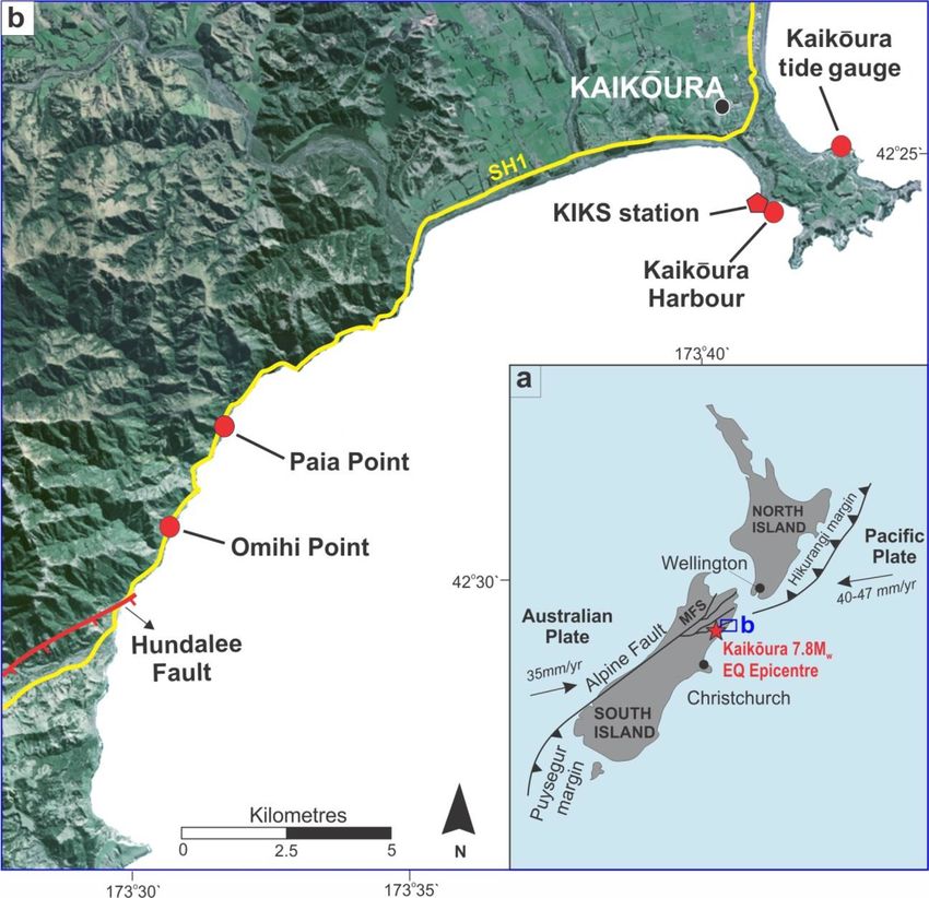
352                       C. Reid et al.: Using a calibrated upper living position of marine biota to calculate coseismic uplift

1   Introduction                                                    marker horizons near a local tide-gauge site. This calibrated
                                                                    information can then be applied to estimating coastal uplift
Vertical displacement has been measured globally using              or subsidence at other sites in the Kaikōura region. Capi-
intertidal marine biota on rocky coastlines, which often            talising on the long-term, continuous, high-precision tide-
provide important constraints for incremental uplift during         gauge readings at Kaikōura Peninsula, biological markers
large-magnitude earthquakes and cumulative geological up-           within the intertidal zone uplifted during the earthquake are
lift (e.g. Alaska: Plafker, 1965; California: Carver et al.,        here utilised to (a) develop a new methodology with which
1994; Mexico: Bodin and Klinger, 1986; Ramirez-Herrera              to independently calculate (and thus calibrate) the upper
and Orozco, 2002; Costa Rica: Plafker and Ward, 1992;               living position of individual intertidal (algal) taxa (organ-
Chile: Fitzroy, 1839; Castilla, 1988; Castilla et al., 2010;        isms which are widely used to measure coseismic vertical
Farías, 2010; Vargas et al., 2011; Melnick et al., 2012; Ar-        displacement) and (b) compare, at each of three localities,
gentina: Ortlieb et al., 1996; eastern Mediterranean: Piraz-        the conventional biologically constrained handheld measure-
zoli et al., 1982; Stiros et al., 1992; Laborel and Laborel-        ments of coseismic uplift to values derived using various
Dugeun, 1994; Mouslopoulou et al., 2015a; Japan: Pirazzoli          real-time remote sensing and other instrumental techniques,
et al., 1985; New Zealand: Mouslopoulou et al., 2019). Bi-          such as RTK GNSS, lidar and strong-motion seismometers.
ological data were the basis for the first written records of       The results may have applications to inform future studies of
coastal uplift following earthquakes along the Chilean coast        the reliability of biological uplift measurements along rocky
(Graham, 1824; Fitzroy, 1839; Wesson, 2017) and continue            shores arising from large earthquakes at mid-latitudes (par-
to provide important constraints for elastic rebound and co-        ticularly in the Southern Hemisphere) and with moderate
seismic slip processes together with the locations, depth and       tidal ranges (e.g. ∼ 2 m), especially where instrumental tech-
dip of causal faults (e.g. Melnick et al., 2012; Wesson et al.,     nologies, such as differential lidar, are not available.
2015; Mouslopoulou et al., 2015b, 2019).
   Biological indicators such as lithophagid borings and
                                                                    2     Geological and biological setting
stranded bioconstructions of corals, coralline algae and bar-
nacles, along with brown algae, gastropods, bivalves and ad-        2.1    The 2016 Kaikōura earthquake
ditional intertidal species with locally reliable tidal elevation
zones, have been used to estimate eustatic sea level changes        The 2016 Mw = 7.8 Kaikōura earthquake ruptured across
and rock uplift (or subsidence) due to tectonic processes (La-      the southern end of the Hikurangi subduction margin in the
borel and Laborel-Dugeun, 1994). Quantifying earthquake             northeastern South Island of New Zealand (Mouslopoulou
uplift from such biological datasets has been achieved us-          et al., 2019). Northeast of the Kaikōura earthquake surface
ing a variety of techniques from simple measuring devices,          rupture, the plate boundary is dominated by oblique sub-
such as tape measures, to laser survey methods and global           duction of the Pacific Plate beneath the Australian Plate at
navigation satellite system (GNSS) techniques. While some           rates of 40–47 mm yr−1 (De Mets et al., 1994) (Fig. 1, in-
studies (e.g. Melnick et al., 2012; Jaramillo et al., 2017)         set). At the southern termination of the subduction, rela-
have successfully compared the reliability of the convention-       tive plate motion is transferred onto the transcurrent Alpine
ally acquired biological uplift records against real-time kine-     Fault via strike-slip on the Marlborough Fault System (MFS)
matic (RTK) global navigation satellite system (GNSS) mea-          (Pondard and Barnes, 2010; Wallace et al., 2012). The MFS
surements, none have attempted to numerically and indepen-          generally strikes parallel to the relative plate motion vec-
dently quantify the living position of each biological marker.      tor, and these active faults mainly accommodate right-lateral
Jaramillo et al. (2017) compare pre- and post-deformation           strike-slip with the amount of fault-related uplift increas-
intertidal biota, but most studies, including this one, rely on     ing towards the coast. Offshore and east of the surface rup-
post-deformation data only. Clark et al. (2017) and Mous-           ture, plate boundary deformation manifests itself as an accre-
lopoulou et al. (2019) use a variety of methods to record de-       tionary prism complex. The accretionary complex and east-
formation immediately following the 2016 Kaikōura earth-           ern MFS are underlain by the Pacific Plate which, based
quake; however, their marine biota measurements have not            on the presence of a Wadati–Benioff zone, extends to a
previously been calibrated. Moreover, none of the above             depth of at least 200 km beneath the northern South Island
studies have systematically compared the manually collected         (Eberhart-Phillips and Bannister, 2010). The subducting slab
tape-measure estimates of coseismic uplift with instrumental        is at a depth of ∼ 20–30 km beneath the surface fault traces at
earthquake uplift datasets at individual localities to quantita-    Kaikōura (Nicol et al., 2018) and ruptured in response to slip
tively assess the potential uncertainty inherent in the various     triggered by these surface-breaking faults during the earth-
techniques.                                                         quake (Mouslopoulou et al., 2019).
   In this paper we use uplift produced by the 14 Novem-               The Kaikōura earthquake is the largest (Mw = 7.8) his-
ber 2016 Mw = 7.8 Kaikōura earthquake (South Island, New           toric earthquake to have ruptured within the southern termi-
Zealand) to develop a methodology for calibrating coastal           nation of the Hikurangi subduction margin (Mouslopoulou
vertical deformation utilising the displacement of biological       et al., 2019). The earthquake involved a complex network

Earth Surf. Dynam., 8, 351–366, 2020                                                    www.earth-surf-dynam.net/8/351/2020/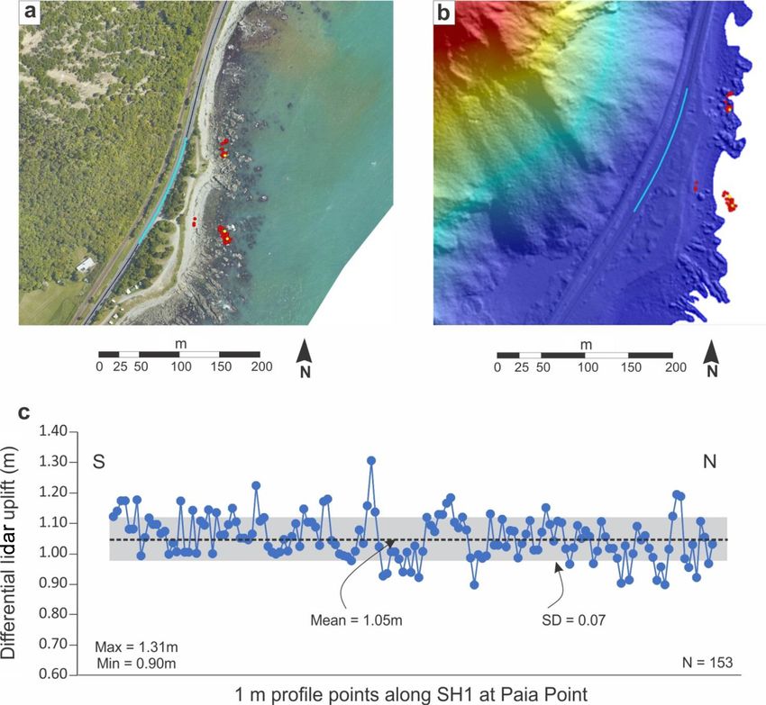
C. Reid et al.: Using a calibrated upper living position of marine biota to calculate coseismic uplift 353
of Kaikōura (Litchfield et al., 2018; Mouslopoulou et al.,
2019). The coastal section examined in this paper is crossed
by the Hundalee Fault (Fig. 1; see also Fig. 1c in Mous-
lopoulou et al., 2019), which accommodated a component
of reverse displacement and uplift of the coast up to ∼ 2 m.
In addition to the mapped surface faults, the spatial extent of
coastal uplift, the widespread occurrence of tsunamis (which
propagated for distances of up to ∼ 250 km from Kaikōura
south; Power et al., 2017) and the significant after-slip on
the plate interface suggest that faulting at the ground surface
was accompanied by slip on the subduction interface and an
offshore thrust fault that splays from the plate interface to ex-
tend within the accretionary prism complex (e.g. Cesca et al.,
2017; Mouslopoulou et al., 2019).
2.2 Physical and biological setting
The northern Canterbury coastline is predominantly ex-
posed to wave action, strikes northeast–southwest and is
broken only by the promontory of the Kaikōura Peninsula
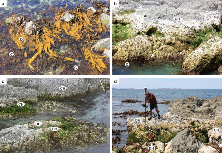
Figure 1. (a) Inset map of New Zealand illustrating the main (Fig. 1). Hinterland topography is steep and the coastal
tectonic features of the Hikurangi subduction margin, the loca- strip is narrow, comprising mainly greywacke bedrock be-
tion of the Marlborough Fault System (MFS) and the epicentre of neath bouldery shorelines interrupted by bays with gravel-
the 2016 Mw = 7.8 Kaikōura earthquake. The blue box near the dominated beaches. Prevailing winds from the northeast
Kaikōura earthquake epicentre indicates the study area. (b) Map (summer months) and southwest (winter months) main-
showing the study localities from which Durvillaea and Carpophyl-
tain year-round exposure, and the coastline supports biota
lum holdfast measurements were recorded using RTK GNSS and
adapted to this high-energy setting. The region is in a cool
tape measure, the position of State Highway 1 (SH1) from which
lidar data points were derived (see yellow line), the location of the temperate oceanographic setting with semi-diurnal tides with
Kaikōura tide gauge, and the KIKS strong-ground-motion station. a daily tidal variation of ∼ 2 m. These factors influence the
The Hundalee Fault is also located. The background image is sup- living positions of intertidal biota.
plied by Land Information New Zealand. The intertidal biota in this cool temperate setting is
dominated by seaweeds, typically the large brown algae
Durvillaea antarctica (bull kelp), D. willana, Carpophyllum
of at least 21 strike-slip, thrust and oblique-slip upper-plate maschalocarpum (Fig. 2a), and Hormosira banksii, coralline
faults that ruptured the ground surface and straddle the coast- algae (Fig. 2b), barnacles, limpets, chitons and mobile in-
line of the northeast South Island (Hamling et al., 2017; vertebrates (Marsden, 1985). Attached invertebrates, such as
Litchfield et al., 2018). The event’s complexity is reflected mussels and oysters, are present but not common on this
in the moment tensor of the main shock, which features stretch of coast. On the Kaikōura Peninsula species diver-
only 65 % to 75 % double-couple percentage (GEOFON; sity is high, with up to 78 species present in a single inter-
http://geofon.gfz-potsdam.de, last access: 20 March 2017) tidal transect (Marsden, 1985). The vertical distribution of
and is characterised by an oblique mechanism with compo- species on these rocky shores is controlled by exposure to
nents of thrusting and right-lateral slip. Fault ruptures gen- wave action and interspecies competition (Sharyn Goldstien,
erally propagated northwards from the epicentre for about personal communication, 2017). The rocky shores around
200 km, with a focal depth of the main shock at 15 km (Ham- Kaikōura support three major biozones that approximately
ling et al., 2017; Kaiser et al., 2017; Cesca et al., 2017). The correspond to tidal height: (a) an upper belt of littorinid gas-
resulting surface ruptures vary in strike from east–west to tropods (e.g. Littorina unifasciata and L. cincta) and barna-
north-northwest, with the faults having east-northeast strike cles (e.g. Epopella plicata); (b) a mid-tidal region dominated
being primarily right-lateral strike-slip and more northerly by grazing molluscs (e.g. Cellana denticulata, Melagraphia
striking faults accommodating strike-slip and reverse dis- aethiops and Turbo smaragdus); and (c) a lower zone of
placement (Nicol et al., 2018). The earthquake ruptured three brown algae (e.g. Durvillaea antarctica and Carpophyllum
faults (Hundalee, Papatea and Kekerengu faults) that cross maschalocarpum) (Marsden, 1985). When the shoreline was
the coastline and locally produced differential uplift of the inspected about 2.5 months after earthquake uplift, many mo-
rocky shorelines. Vertical displacement of −0.5 to +8 m oc- bile taxa were absent in the uplifted intertidal zone, and living
curred along > 100 km of coastline, with the highest values or dead remains of stranded encrusting or attached taxa, such
in the hanging wall of the reverse sinistral Papatea Fault north as barnacles, coralline algae and brown algae, dominated the
www.earth-surf-dynam.net/8/351/2020/ Earth Surf. Dynam., 8, 351–366, 2020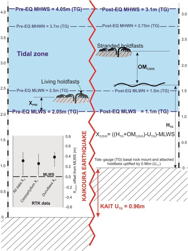
354                       C. Reid et al.: Using a calibrated upper living position of marine biota to calculate coseismic uplift

shoreline. The green alga Ulva is normally present in limited       indicators, tidal gauge measurements, remote sensing tech-
amounts (Marsden, 1985); however, following the Kaikōura           niques (RTK GNSS and lidar) and strong-motion recordings
earthquake and shoreline disturbance, growth of this alga           are used. The characteristics of each dataset collected and
was prolific and it subsequently covered much of the post-          the methodology used to derive tectonic uplift are presented
earthquake intertidal zone in the study area (Fig. 2b–d). This      below. All uplift data are available in the Supplement.
proliferation was accompanied by the death and bleaching of
stranded coralline red algae, forming a distinctive white crust     3.1   Kaikōura tide gauge
on rocky surfaces (Fig. 2b and d) which was often visible at
kilometre-scale distances; at that time, this was the most ob-      New Zealand has 15 tide gauges which record tidal vari-
vious visual indicator of uplift along the coastline.               ation, tsunami events, eustatic sea level changes and ver-
   In this study the brown algae Durvillaea and Carpophyl-          tical displacements of the coast. The Kaikōura tide gauge
lum are utilised to measure coastal uplift. Durvillaea is re-       (Fig. 1) measures sea level relative to two Druck PTX1830
stricted to the Southern Hemisphere and occurs on rocky             sensors (KAIT 40 and 41, each referenced to different da-
coastlines throughout New Zealand, while Carpophyllum is            tums) located at the end of the wharf at Kaikōura (WGS
endemic (Adams, 1994). Around the Kaikōura Peninsula and           84: −42.41288, 173.70277◦ ; NZTM: 1657824, 5304141).
north Canterbury coast, holdfasts of Durvillaea antarctica          In this study, data from the KAIT 41 sensor (http://apps.
(bull kelp) and D. willana (Fig. 2a) are anchored by a fleshy       linz.govt.nz/ftp/sea_level_data/KAIT/, last access: 5 Febru-
non-calcified holdfast to coralline encrusted rocky surfaces        ary 2017) are used exclusively to maintain internal consis-
in the lower intertidal zone (Adams, 1994; Nelson, 2013),           tency, although results would be the same had KAIT 40 been
and holdfasts extend subtidally by 1–2 m. Individual plants         used. The instrument is fixed to bedrock beneath the wharf;
have fronds 3–5 m in length that typically drape down from          it is referenced to nearby benchmarks, including one on the
the intertidal zone to depths of ∼ 5 m (Adams, 1994; Nel-           wharf itself (LINZ geodetic code EEFL), and records sea
son, 2013). On sites exposed to higher wave action, holdfasts       level at 1 min intervals. The data are recorded in UTC and the
of Durvillaea may appear higher in the intertidal zone due          water levels represent water surface elevation above the base
to increased wave wash (Marsden, 1985); however, in shel-           of the tide gauge in metres. The tide gauge was established
tered areas and sites where waves are baffled holdfasts may         in late May 2010 and operated continuously through the pe-
be subaerially exposed at spring low tides but not at neap low      riod of the 14 November Kaikōura earthquake, recording tec-
tides (Sharyn Goldstien, personal communication, 2017). By          tonic uplift at the site. KAIT 41 tide-gauge data assembled
contrast, Carpophyllum is only present in the low intertidal        for this study spanned the period from 1 December 2015 to
zone where it forms a distinct band close to low water (Nel-        7 February 2017 and indicate that tidal range varies between
son, 2013) (label C in Fig. 2c) and is not normally emergent        a spring tide average of ca. 2 and ca. 1.25 m during neap tides
at low spring tides (Sharyn Goldstien, personal communi-            (Table 1). Spring low tides before the Kaikōura earthquake
cation, 2017). Although both Carpophyllum and Durvillaea            registered ca. 2.05 m on the gauge, while spring high tides
may be present on open coasts (Fig. 2a), Durvillaea domi-           were ca. 4.05 m. After the earthquake, low-water spring tide
nates in exposed sites, and Carpophyllum is more abundant at        measured ca. 1.1 m and high-water spring ca. 3.1 m. Neap
relatively sheltered locations. Dead stranded and living rep-       tides measured ca. 2.5 m (low) and ca. 3.7 m (high) before
resentatives of one or both of these brown algae were present       the earthquake and ca. 1.5 m (low) and ca. 2.75 m (high) af-
at all the rocky coastal sites visited in this study, making Car-   ter the earthquake (Table 1).
pophyllum and Durvillaea an excellent combination of bio-               To determine the absolute uplift value from the tide-gauge
zone markers for measuring coseismic uplift.                        data (UTG ; see File S1 in the Supplement) we used the fol-
   The reproductive season for Durvillaea is during the             lowing methodology: (A) subtracted the high spring and high
winter months, peaking in August, and harvesting studies            neap tide readings before the earthquake from those after
have shown slow resettlement when fronds are removed in             the earthquake; (B) averaged high-tide and low-tide read-
September through February (Hay and South, 1979). The in-           ings from several tidal cycles (3 d period) before and after
tertidal zone on the Kaikōura coast is undergoing recovery         the earthquake; (C) aligned pre-earthquake tidal data with
from the November 2016 earthquake, and stabilised inter-            post-earthquake data and incrementally adjusted them until
tidal zones are not yet re-established. In temperate climate        achieving a best fit; (D) compared the average water eleva-
settings this may take several years, as shown by Castilla and      tion from a pre-earthquake month to the same month’s data
Oliva (1990) following the 1985 Chile earthquake.                   after the earthquake (e.g. December 2015 against Decem-
                                                                    ber 2016); and (E) calculated the difference in average wa-
                                                                    terline elevations for an extended period (44 d) before and
3   Methods                                                         after the earthquake (30 October to 27 December). The av-
                                                                    erage uplift (UTG ) estimated from the above steps (Tables 1
To measure coseismic uplift due to the Kaikōura earthquake,        and 2) is subsequently used to independently estimate the
independent methods utilising marine biological sea level           pre-earthquake upper range of the species used in this study

Earth Surf. Dynam., 8, 351–366, 2020                                                    www.earth-surf-dynam.net/8/351/2020/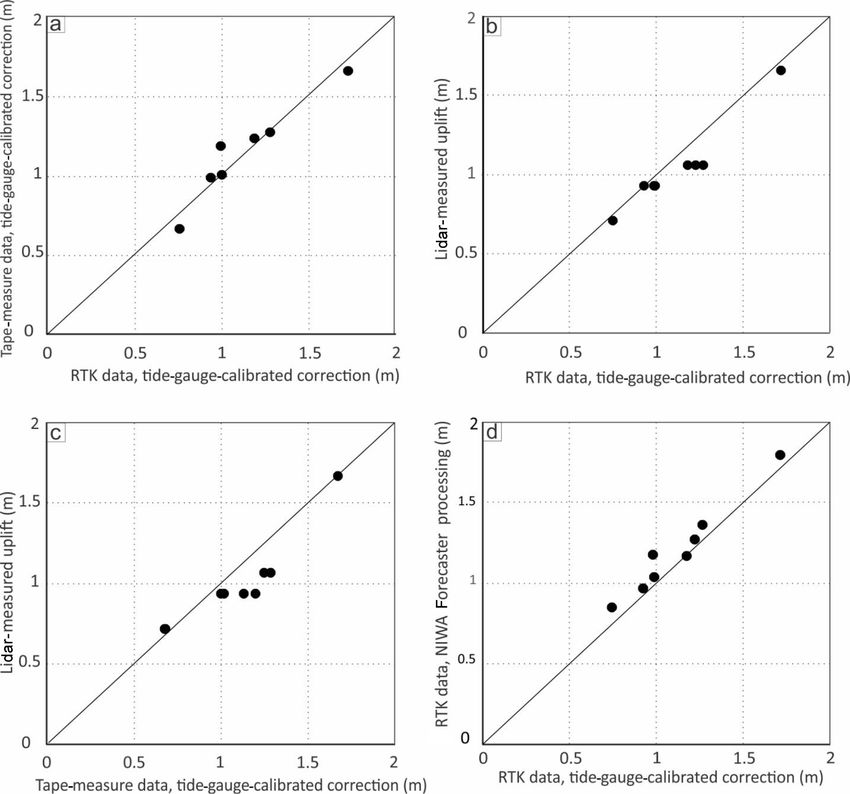
C. Reid et al.: Using a calibrated upper living position of marine biota to calculate coseismic uplift                                   355

Figure 2. Field photographs of the intertidal zone and biota near Kaikōura (taken after the earthquake). (a) Healthy Durvillaea (mostly
D. willana) (D) and Carpophyllum (C) photographed at low tide. (b) Uplifted bedrock north of Paia Point showing living Carpophyllum (C)
and dead Carpophyllum holdfast stumps (CH). Also note the living pink coralline algae at the waterline and bleached morbid coralline
algae (arrows) and bright green Ulva. (c) Uplifted intertidal zone near the Kaikōura tide gauge, showing a distinctive line of Carpophyllum
holdfasts (CH) and dispersed Durvillaea holdfasts (DH). (d) Uplifted intertidal zone near Paia Point. One of the authors (John Begg) is
measuring the elevation of Durvillaea holdfasts (DH) and Carpophyllum holdfasts (CH) using RTK GNSS survey equipment. Note the
distinctive white zone of dead coralline algae.

Table 1. Calculation of uplift at the Kaikōura tide gauge (KAIT) using tide-gauge readings for high and low spring tides as well as high and
low neap tides (see Sect. 3.1). Mean uplift is indicated in bold, derived by averaging the neap and spring low- and high-tide offsets.

                                          Spring tide                 Neap tide                      Uplift
                                      Pre-EQ     Post-EQ         Pre-EQ     Post-EQ        Spring diff.   Neap diff.
                         High tide     4.05 m       3.1 m         3.7 m       2.75 m       0.95 m             0.95 m
                         Low tide      2.05 m       1.1 m         2.5 m        1.5 m       0.95 m                1m
                         Range            2m          2m          1.2 m       1.25 m       Mean diff.         0.96 m

(see Sect. 3.2). It has also acted as a reference point against           the tide-gauge record for at least 12 h after the earthquake.
which all other instrumental and handheld measurements are                Further, a day after the earthquake, Kaikōura was subjected
compared.                                                                 to a southerly storm with powerful swells, and these are also
   Some limitations on calculating vertical displacement                  apparent in the tide-gauge data. These factors result in some
from tide-gauge records arise from the specific circum-                   blurring in the precision of uplift deriving from the difference
stances associated with the record around the 14 Novem-                   between pre-earthquake and post-earthquake data.
ber 2016 Mw = 7.8 Kaikōura earthquake. This event struck                    Uplift values calculated from tide-gauge data were com-
during a period of sharply increasing tidal change due to                 pared with those derived from lidar differencing data (see
high spring tides (related to lunar perigee and approaching               Sect. 3.4.1). Biological data from this site (see Sect. 3.2) were
solar perihelion) that culminated a few days after the earth-             used to calibrate the elevation of the upper extent of brown
quake. In addition, the earthquake generated a significant                algal holdfasts relative to sea level (in this case, MLWS).
tsunami (Power et al., 2017), the effects of which persist in

www.earth-surf-dynam.net/8/351/2020/                                                             Earth Surf. Dynam., 8, 351–366, 2020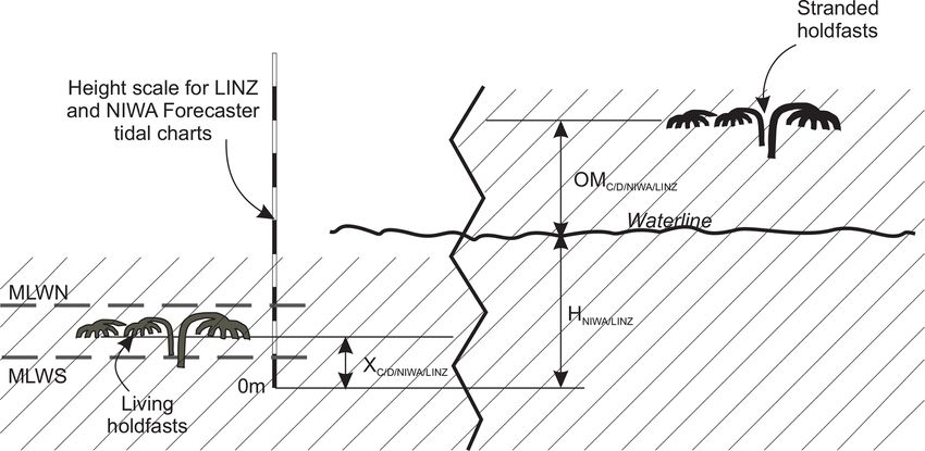
356                         C. Reid et al.: Using a calibrated upper living position of marine biota to calculate coseismic uplift

Table 2. Absolute uplift values calculated from the Kaikōura tide-      per holdfasts were measured (as they represent specimens
gauge data using methods B–E. Method B: comparison of average            closest to the pre-earthquake upper limit for each species).
high-tide and low-tide readings from several tidal cycles (3 d period)   In sites with boulders rather than bedrock exposure, only
before and after the earthquake. Method C: aligning pre-earthquake       boulders showing that a portion of their surface was clearly
tidal data with post-earthquake data and incrementally adjusting         within the pre-earthquake middle or upper tidal zone (evi-
them until a best fit. Method D: comparing the average water eleva-
                                                                         denced by bare or barnacle-encrusted surfaces) and that had
tion from a pre-earthquake month to the same month’s data after the
earthquake (December 2015 against December 2016). Method E:
                                                                         clearly remained undisturbed by strong ground shaking and
calculating the difference in average waterline elevations for an ex-    subsequent storm wave exposure were selected for measure-
tended period (44 d) before and after the earthquake (14 November        ment, therefore ensuring that the upper limit of holdfasts was
to 27 December). For Method A, we refer to the methodology estab-        represented.
lished in Sect. 3.1 and presented in Table 1. The overall mean uplift,      Two different methods were used to measure the vertically
UTG and standard deviation are shown in bold and are calculated          displaced biota. The primary method of collection of field
by summing mean uplift values from each method and dividing by           data was by a real-time kinematic global navigation satel-
the number of methods.                                                   lite system (RTK GNSS). At each site the water level was
                                                                         measured in the most sheltered area available to minimise
                Method      Data points        Mean                      wave effects, and the time the measurement was collected
                                               uplift
                                                                         was recorded. Following measurement of the waterline, up
                                                (m)
                                                                         to 20 holdfasts (either or both Carpophyllum and Durvil-
                A                              0.96                      laea) were measured within close proximity. Where addi-
                B           6                  0.95                      tional holdfasts were available at each site, the water level
                C           17 568             0.98                      was remeasured and further sets of up to 20 holdfasts mea-
                D           44 640             0.96                      sured. This RTK collection method did not require the wa-
                E           17 932             0.97
                                                                         terline measurement site and the holdfasts to be immediately
                Overall mean upliftUTG         0.96                      adjacent to each other. Additional biological data were col-
                  Standard deviation           0.02                      lected using a second method: direct tape measurement of
                                                                         the height of holdfasts above the water level. Tape measure-
                                                                         ments were collected between the waterline (measured be-
3.2   Biological data collection                                         tween wavelet peaks and troughs) and the upper algal hold-
                                                                         fasts on rock surfaces. Sheltered faces were again preferen-
Biological data collected comprised the location and eleva-              tially measured, although the requirement to have stranded
tion of approximately 400 stranded algal holdfasts during                holdfasts immediately adjacent to a measurable waterline
a 10 d period approximately 2.5 months after the Kaikōura               meant that sites exposed to wave wash were more commonly
earthquake (File S2). The decay of attached and uplifted                 used to achieve approximately 20 measurements. Each read-
biota was well advanced, and, in most cases, the uplifted                ing for both methods (RTK or tape) was annotated with the
remnants of marine algae, our primary target species, were               alga species measured, relative site exposure (exposed or
restricted to holdfast stumps of Durvillaea or Carpophyllum              sheltered) and the time of measurement.
with brittle fronds attached (Fig. 2b–d). Despite the decay of
algae, the position of the remaining stumps clearly reflected            3.3   Biological data processing
pre-earthquake algae distribution evidenced by a lack of rock
“scarring” whereby removed stumps might also remove other                These field measurements of holdfast heights were then pro-
intertidal biota and often expose fresh rock surfaces. The bi-           cessed to determine coseismic uplift, taking into account
ological data presented in this paper were collected close to            the time of data measurement within the tidal cycle and
the Kaikōura tide gauge on the northern side of the penin-              the pre-earthquake living position of algal holdfasts. Three
sula, Kaikōura Harbour on the south side and from two lo-               different methods were used for calculating tectonic uplift
calities along the south Kaikōura coastline: Paia Point and             from the vertical offsets of the biological horizons. These
Omihi Point (Fig. 1).                                                    were (a) tide-gauge calibration, (b) NIWA Tide Forecaster
   At all localities uplift was apparent from the exposure and           measurement and (c) LINZ tide prediction charts. The first
subsequent degradation of intertidal biota, with algal hold-             method utilised data from the Kaikōura tide gauge and differs
fasts exposed above the waterline, and measurements were                 significantly from the two tide prediction methods by cali-
collected on rising or falling mid-tides and low tides. Hold-            bration to real-time water-level records of the Kaikōura tide
fasts were preferentially measured on rock faces sheltered               gauge. The NIWA Forecaster and LINZ tidal chart methods
from, but retaining a connection to, the open sea to minimise            are included, however, to simulate locations where real-time
error introduction by the potentially higher tidal position of           tide gauges are not available. All data and calculations are
Durvillaea in wave-washed sites. Each site was visually as-              presented in File S2.
sessed to establish the upper extent of holdfasts, and the up-

Earth Surf. Dynam., 8, 351–366, 2020                                                        www.earth-surf-dynam.net/8/351/2020/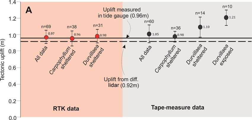
C. Reid et al.: Using a calibrated upper living position of marine biota to calculate coseismic uplift                                  357

Figure 3. Schematic diagram illustrating uplift and stranding of holdfasts at the Kaikōura tide gauge. It also schematically illustrates the
method for calculating uplift from the upper limit of holdfasts (XC/D/G ; Eq. 1) using mean low-water spring (MLWS) values within the tide-
gauge data. MLWN: mean low-water neap, MHWN: mean high-water neap, MHWS: mean high-water spring, HTG : tide height as measured
at the tide gauge, UTG : uplift as measured by tide-gauge offset data pre- and post-deformation, OM: observed measurement (holdfast), X:
offset of holdfasts from MLWS. Inset: results for X as calculated for kelp at the Kaikōura tide gauge. Mean values are shown by a solid
circle, while tails represent maxima and minima values. See Sect. 3.2.1 for details.

3.3.1   Deriving an upper living-position correction using               pre-earthquake datum, in this case the base of the tidal cycle
        the Kaikōura tide gauge (XC/D/G )                               mean low-water spring (MLWS). The Kaikōura tide gauge
                                                                         provides a record of the pre- and post-earthquake MLWS.
This new method determines an upper living position for                  First the height of the stranded holdfast is determined by
each species using the measured elevations of the stranded               adding the waterline height measured in the tide gauge (H )
holdfasts and then relating them to the pre-earthquake tidal             and the observed height of the holdfast above the waterline
cycle (Fig. 3) by subtracting uplift recorded by the tide                in sheltered locations (OM). The offset of MLWS pre- and
gauge. This enables the elevation of the holdfasts, which are            post-earthquake in the tide gauge calculated as uplift is sub-
being used to determine surface uplift, to be referenced to a

www.earth-surf-dynam.net/8/351/2020/                                                            Earth Surf. Dynam., 8, 351–366, 2020
358 C. Reid et al.: Using a calibrated upper living position of marine biota to calculate coseismic uplift
tracted, along with the height of MLWS in the tide gauge. online-services/tide-forecaster, last access: 5 March 2017)
This leaves a residual height that reflects the pre-earthquake that provide tidal predictions for sites between formal chart
elevation of holdfasts of each species with respect to MLWS. stations and attempt to account for local variation. For this
The upper holdfast living position is described here by calculation, Eq. (3) is used:
the correction XC/D , which is treated as a constant for
UB(NIWA) = HNIWA + OMC/D/G − XC/D_NIWA , (3)
Carpophyllum (XC ), Durvillaea (XD ) or a combination of
both (XG ). XC/D/G was determined by Eq. (1): where OMC/D/G is the observed elevation of the holdfasts
relative to locally measured sea level, HNIWA is the pre-
XC/D/G = HTG + OMC/D/G − UTG − MLWS, (1) dicted tide height from NIWA charts at the survey time,
and XC/D_NIWA is a correction value (NIWA-Forecaster-
where HTG is the waterline height at the tide gauge at the
calibrated correction) estimated to reflect the relative height
time of data collection (which can be accessed from http:
of Carpophyllum and Durvillaea within the tidal cycle
//www.linz.govt.nz/ (last access: 17 August 2017) and which
(Fig. 4). This value for X is independent of tidal gauge data
was averaged here over 10 min intervals to mitigate local
as used above and relies on the assessment of qualitative bi-
fluctuations). OMC/D/G is the observed height above the wa-
ological data only. As described in Sect. 2.2, Carpophyllum
terline for each stranded holdfast (determined by subtract-
in sheltered areas with a connection to the sea will not usu-
ing the RTK waterline height measurement from each RTK
ally be exposed at low spring tide (LST) (Sharyn Goldstien,
holdfast measurement per site or directly using tape mea-
personal communication, 2017). Tidal prediction charts over
surements; the subscripts C, D and G correspond to mea-
1 year were qualitatively assessed, and a mean low spring
surements for the different holdfasts). MLWS is the average
tide height of 0.1 m (XC_NIWA ) was estimated for the upper
tide-gauge reading for mean low-water spring tide (1.1 m for
limit of Carpophyllum and used as the correction value for
KAIT 41; see Table 1), and UTG is this uplift calculated at
this species in data processing. Likewise, Durvillaea will be
the tide gauge by the method described in Sect. 3.1.
regularly exposed at low spring tides but usually not exposed
As Carpophyllum and Durvillaea occupy slightly different
at low neap tide (Sharyn Goldstien, personal communication,
upper living positions in the intertidal zone, XC/D was calcu-
2017). A correction (XD_NIWA ) of 0.25 m was estimated, rep-
lated separately for each species. A general correction, XG ,
resenting a height between spring and neap low tides, rel-
using both Carpophyllum and Durvillaea holdfasts was also
evant to the Kaikōura region. These values for XC/D_NIWA
determined, to be applied at sites where holdfast species were
assume that the upper holdfast elevations of Carpophyllum
not known or determined or where insufficient numbers of
and Durvillaea are consistent between sheltered and exposed
each were available and data were pooled by necessity. To
areas.
calculate the correction, data were pooled by species irre-
The value of HNIWA was determined using the predicted
spective of site. The method described here uses the upper
tide heights and times from the NIWA Tide Forecaster web-
extent of intertidal algae as marker horizons, as at Kaikōura
site. The NIWA Tide Forecaster provides tide height at user-
these are readily available attached biota. However, biozone
designated locations that may be between the fixed LINZ lo-
boundaries for any attached intertidal organism with a re-
cations in order to accommodate the passage of tidal highs
stricted tidal range could be used to calculate this correction
and lows between fixed points. HNIWA was calculated using
factor.
the following equation (Eq. 4) from http://www.linz.govt.nz/
(last access: 5 March 2017):
3.3.2 Deriving tectonic uplift using the Kaikōura
tide-gauge method (UB(TG) ) HNIWA = h1 + (h2 − h1 ) [(cos A + 1)/2], (4)
Once the XC/D/G correction was derived as described above, where A = π ([(t −t1 )/(t2 −t1 )]+1) radians, t1 and h1 denote
coseismic uplift was calculated from biological data pooled the time and height of the tide (high or low) immediately pre-
by site in the location studied using Eq. (2): ceding time t, and t2 and h2 denote the time and height of the
tide (high or low) immediately following time t. Only time t
UB(TG) = HTG + OMC/D/G − MLWS − XC/D/G , (2) is measured; t1 , t2 , h1 and h2 are derived from predictive tide
charts.
where UB(TG) is the uplift calculated from biological data at
the Kaikōura tide gauge. 3.3.4 Process to derive tectonic uplift using the LINZ
tide prediction charts (UB(LINZ) )
3.3.3 Deriving tectonic uplift using the NIWA Tide
Land Information New Zealand (LINZ) tide charts available
Forecaster (UB(NIWA) )
at http://www.linz.govt.nz/ (last access: 5 March 2017) pro-
In order to calculate uplift from sites distant from the vide fixed tide prediction charts for New Zealand primary
tide gauge, RTK biological data were used in con- and secondary ports and were also used to derive HLINZ us-
junction with tidal charts (https://www.niwa.co.nz/services/ ing Eq. (3) as well as LINZ calibration correction values of
Earth Surf. Dynam., 8, 351–366, 2020 www.earth-surf-dynam.net/8/351/2020/C. Reid et al.: Using a calibrated upper living position of marine biota to calculate coseismic uplift 359
Figure 4. Schematic diagram illustrating the uplift and stranding of holdfasts used to calculate the offset of holdfasts (XNIWA/LINZ ) from
mean low-water spring (MLWS) independent from tide-gauge data. MLWN: mean low-water neap. Here MLWS is determined from LINZ
and NIWA predictive charts, and the position of holdfasts with respect to MLWS and MLWN is determined from local knowledge of kelp
distribution (Sharyn Goldstien, personal communication, 2017).
0.2 m for XC_LINZ and 0.4 m for XD_LINZ estimated as above 3.4 Differential lidar and strong-motion uplift estimates
from these charts. HLINZ was again determined by Eq. (4)
defined above, and only RTK data were processed this way. 3.4.1 Differential lidar (Ulidar )
Differential lidar has been developed along the
3.3.5 Sources of error coastal south Kaikōura region using pre-earthquake
(DEM_Kaikōura_2012_1m) and post-earthquake
Data points collected by RTK GNSS were accurate to ±5 cm,
(NZVD2016 and DEM_NZTA_1m) surveys of road
and this applies to both the waterline measurement at each
and railway routes using a common geodetic datum for each
site and each holdfast measurement. Both of these measure-
survey. To minimise the impact of gravity-induced slope
ments were used to derive OM, with a total error of ±10 cm.
failures and horizontal tectonic displacement on sloping
Manually collected biological data rely on the accuracy of
ground during the earthquake, the difference in the altitude
the waterline measurement taken. While sheltered microsites
of 1 × 1 pixels along the post-earthquake centreline of roads
were selected for these measurements, they were placed at an
was used. Specifically, for the Omihi Point and Paia Point
estimated median water level between wavelets. This error is
study localities (see Fig. 1) the nearby State Highway 1 was
more pronounced when measuring waterline heights at more
used, while for the Kaikōura tide-gauge study site, a section
exposed sites. Additionally, the time at which the measure-
of the coastal road near the wharf that houses the gauge
ment was taken may have occurred when the water level was
was used. The road sections that acted as a reference level
at either a positive or negative fluctuation from tidal predic-
have low relief (e.g. < 10 cm relief) and are wider than the
tion charts or tide-gauge readings for sites south of Kaikōura.
horizontal displacements recorded during the earthquake;
The total error is difficult to quantify; however, an assess-
thus, neither lateral tectonic displacement nor gravitational
ment of the Kaikōura tide-gauge data shows water-level fluc-
processes should significantly impact the differential lidar
tuations of less than ±0.1 m. Averaging tide-gauge data over
measurements. Collectively, a total of 510 differential lidar
10 min helped mitigate the error resulting from the tide gauge
points were collected and analysed (148 at the Kaikōura tide
itself; however, the error introduced by sea level fluctuations
gauge, 152 points at Paia Point and 210 points at Omihi
away from the tide gauge remained.
Point) (File S3). These data were used to produce mean
Durvillaea lives along open coasts, but at very exposed
uplift estimates of at each site with 2σ uncertainties of
sites pre-earthquake holdfasts would have sat higher than av-
±0.06–0.18 m (Table 6). Differential lidar data were not
erage in response to increased wave wash and run-up. This
available immediately adjacent to Kaikōura Harbour on the
potential error is difficult to quantify as deviation from aver-
south side of the peninsula.
age heights will be linked to wave heights and run-up at in-
dividual sites that may be modified following uplift. For this
reason, the most exposed sites were avoided (where possible) 3.4.2 Strong motion (USM )
and data were collected from sheltered locations.
A further independent instrumental uplift measurement
was achieved by calculating the static vertical displace-
www.earth-surf-dynam.net/8/351/2020/ Earth Surf. Dynam., 8, 351–366, 2020360 C. Reid et al.: Using a calibrated upper living position of marine biota to calculate coseismic uplift
Table 3. Results for the calculation of the upper living- Table 4. Comparison of uplift results for data collected by RTK
position XC/D/G relative to MLWS for holdfasts at the Kaikōura and tape measure at the tide gauge, including a comparison of kelp
tide gauge. Note that only holdfasts of Carpophyllum and Durvil- types in both sheltered and exposed locations. Results are presented
laea in sheltered locations were used to calculate this elevation. by holdfast species and exposure ranking independently of the col-
lection site.
Mean SD Median Max Min
All holdfasts XG 0.31 m 0.10 m 0.32 m 0.50 m 0.01 m Mean SD Min Max
Carpophyllum XC 0.26 m 0.09 m 0.26 m 0.43 m 0.01 m (m) (m) (m) (m)
Durvillaea XD 0.38 m 0.07 m 0.39 m 0.50 m 0.19 m
RTK data
All data 0.97 0.08 0.71 1.13
Carpophyllum sheltered 0.96 0.09 0.71 1.13
ment recorded by the nearby strong-motion site KIKS Durvillaea sheltered 0.98 0.07 0.78 1.09
(Fig. 1). The KIKS station is located 2.2 km south of the
Kaikōura tide gauge (lat., long.: −42.426◦ N, 173.682◦ E; Tape-measure data
NZTM: 1656161, 5302714; see Fig. 1) and operated by All data 1.05 0.11 0.87 1.35
GeoNET. The Kinemetrics FBA-ES-T-BASALT 2420 sensor Carpophyllum sheltered 0.98 0.06 0.87 1.13
is located at 8 m of elevation on the concrete floor of a single- Carpophyllum exposed 1.06 0.07 0.92 1.22
storey building at Kaikōura Harbour. Ground acceleration is Durvillaea sheltered 1.10 0.13 0.91 1.35
recorded with a period of 0.005 s and data can be downloaded Durvillaea exposed 1.21 0.09 1.07 1.35
online from ftp://ftp.geonet.org.nz/strong/processed/ (last ac-
cess: 5 March 2017).
Static displacement was calculated from the vertical com- using an RTK GNSS and a tape measure produce uplift esti-
ponent of the instrument following the method of Wang et mates that are, within the uncertainties given, indistinguish-
al. (2011) and using their software package smbloc, which able from uplift recorded by the tide gauge (0.96 m) and dif-
applies an empirical baseline correction to remove linear pre- ferential lidar (0.92 cm) (Fig. 5). By contrast, estimates of
and post-event trends in the data. Static displacement derived uplift using Durvillaea are always higher than tide-gauge and
with this method after large earthquakes has been shown differential lidar values. Tape measurements of Durvillaea
to be robust (e.g. Schurr et al., 2012). Here, the resulting produced the highest biological uplift estimates with exposed
vertical displacement for the KIKS strong-motion station is Durvillaea recording a mean uplift of 1.21 m, which is 0.25–
0.87 ± 0.06 m (see Table 6 and File S4 for further details on 0.29 m above the tide-gauge and differential lidar values (Ta-
data processing). ble 4, Fig. 5). These data suggest that Durvillaea should be
regarded as providing maximum uplift estimates, supporting
previous work in suggesting that Durvillaea at exposed sites
4 Results and comparison of methods
should be used with caution (e.g. Clark et al., 2017).
4.1 Kaikōura tide-gauge locality The same biological data collected near the Kaikōura tide
gauge were then grouped by data collection location (sets
Tide-gauge data indicate that the Kaikōura tide gauge was of approximately 20 data points) rather than holdfast type,
coseismically uplifted by 0.96 ± 0.02 m (UTG ) (Tables 1 and uplift estimates produced results of 0.99 m ± 0.07 m,
and 2) (see Sect. 3.1) and represents a key reference point 0.92 m ± 0.10 m and 0.98 m ± 0.07 m, while tape mea-
for this study. In addition to providing an independent esti- sures resulted in uplift estimates of 1.00 m ± 0.07 m,
mate of uplift, the tide-gauge data have been used to calcu- 1.12 m ± 0.11 m and 1.19 m ± 0.08 m, respectively (Fig. 6a,
late the upper living-position correction factor XC/D/G from Table 5). In addition to directly measuring water levels at
all stranded biological holdfast data collected proximal to the the tide gauge, the NIWA Forecaster and LINZ tide charts
tide gauge (Eq. 1) (Table 3; Fig. 5). were used to calculate uplift in an effort to test the utility
The calculated corrections XC/D (Table 3) were applied to of tide charts at remote locations where tide-gauge and in-
biological measurements collected proximal to the Kaikōura strument data may not be available. These comparisons are
tide gauge (Fig. 5) and compared with uplift of the Kaikōura illustrated in Table 5 and Fig. 6. At the tide-gauge site, the
tide gauge (calculated in Sect. 3.1). RTK GNSS survey data LINZ tide chart produced, for Carpophyllum, uplift results
of Durvillaea and Carpophyllum for sheltered and exposed 0.11–0.12 m greater than the tide-gauge method, while an
holdfasts produce tectonic uplift values of 0.71 to 1.13 m, NIWA Forecaster chart produced uplift estimates of 0.04–
with a mean of 0.97 ± 0.08 m (Table 4, Fig. 5). Similarly, for 0.05 m greater than the tide-gauge mean (Table 5). As was
all tape-measure data collected proximal to the tide gauge, the case for the tide-gauge calibration method, Durvillaea
tectonic uplift estimates range between 0.87 and 1.35 m, with produced the greatest uplift at the tide gauge using the tide-
a mean of 1.05 ± 0.11 (Table 4, Fig. 5). The resulting anal- chart method, with average uplift values of 1.18 and 1.24 m.
ysis suggests that Carpophyllum at sheltered sites recorded In summary, uplift estimates calculated from Carpophyllum
Earth Surf. Dynam., 8, 351–366, 2020 www.earth-surf-dynam.net/8/351/2020/C. Reid et al.: Using a calibrated upper living position of marine biota to calculate coseismic uplift 361
Figure 5. Uplift at the Kaikōura tide gauge calculated from the upper living positions of various kelp holdfasts and exposure sites plotted
against the offset recorded at the same locality using the tide gauge and differential lidar. Holdfast data are presented as the mean and standard
deviation, while the tide-gauge and lidar data are presented as the mean only. Black numbers beside the data points indicate the mean values,
while n values at the top represent the number of measurements per category.
holdfasts processed using the NIWA Forecaster tide charts
(rather than LINZ charts) are the most similar to direct uplift
of the tide gauge itself, to the tide-gauge biological results
Table 5. Comparison of mean uplift values derived using RTK and to lidar (plus 0–0.25 m), promoting their use in circum-
for the various methodologies (e.g. tide-gauge calibration method, stances in which a tide gauge is unavailable. LINZ tide-chart
NIWA Forecaster method, LINZ tide-chart method). As the source methods produced results within 0.32 m of other methods.
data remain identical for each method, the standard deviation re-
flects error derived from the RTK measurements. Data are presented
by site at each location; when a site was sampled using both Car- 4.2 Kaikōura harbour, Paia Point and Omihi Point
pophyllum and Durvillaea, the holdfast type is recorded as “mixed”.
To further test the utility of the Kaikōura calibration method
Site Holdfast type Tide- NIWA LINZ SD∗
and the other methods under consideration, algae uplift data
gauge Forecaster tide- (m) were also processed from the Kaikōura Harbour, Paia Point
mean mean chart and Omihi Point sites. Data from these locations are not as
(m) (m) mean detailed as those collected at the tide-gauge study site itself,
(m)
with the distinction between Carpophyllum and Durvillaea
RTK as well as sheltered and exposed areas not always available.
Tide gauge 1 Carpophyllum 0.99 1.04 1.11 0.06 At Paia Point, uplift estimates from all data collection and
Tide gauge 2 Carpophyllum 0.92 0.97 1.04 0.10 processing methods range from 1.12 to 1.36 m, with a mean
Tide gauge 3 Durvillaea 0.98 1.18 1.24 0.07 uplift of 1.24 m ± 0.16 m (Table 5; Fig. 6). While the biolog-
Paia Point 1 Carpophyllum 1.27 1.27 1.24 0.11
Paia Point 2 Durvillaea 1.22 1.36 1.36 0.18 ical uplift results are internally consistent, on average they
Paia Point 3 Mixed 1.18 1.17 1.12 0.16 are about 0.2 m higher than the differential lidar average up-
Omihi Point 1 Carpophyllum 1.71 1.80 1.95 0.13 lift at this site, which is 1.05 m ± 0.07 m (Table 6; Fig. 7).
Kaikōura Hbr Carpophyllum 0.74 0.85 0.98 0.12 This higher estimate for biological data cannot be attributed
Tape measure to differences in species of algae or measurement technique;
Tide gauge 1 Carpophyllum 1.00 0.07 however, shoreline exposure to wave action cannot be ex-
Tide gauge 2 Carpophyllum 1.12 0.11 cluded as a factor. The role of shoreline exposure may only
Tide gauge 3 Durvillaea 1.19 0.08 be resolved once the uplifted shoreline is recolonised with
Tide gauge 4 Mixed 0.99 0.06
new Carpophyllum and Durvillaea. Algal uplift measure-
Paia Point 1 Mixed 1.27 0.09
Paia Point 2 Mixed 1.23 0.09 ments collected at Omihi Point (Fig. 1) and processed using
Omihi Point 1 Mixed 1.66 0.17 the tide-gauge calibration correction XC/D are within 0.07 m
Kaikōura Hbr Carpophyllum 0.66 0.10 of one another and uplift recorded by differential lidar (Ta-
Kaikōura Hbr Carpophyllum 0.67 0.06 bles 5 and 6, Fig. 6). RTK measurements from Omihi Point
processed using the NIWA Forecaster and LINZ tide-chart
methods are 0.08 and 0.23 m, respectively, above tide-gauge-
calibrated estimates. In summary, there is no systematic dif-
www.earth-surf-dynam.net/8/351/2020/ Earth Surf. Dynam., 8, 351–366, 2020362 C. Reid et al.: Using a calibrated upper living position of marine biota to calculate coseismic uplift
Table 6. Uplift calculated from differential lidar and strong-motion
uplift estimated from the KIKS station.
Mean Median SD Max Min
(m) (m) (m) (m) (m)
Differential lidar
Tide gauge 0.92 0.91 0.06 1.13 0.77
Paia Point 1.05 1.05 0.07 1.31 0.90
Omihi Point 1.64 1.64 0.04 1.74 1.53
KIKS strong motion
Kaikōura Harbour 0.87 0.06
results from other methods, although all biological methods
produce uplift estimates that are higher than lidar results. The
tide-gauge-calibrated method has yielded results most con-
sistent with lidar. At all sites uplift estimated using the tide-
gauge calibration method give results within 0.0 to +0.21 m
(or 0.35 % to 21 %) higher than lidar results, with a mean of
+0.11 m (10 %). Further, at all sites and over all biological
methods, uplifts estimates are 0.0 to +0.31 m (or < 34 %)
higher than associated lidar results, with a mean of +0.17 m.
5 Discussion
The distribution of kelp within the intertidal zone at Kaikōura
Figure 6. (a) Tectonic uplift in metres measured at the Kaikōura
is well defined with respect to qualitative upper, middle and
tide gauge, Kaikōura Harbour, Paia Point and Omihi Point from
lower intertidal zones (Marsden, 1985). Nevertheless, be-
biological data processed using the tide-gauge correction, as well
as NIWA and LINZ predictive tide-chart correction methods (see cause the width of the intertidal zone varies with site expo-
Sect. 3.2). These values are compared to uplift recorded by the tide sure, topography, wave wash and competition between differ-
gauge and differential lidar (where available). (b) Percentage of up- ent organisms, an attempt to quantify this uncertainty is made
lift deviation of the biological methods with respect to the lidar mea- by calibrating coseismically uplifted intertidal brown algae
surements. Horizontal axis not to scale. (Durvillaea and Carpophyllum) in the immediate vicinity of
the Kaikōura tide gauge, aiming to establish a quantitative
correction value for the upper living position of the kelp hold-
ference in the uplift estimates at Paia Point and Omihi Point fasts with respect to MLWS (Figs. 3 and 5).
between the different measurement techniques (RTK GPS Using Eq. (1) (see Sect. 3.2) at the Kaikōura tide gauge, an
vs. tape measure), species of algae (Carpophyllum or Durvil- upper living-position correction of XC of 0.26±0.09 m above
laea) or tide charts (NIWA Forecaster or LINZ tide chart) MLWS is derived for sheltered Carpophyllum maschalo-
(Fig. 6). carpum. For Durvillaea in sheltered sites, the upper living-
At the Kaikōura Harbour site, where the KIKS seis- position correction XD is 0.38±0.09 m above MLWS. These
mic station is located (Fig. 1), uplift estimates from values were subsequently used to estimate tectonic uplift at
biological data, processed with the tide-gauge-calibrated sites located up to 15 km from the tide gauge and produced
upper living-position methodology, are 0.74 m ± 0.12 m uplift measurements which were in good agreement with
and 0.85 m ± 0.12 m for NIWA-calibrated methods and uplift calculated at the same localities by differential lidar
0.98 m ± 0.12 m for LINZ methods. These results bracket (Figs. 6 and 7). Thus, it appears that this method of estimat-
the uplift result recorded by the strong-motion data of ing correction values may be important as it provides, for the
0.87 m ± 0.06 m (Fig. 6). Differential lidar was not available first time, an independent quantitative method for estimating
adjacent to Kaikōura Harbour for comparison with biological the preferred upper living position for intertidal biota with
measurements respect to MLWS. This method may be applied elsewhere
Comparison of results for all biological methods, indepen- to other intertidal biota in the vicinity of a tide gauge. Car-
dent of location, shows a consistent correlation (Fig. 8). No pophyllum is endemic to New Zealand, while Durvillaea is
single method stands out as producing persistently divergent widespread in the Southern Hemisphere. The derived correc-
Earth Surf. Dynam., 8, 351–366, 2020 www.earth-surf-dynam.net/8/351/2020/C. Reid et al.: Using a calibrated upper living position of marine biota to calculate coseismic uplift 363 Figure 7. Locality, digital elevation imagery and differential lidar data for Paia Point (see Fig. 1 for location). (a) Aerial photo from Google Earth© imagery of Paia Point, State Highway 1 and uplift collection points. Blue line: portion of SH1 from which differential lidar uplift was calculated; red circles: RTK-GPS-collected kelp data points; yellow circles: tape-measure-collected kelp data points. (b) Digital elevation model developed from post-earthquake lidar data. Blue line and colour-coded circles as per (a). (c) Plot of uplift of points at 1 m intervals along the blue line on SH1 in (a) and (b) derived from differential lidar. tions are specific to these taxa in the Kaikōura region, which for biological data collected proximal to the tide gauge is is characterised by a moderate tidal range. If these values well mitigated by the use of the real-time tide-gauge water are applied elsewhere, the uncertainty would be equal to the level (H ), away from the Kaikōura tide gauge this real-time maximum correction value of 0.38 m. The three biological fluctuation is less able to be mitigated. Therefore, the NIWA post-processing methods used to obtain uplift all yield re- and LINZ tidal chart calculations for H , and the associated sults which are, within uncertainties, similar to one another, corrections, may give equally accurate uplift estimates. Over- meaning that any of these methods could be applied depend- all, the NIWA method produces results more consistent with ing on the available tidal data at the site of interest. Analysis non-biological methods than the LINZ method. Despite this, of all data suggests that handheld measurements most often data collected by RTK and processed using predictive charts, overestimate uplift compared to results from RTK GPS sur- such as LINZ, may be used to calculate uplift estimates and vey data. could be used with confidence in remote locations or loca- In the vicinity of the Kaikōura tide gauge, biological re- tions where other methods are not available. sults using the tide-gauge correction are most similar to non- This study has shown that instrumental and biological biological methods. With increasing distance from the tide methods can produce comparable results; yet, in order to re- gauge, this new method provides reliable results; neverthe- duce uncertainty in the biological methods, the biota should less, other biological methods were comparable. Progression have a living position relative to an appropriate sea level da- of daily tides is even, and fluctuations from the expected tum that is calibrated against real-time tide-gauge data. To tidal progression may occur over several minute intervals this end, our study has provided a new calibration method due to natural unevenness in the ocean surface caused by to derive a correction for this upper living position that can wind, barometric pressure and local topography (e.g. Gar- be applied globally where tide-gauge records are available. rison, 2010). While the influence of this natural fluctuation In circumstances in which tide-gauge records are unavail- www.earth-surf-dynam.net/8/351/2020/ Earth Surf. Dynam., 8, 351–366, 2020
You can also read