US EPA EnviroAtlas Meter-Scale Urban Land Cover (MULC): 1-m Pixel Land Cover Class Definitions and Guidance - remote ...
←
→
Page content transcription
If your browser does not render page correctly, please read the page content below
remote sensing
Article
US EPA EnviroAtlas Meter-Scale Urban Land Cover
(MULC): 1-m Pixel Land Cover Class Definitions
and Guidance
Andrew Pilant 1, *, Keith Endres 1 , Daniel Rosenbaum 2          and Gillian Gundersen 3
 1    MD243-05, Office of Research and Development, United States Environmental Protection Agency,
      Research Triangle Park, NC 27711, USA; endres.keith@epa.gov
 2    Oak Ridge Institute for Science and Education, P.O. Box 117, Oak Ridge, TN 37831, USA;
      rosenbaum.daniel@epa.gov
 3    Oak Ridge Associated Universities Inc., P.O. Box 117, Oak Ridge, TN 37831, USA; gillgundersen@gmail.com
 *    Correspondence: pilant.drew@epa.gov

 Received: 6 May 2020; Accepted: 9 June 2020; Published: 12 June 2020

 Abstract: This article defines the land cover classes used in Meter-Scale Urban Land Cover (MULC),
 a unique, high resolution (one meter2 per pixel) land cover dataset developed for 30 US communities
 for the United States Environmental Protection Agency (US EPA) EnviroAtlas. MULC data categorize
 the landscape into these land cover classes: impervious surface, tree, grass-herbaceous, shrub,
 soil-barren, water, wetland and agriculture. MULC data are used to calculate approximately 100
 EnviroAtlas metrics that serve as indicators of nature’s benefits (ecosystem goods and services).
 MULC, a dataset for which development is ongoing, is produced by multiple classification methods
 using aerial photo and LiDAR datasets. The mean overall fuzzy accuracy across the EnviroAtlas
 communities is 88% and mean Kappa coefficient is 0.84. MULC is available in EnviroAtlas via
 web browser, web map service (WMS) in the user’s geographic information system (GIS), and as
 downloadable data at EPA Environmental Data Gateway. Fact sheets and metadata for each MULC
 community are available through EnviroAtlas. Some MULC applications include mapping green
 and grey infrastructure, connecting land cover with socioeconomic/demographic variables, street
 tree planting, urban heat island analysis, mosquito habitat risk mapping and bikeway planning.
 This article provides practical guidance for using MULC effectively and developing similar high
 resolution (HR) land cover data.

 Keywords: high spatial resolution land cover data; remote sensing; EnviroAtlas; ecosystem services;
 decision support; image classification; machine learning; object-based image classification; rule-based
 image classification; pixel-based image classification; GIS; 1 m pixel

1. Introduction
     Land cover (LC) data indicate the type, extent and configuration of the physical materials present
at earth’s surface (e.g., vegetation, built surfaces) and are essential to informed, effective stewardship
of community landscapes, supporting decision making that integrates ecological, social, and economic
factors. Toward this integration, the United States Environmental Protection Agency (US EPA) created
EnviroAtlas (www.epa.gov/enviroatlas), a collection of interactive geospatial tools and resources that
allows users to explore the many benefits people receive from nature, often referred to as ecosystem
goods and services (EGS) [1]. Key components of EnviroAtlas are a multi-scaled interactive map, which
provides easy access to EnviroAtlas data, the Eco-Health Relationship Browser, which shows linkages
between ecosystems, the services they provide, and human health [2], and ecosystem services information
and educational resources, including a range of lesson plans that educators may integrate into classrooms.

Remote Sens. 2020, 12, 1909; doi:10.3390/rs12121909                        www.mdpi.com/journal/remotesensing
Remote Sens. 2020, 12, 1909 2 of 19
EnviroAtlas is organized at two spatial scales. A coarser national-scale component spans
Remote Sens. 2019, 11 FOR PEER REVIEW 2
the
conterminous US and builds on the US National Land Cover Dataset (NLCD) [3] with a 30 × 30 m pixel
resolution.
[2], andFor a finer community-scale
ecosystem services informationcomponent,
and educational the EnviroAtlas team has
resources, including developed
a range of lessonMeter-Scale
plans
Urban that educators
Land Covermay integrate
(MULC) at into
1 × classrooms.
1 m per pixel resolution, to support analysis and visualization
of ecosystemEnviroAtlas
servicesisatorganized at tworesolution
a fine spatial spatial scales.
thatAcaptures
coarser national-scale
individual trees, component
buildings spansandtheroads
(Figures 1 and 2). For comparison, there are nine hundred MULC 1 × 1 m pixels to one m
conterminous US and builds on the US National Land Cover Dataset (NLCD) [3] with a 30 × 30 NLCD
pixel resolution. For a finer community-scale component, the EnviroAtlas team has developed Meter-
30 × 30 m pixel. A webmap of MULC examples can be found here: https://arcg.is/0fXjue0. As of 2020,
Scale Urban Land Cover (MULC) at 1 × 1 m per pixel resolution, to support analysis and visualization
there are 30 published EnviroAtlas MULC datasets: Austin, TX; Baltimore, MD; Birmingham, AL;
of ecosystem services at a fine spatial resolution that captures individual trees, buildings and roads
Brownsville,
(Figures 1TX;andChicago, IL; Cleveland,
2). For comparison, OH;nine
there are Deshundred
Moines, IA; Durham,
MULC NC; to
1 × 1 m pixels Fresno,
one NLCD CA; 30 Green
× 30 Bay,
WI; Los Angeles County, CA; Memphis, TN; Milwaukee, WI; Minneapolis/St.
m pixel. A webmap of MULC examples can be found here: https://arcg.is/0fXjue0. As of 2020, there Paul, MN; New Bedford,
MA; are
New30Haven,
published CT; EnviroAtlas
New York, NY; MULC Patterson,
datasets:NJ; Philadelphia,
Austin, PA; Phoenix,
TX; Baltimore, AZ; Pittsburgh,
MD; Birmingham, AL; PA;
Portland, ME; Portland,
Brownsville, TX; Chicago,OR;IL;Salt Lake City,
Cleveland, OH;UT; Des Sonoma
Moines, IA;County,
Durham, CA;NC;St.Fresno,
Louis, CA;MO; Tampa,
Green Bay, FL;
WI; Beach,
Virginia Los Angeles County, CA;D.C.;
VA; Washington, Memphis,
Woodbine, TN; Milwaukee,
IA. WI; Minneapolis/St. Paul, MN; New
The term “meter-scale” indicates the general size range of NJ;
Bedford, MA; New Haven, CT; New York, NY; Patterson, Philadelphia,
the smallest PA; Phoenix,
identifiable features AZ;on the
Pittsburgh, PA; Portland, ME; Portland, OR; Salt Lake City, UT; Sonoma County,
ground. This corresponds to objects approximately one to four meters in size. The size of the smallest CA; St. Louis, MO;
Tampa, FL; Virginia Beach, VA; Washington, D.C.; Woodbine, IA.
detectable features varies, depending largely on the spectral and spatial contrast of the target against
The term “meter-scale” indicates the general size range of the smallest identifiable features on
its background. Image quality, date and atmospheric conditions are also factors.
the ground. This corresponds to objects approximately one to four meters in size. The size of the
Similar high spatial
smallest detectable resolution
features (HR) landlargely
varies, depending coveron(LC) data products
the spectral and spatial have beenofdeveloped
contrast the target by
otheragainst
groups, its translated
background.toImage MULC, anddate
quality, incorporated
and atmosphericinto EnviroAtlas.
conditions are These external sources are
also factors.
the University
Similarof Vermont
high Spatial Analysis
spatial resolution (HR) landLab, cover Sonoma
(LC) dataVeg Map,have
products the State of Iowa, by
been developed Chesapeake
other
Conservancy, Central Arizona-Phoenix (CAP LTER), Oneida Total Integrated Enterprises the
groups, translated to MULC, and incorporated into EnviroAtlas. These external sources are (OTIE),
University
University of VermontCenter
of Arkansas Spatialfor
Analysis
AdvancedLab, Sonoma
Spatial Veg Map, the State
Technologies, andofthe Iowa, Chesapeake
Missouri Resource
Conservancy,
Assessment Central Arizona-Phoenix
Partnership (MoRAP). After(CAP LTER),
external LCOneida
data Total Integrated to
are translated Enterprises
the MULC (OTIE),
system,
University of Arkansas Center for Advanced Spatial Technologies, and the Missouri Resource
such data are considered equivalent to MULC, and are accompanied by the full suite of EnviroAtlas
Assessment Partnership (MoRAP). After external LC data are translated to the MULC system, such
community EGS metrics. External land cover data sources, and how those data are translated to MULC,
data are considered equivalent to MULC, and are accompanied by the full suite of EnviroAtlas
are specified in metadata for each MULC community.
community EGS metrics. External land cover data sources, and how those data are translated to
As of 2010,
MULC, approximately
are specified 81 percent
in metadata for eachofMULCthe United States (US) population lived in “urban areas”
community.
(US Census As of 2010, approximately 81 percent of the United States >
terminology for communities with population 2500)
(US) [4]. Expanding
population urbanization
lived in “urban areas” is
one motivation for developing
(US Census terminology high spatialwith
for communities resolution
population urban LC[4].
> 2500) data for EnviroAtlas
Expanding urbanization Communities.
is one
motivationcommunity
By modelling for developing high spatial
landscapes resolution
at the fine MULC urbanspatial
LC datascale
for EnviroAtlas
of individual Communities. By
streets, buildings,
trees,modelling
and lawns, community landscapes
we are better able atto the fine MULC
quantify spatialproperties
landscape scale of individual streets,that
and patterns buildings,
contribute
trees, and
to human lawns, weand
well-being are healthy
better ableurban
to quantify landscape
ecosystems properties
(Figures and 2)
1 and patterns
and thesethat contribute
EGS may to then
human well-being and healthy urban ecosystems (Figure 1 and Figure 2) and these EGS may then be
be better represented in making community decisions and policy. Potential MULC users include
better represented in making community decisions and policy. Potential MULC users include
planning, commerce, transportation, recreation and public health authorities; water, wildlife and
planning, commerce, transportation, recreation and public health authorities; water, wildlife and
natural resource managers; community decision makers, teachers, students and citizens.
natural resource managers; community decision makers, teachers, students and citizens.
Figure 1. Comparison of spatial scale and level of detail of (a) Meter-Scale Urban Land Cover (MULC)
(1 m pixel) and (b) National Land Cover Dataset (NLCD) (30 m pixel) in a Pittsburgh, PA neighborhood
and golf course. Land cover 50% transparency over NAIP imagery.
Remote Sens. 2019, 11 FOR PEER REVIEW                                                                        3

            Figure 1. Comparison of spatial scale and level of detail of (a) Meter-Scale Urban Land Cover (MULC)
Remote Sens.(12020, 12, 1909and (b) National Land Cover Dataset (NLCD) (30 m pixel) in a Pittsburgh, PA
                m pixel)                                                                                            3 of 19
            neighborhood and golf course. Land cover 50% transparency over NAIP imagery.

           Figure
      Figure       2. MULC
              2. MULC       examples
                         examples for for
                                      sixsix of thirty
                                          of thirty    EnviroAtlascommunities.
                                                    EnviroAtlas    communities. The
                                                                                The six
                                                                                     six inset
                                                                                          insetmaps
                                                                                               mapsshow
                                                                                                     showMULC
                                                                                                           MULC for
           forthe
      each of   each  of the EnviroAtlas
                  EnviroAtlas             communities,
                               communities,               with an expanded
                                                with an expanded              inset MULC
                                                                     inset showing  showingat MULC
                                                                                                higher at higher
                                                                                                       magnification.
           magnification. Community boundaries are from 2010 Census Urban Areas plus 1 km buffer.
      Community boundaries are from 2010 Census Urban Areas plus 1 km buffer.

           The purpose of this paper is to define the EnviroAtlas MULC land cover classes, describe the
     The purpose of this paper is to define the EnviroAtlas MULC land cover classes, describe the
      processes used to generate MULC, and provide guidance to support the most effective use of MULC
processes used to generate MULC, and provide guidance to support the most effective use of MULC
      data. In the Materials and Methods section, we present the MULC design, aerial imagery and LiDAR
data. data
       In the  Materials and
           specifications,      Methods
                            image           section,
                                   classification    we present
                                                  methods         the MULC
                                                           and a fuzzy        design,
                                                                        accuracy       aerialmethod.
                                                                                 assessment   imageryNext,
                                                                                                       andwe LiDAR
data define
      specifications,
              the MULC classes and their characteristics. The Results section summarizes statistics for 30 USNext,
                         image   classification   methods    and  a fuzzy  accuracy   assessment    method.
we define    the MULC
      EnviroAtlas          classes The
                    communities.    andDiscussion
                                         their characteristics.   The Results
                                                     section highlights        section
                                                                        some MULC       summarizes
                                                                                     applications     statistics for
                                                                                                  and practical
30 USguidance
        EnviroAtlas     communities.
                 for interpreting MULCThe  data.Discussion section highlights some MULC applications and
practical guidance for interpreting MULC data.
      2. Materials and Methods
2. Materials
         Theand Methods
             MULC classes are intended to represent common urban landscape composition and features
     that MULC
     The  can be reliably
                   classesidentified in 1 ×to1represent
                           are intended        m pixels, visible
                                                         common  near-infrared digital aerial
                                                                    urban landscape           photography,
                                                                                        composition        by
                                                                                                      and features
     human aerial photo interpreters, and by computer image classification algorithms. MULC
that can be reliably identified in 1 × 1 m pixels, visible near-infrared digital aerial photography, by
     classification design considerations include:
human aerial photo interpreters, and by computer image classification algorithms. MULC classification
     •    encompass the LC types anticipated in US community landscapes;
design
     •
        considerations   include:
          these LC classes are broadly recognized and understood by users;
     •    simplicity;
•    encompass    the LC types anticipated in US community landscapes;
     •    the size of discrete landscape objects and features readily classifiable in single date, 1 × 1 m
•    thesepixel
           LC classes
                imagery;
                         are broadly recognized and understood by users;
•    simplicity;
     •    minimal confusion between classes;
•    the
     •    size of
          broad      discrete
                 range           landscape
                        of potential          objects and features readily classifiable in single date,
                                     applications.
     1 × 1The   Levelimagery;
           m pixel     1 MULC classes are: water, impervious surface, soil-barren, tree, shrub, grass,
•    agriculture  and wetlands.
      minimal confusion     between To classes;
                                       date, the more specific Level 2 classes have been used only as
•    broad range of potential applications.

     The Level 1 MULC classes are: water, impervious surface, soil-barren, tree, shrub, grass, agriculture
and wetlands. To date, the more specific Level 2 classes have been used only as intermediate classes
during the classification stage; they are provided for potential future analyses requiring more specificity.
The shrub and agriculture classes are optional for a community, as discussed below.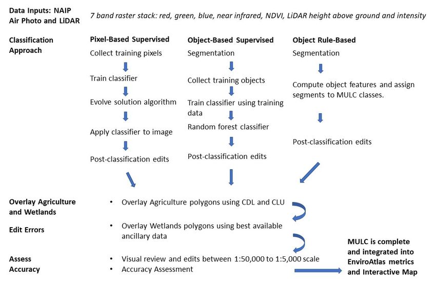
Remote Sens. 2020, 12, 1909                                                                                                4 of 19

      Remote Sens. 2019, 11 FOR PEER REVIEW                                                                               4
      MULC data span the 2010 to 2018 time period. Several datasets are circa 2010 to match the
       intermediate
EnviroAtlas          classes during
               communities      2010 the
                                      US classification
                                          Census focus. stage;
                                                           Thethey
                                                                dateare  providedtofor
                                                                      assigned           potential future
                                                                                      a community’s       analyses
                                                                                                        MULC      data is
       requiring  more  specificity. The   shrub  and  agriculture  classes  are  optional  for a
the predominant year of aerial imagery collection. Metadata indicate if multiple years of imagery  community,     as are
       discussed  below.
used, and year(s) of LiDAR data collection (which are typically not the same as the aerial imagery).
            MULC data span the 2010 to 2018 time period. Several datasets are circa 2010 to match the
      EnviroAtlas Community boundaries are defined by US Census Urban Area Block Groups for
       EnviroAtlas communities 2010 US Census focus. The date assigned to a community’s MULC data is
a Census    Urban Area [5]. An additional 1 km buffer extends outward to eliminate potential edge
       the predominant year of aerial imagery collection. Metadata indicate if multiple years of imagery are
effectsused,
         whenandcalculating  EGS metrics
                  year(s) of LiDAR          based on(which
                                     data collection   moving-window       analyses.
                                                             are typically not  the sameInas
                                                                                           three cases,imagery).
                                                                                             the aerial  we have used
county boundaries
            EnviroAtlasfor   data provided
                         Community            by external
                                       boundaries            partners
                                                    are defined  by US (Chicago,
                                                                        Census Urban IL [comprised     of 10 counties],
                                                                                         Area Block Groups     for a
Los Angeles,     CA, and
       Census Urban   AreaSonoma      County, 1CA).
                            [5]. An additional        The county
                                                 km buffer  extendsis  a convenient
                                                                     outward            geographic
                                                                               to eliminate  potentialunit;
                                                                                                       edge it typically
                                                                                                            effects
leverages
       whencoordinated     geospatial,
              calculating EGS    metrics financial,  and administrative
                                         based on moving-window             resources.
                                                                       analyses.   In three cases, we have used
      county boundaries for data provided by external partners (Chicago, IL [comprised of 10 counties],
2.1. Input Data CA, and Sonoma County, CA). The county is a convenient geographic unit; it typically
      Los Angeles,
      leverages coordinated geospatial, financial, and administrative resources.
     The input raster data stack for EPA-developed MULC typically consists of four-band aerial
photography,
      2.1. Input normalized
                 Data           difference vegetation index (NDVI), and LiDAR data (height above ground
and intensity layers) (Figure 3). Ancillary geospatial data layers (Table 1) are used as available,
            The input raster data stack for EPA-developed MULC typically consists of four-band aerial
advantageous, and appropriate. to overlay agriculture and wetlands on the classified product, and for
      photography, normalized difference vegetation index (NDVI), and LiDAR data (height above ground
performing    post-classification
      and intensity   layers) (Figureerror  correction.
                                        3). Ancillary geospatial data layers (Table 1) are used as available,
     Imagery
      advantageous, and appropriate. toDepartment
                from   the  United   States               of Agriculture
                                             overlay agriculture         (USDA)
                                                                 and wetlands   on National   Agriculture
                                                                                   the classified          Imagery
                                                                                                  product, and
Program     (NAIP)  [6]  is the primary    MULC    aerial
      for performing post-classification error correction.photography.   It has multiple   advantages:
            Imagery from the United States Department of Agriculture (USDA) National Agriculture
•     high  spatial
       Imagery       resolution:
                 Program   (NAIP) 1[6]× is1 the
                                            m pixels
                                                primary(and  fineraerial
                                                          MULC      in some   recent imagery);
                                                                         photography.    It has multiple advantages:
•     free
       •   (no  cost) and   available    for  most  of  the  US;
            high spatial resolution: 1 × 1 m pixels (and finer in some recent imagery);
•      •    free every
      updates    (no cost)
                        twoandtoavailable
                                 three years for most of the US;
                                                 by state;
•      •    updates  every   two  to three   years by state;
      adequate horizontal positional accuracy (≤6 m by specification) (in our experience, NAIP is
       •    adequatewithin
      co-registered    horizontal
                               aboutpositional
                                       two metersaccuracy  (≤ 6 mHR
                                                      of other     by image
                                                                      specification)
                                                                              sources(insuch
                                                                                          our experience,
                                                                                              as Google, NAIP   is co-ESRI);
                                                                                                          Bing and
            registered within about two meters of other HR image sources such as Google, Bing and ESRI);
•     four spectral bands: three visible light bands (blue, green, red) and one near-infrared (NIR) band,
       •    four spectral bands: three visible light bands (blue, green, red) and one near-infrared (NIR)
      which   is used
            band,      to is
                   which   derive   a normalized
                              used to                 difference
                                      derive a normalized          vegetation
                                                               difference       indexindex
                                                                          vegetation     (NDVI).
                                                                                              (NDVI).

      FigureFigure  3. National
               3. National       Agriculture Imagery
                              Agriculture     Imagery Program
                                                        Program  (NAIP)  air photo
                                                                    (NAIP)         and LiDAR
                                                                              air photo         raster band
                                                                                         and LiDAR           stack
                                                                                                         raster    usedstack
                                                                                                                 band
            in MULC    classification. (a) Seven band  raster stack typically used  in MULC   classification,
      used in MULC classification. (a) Seven band raster stack typically used in MULC classification,         plus RGB plus
            and  NIR  for reference. (b) MULC    with 50%  transparency  overlaid  on  NAIP air photo
      RGB and NIR for reference. (b) MULC with 50% transparency overlaid on NAIP air photo showing     showing   region
            of zoomed insets in (a). R (red), G (green), B (blue), NIR (near infrared), NDVI (normalized difference
      region   of zoomed insets in (a). R (red), G (green), B (blue), NIR (near infrared), NDVI (normalized
            vegetation index), HAG (LiDAR height above ground), Intensity (LiDAR intensity), RGB (red-green-
      difference vegetation index), HAG (LiDAR height above ground), Intensity (LiDAR intensity), RGB
      (red-green-blue true color), NRG (NIR-red-green false color composite). Note how different landscape
      features express differently between spectral bands.
Remote Sens. 2020, 12, 1909 5 of 19
NAIP imagery is acquired via internet download or external hard drives from the USDA Aerial
Photography Field Office (APFO) or state sources. The standard data format is uncompressed 8 bit
GeoTIFF with uncalibrated radiance represented by 256 grayscale levels in each band. Uncompressed
data are used to retain maximum spatial and spectral fidelity needed in classification. NAIP images
are typically tiled and distributed using the United States Geological Survey (USGS) 7.5 min quarter
quadrangle topographic map series. A few MULC datasets adapted from external sources may use
other HR aerial imagery as indicated in metadata.
While NAIP imagery is available across the entire conterminous US, airborne LiDAR data are not.
We acquire LiDAR data as available from the USGS National Map [7], NOAA [8], and state and county
geospatial data portals and personnel. LiDAR point clouds are interpolated into rasters of the following
layers: digital elevation model (DEM) (all bare earth, ground points), digital surface model (DSM) (first
point returns), height above ground (HAG) (also referred to as normalized DSM, or nDSM; HAG = DSM
− DEM) and return pulse intensity. (Note: five initial EnviroAtlas communities—Durham, NC, New
Bedford, MA, Paterson, NJ, Portland, ME, and Tampa Bay, FL—were produced without LiDAR).
2.2. Image Classification
EPA-developed MULC data are produced by classifying a raster dataset comprised of NAIP
aerial photos, NDVI and LiDAR HAG and intensity data (Figure 3). Externally developed MULC
datasets are classified from similar raster layers as specified in metadata. We have used three different
classification approaches: pixel-based supervised, object-based supervised, and object rule-based.
The approach used in each community is described in the metadata. Figure 4 shows the overall
workflow for producing MULC data. Pixel-based and object-based classification methods are discussed
in [9]. For MULC datasets created by supervised classification methods, training samples are selected
from within the community boundary being mapped.
Table 1. Primary and supplemental data layers used to generate MULC.
Acronym Dataset Name Comments/Usage
NAIP
National Agricultural 1 m pixel, five band raster stack red-green-blue-near
(Primary data layer used
Imagery Program infrared-NDVI. Approximately three year update cycle.
in classification.)
LiDAR
1 m pixel, two-band raster stack of LiDAR
(Primary data layer used Light detection and ranging
height-above-ground and intensity bands.
in classification.)
Inform algorithms and analysis, 30 m pixel size. Five year
NLCD National Land Cover Dataset
update cycle.
NOAA Coastal Change Inform algorithms and analysis, 30 m pixels. Recently, 1 to
CCAP
Analysis Program 5 m pixel data. Variable update cycle.
National Hydrography Data
NHDPlus v2 Water and wetland feature vectors. Variable update cycle.
Plus Version 2.
NWI National Wetlands Inventory Water and wetland feature vectors. Variable update cycle.
Unattributed parcel polygons emphasizing agriculture.
CLU Common Land Units
Vintage 2008.
Crop information at 30 m pixel size. USDA.
CDL Cropland Data Layer
Updated annually.
Roads and infrastructure Road and utilities data layers Vector data, as available.
Building footprint Building footprint layers Vector data, as available.
The segmentation algorithms used in our object-based classification vary according to the software
used: ArcGIS Desktop (v10.x) [10] and ArcGIS Pro (v2.x) (Segment Mean Shift) [11], ENVI (v5.x)
(Watershed) [12], and eCognition (v9.x) (Multiresolution, Contrast Split) [13]. The analyst prepares
to classify by studying existing land cover information to understand local vegetation, conditions
and landscapes. NLCD and USDA Crop Land Data Layer [14] are particularly useful, in combination
with HR imagery such as Google/Bing/ESRI satellite view, NAIP NIR, Google Street View and Bing
Birdseye view.software used: ArcGIS Desktop (v10.x) [10] and ArcGIS Pro (v2.x) (Segment Mean Shift) [11], ENVI
(v5.x) (Watershed) [12], and eCognition (v9.x) (Multiresolution, Contrast Split) [13]. The analyst
prepares to classify by studying existing land cover information to understand local vegetation,
conditions and landscapes. NLCD and USDA Crop Land Data Layer [14] are particularly useful, in
combination
Remote Sens. 2020,with HR imagery such as Google/Bing/ESRI satellite view, NAIP NIR, Google Street
12, 1909 6 of 19
View and Bing Birdseye view.
Figure 4.4. MULC
MULCclassification workflow.
classification MULC data
workflow. MULC are data
createdareusing one of
created threeone
using classification
of three
methods. Abbreviations
classification methods. are defined in the
Abbreviations aretext. Land cover
defined in thedatasets created
text. Land by external
cover datasetspartners
created are
by
recoded
external to EnviroAtlas
partners MULCtoclasses
are recoded and run
EnviroAtlas MULCthrough the and
classes post-classification
run through the steps (overlay, edit,
post-classification
assess).
steps (overlay, edit, assess).
2.3. Post-Classification
2.3. Post-Classification Operations
Operations
2.3.1. Post-Classification Operations
2.3.1. Post-Classification Operations
The MULC data are reviewed after classification and errors are addressed in two ways. First,
The MULC data are reviewed after classification and errors are addressed in two ways. First, we
we perform as many edits as possible using GIS functions (e.g., conditional statements, convolution
perform as many edits as possible using GIS functions (e.g., conditional statements, convolution
filtering). Ancillary spatial layers such as roads and building footprints are useful to mask and focus
filtering). Ancillary spatial layers such as roads and building footprints are useful to mask and focus
edits. We inspect each output layer to detect potential artifacts introduced by post-classification GIS
edits. We inspect each output layer to detect potential artifacts introduced by post-classification GIS
functions. Second, we perform manual editing (on-screen, heads-up digitizing) to identify and recode
functions. Second, we perform manual editing (on-screen, heads-up digitizing) to identify and recode
remaining errors. Here the analyst interactively selects pixel groups (or polygons) for recoding from the
remaining errors. Here the analyst interactively selects pixel groups (or polygons) for recoding from
incorrect to correct class. Manual editing is labor intensive and time consuming but can substantially
the incorrect to correct class. Manual editing is labor intensive and time consuming but can
improve the visual appearance.
substantially improve the visual appearance.
2.3.2. Fuzzy Accuracy Assessment
2.3.2. Fuzzy Accuracy Assessment
We use a fuzzy approach [15] to assess the accuracy of the MULC classification. The motivation is
to better accommodate the non-exclusive nature of land cover class membership: “The need for using
fuzzy sets arises from the observation that all map locations do not fit unambiguously in a single map category.
Fuzzy sets allow for varying levels of set membership for multiple map categories. A linguistic measurement scale
allows the kinds of comments commonly made during map evaluations to be used to quantify map accuracy” [15].
An assessment analyst labels the land cover at each reference point (pixel) and assigns a fuzzy
confidence value to the label on a scale from (1) (incorrect) to (5) (correct). For example, tree canopy
over grass is a situation where both classes could be considered “correct”. The sensor may capture both
the canopy and the ground through thin canopy or canopy gaps. The analyst might assign a tree label
with confidence of 4, and a grass label with a confidence of 3. Another situation is accommodating
the continuum between grass and soil endmembers. The fuzzy approach allows both agriculture
and soil class labels to be considered correct for a barren crop field. Accuracy assessment results are
presented in two confusion (error) matrices, showing errors of omission (producer’s accuracy) andRemote Sens. 2020, 12, 1909 7 of 19
errors of commission (user’s accuracy) for each class as well as an overall accuracy value. The fuzzy
confusion matrix is less conservative and based on these fuzzy confidence evaluations; the non-fuzzy
confusion matrix is more conservative and based on strict binary correct/incorrect class membership.
The MULC classification is compared to 500 to 700 randomly distributed photo interpreted
reference points (i.e., an initial target of 100 reference points per class, 5 to 7 classes per community).
If rare classes (e.g., soil, water) are under-sampled (n < 50), additional reference points are collected
to reach n ≥ 50, stratified by class as indicated by the MULC classification. The NAIP imagery input
to the classification serves as the primary photo interpreted reference imagery. This assures spatial
and temporal correspondence of the reference imagery and the MULC classification. Uninterpretable
or ambiguous points may be removed from consideration (e.g., deep shadow or boundary between
classes). Photo interpretation is aided by spatially linked displays of LiDAR-derived layers, NIR
false color composite and other temporally appropriate high resolution imagery as noted above.
Wetland classes (woody and emergent) are not included in the accuracy assessment. Because remote
identification of wetlands is complex and beyond the scope of our study, we assume that the ancillary
wetlands data are reliable. However, reference pixels located in wetland areas are assessed in terms of
their non-wetlands, underlying MULC class.
The final quality assurance step is on-screen visual assessment of the classified MULC by multiple
analysts at scales from 1:50,000 to 1:5000. Known errors and uncertainties are described in the metadata
for each community.
2.4. Definitions of MULC Classes
The standard EnviroAtlas MULC product is provided at a “Level 1” thematic resolution and is
similar but not identical to the Anderson and NLCD Level 1 classes (Table 2) [3,16]. MULC data are
published at Level 1; a structure of Level 2 classes is provided below in anticipation of potential future
analyses requiring greater thematic specificity.
As discussed above, data are either created by EPA EnviroAtlas personnel or incorporated from
external non-EPA sources. Externally produced data must meet these criteria:
• The classes can be unambiguously translated to the MULC system;
• The data are at same or finer spatial resolution;
• The data are sufficiently contemporaneous with the EnviroAtlas period of study;
• The data have an overall target fuzzy accuracy ≥80%. (We perform the standard MULC accuracy
assessment on externally developed LC data.)
To the first point, a dataset acquired from external sources that contains separate building and
street classes can be unambiguously recoded into the MULC Impervious Surface class. However,
a hypothetical residential class defined as “50% impervious surface and 50% vegetation” cannot be
used because impervious, trees, shrubs and grass are inseparably combined into a single class and
cannot be unmixed.Remote Sens. 2020, 12, 1909 8 of 19
Table 2. MULC Level 1 and 2 class names, codes, and descriptions.
Standard MULC
Level 1 Code Level 2 Codes Short Description
Level 1 Class
The water class includes all natural
11 Fresh Water and some anthropogenic surface
12 Salt Water waters: rivers, streams, canals,
Water 10 Water
13 (available) ponds, reservoirs, lakes, bays,
14 Drinking Water Reservoir estuaries, and near-shore
coastal waters.
The impervious class includes
21 Dark Impervious
buildings, paved roads, parking lots,
(low reflectance)
driveways, sidewalks, roofs,
22 Light Impervious
swimming pools, patios, painted
(high reflectance)
surfaces, wooden structures, solar
Impervious Surface 20 Impervious Surface 23 Road
farms and most asphalt and
24 Building
concrete surfaces. Swimming pools,
25 Parking Area
and wastewater treatment tanks and
26 Soil and Gravel Impervious
basins, are labeled as Impervious as
27 Solar Panel
described in the text.
The soil and barren class (“soil”)
includes bare soil, bare rock, mud,
clay, sand, barren agricultural fields
31 Developed Soil (soil in
(for communities with less than 5%
developed areas likely
agriculture), construction sites,
compacted and disturbed)
Soil-Barren 30 Soil and Barren Land quarries, gravel pits, mine lands,
32 Bare Rock
industrial land, parking lots, golf
33 Sand and Gravel
course sand traps, ball parks,
34 Quarry
playgrounds, stream and river sand
bars, sand dunes, beaches and other
bare soil and gravel surfaces.
Woody single stem vegetation ≥ 2 m
height. “tall vegetation.” Generally,
the branching starts above a
specified trunk height, in contrast
41 Deciduous Tree/Forest
with shrubs where branching starts
42 Evergreen Tree/Forest
near ground level. Classes 45–47 are
43 Mixed Tree/Forest
optional and subordinate to height
Tree 40 Tree 45 Low Tree (height < 2 m)
thresholds defined in the text.
46 Medium Tree
The term Tree comprises trees of
(2 m ≤ height < 5 m)
varying extent: individual trees,
47 High Tree (height ≥ 5 m)
stands and forest. The codes 41–47
are provided as guidelines for
potential future analyses; they have
not been used in MULC data to date.
51 Shrubland or Scrubland
(undifferentiated Shrub,
Soil and Grass)
Woody multiple stem vegetation
52 Individual Shrub in Natural
with height ≤ 2 m and > 0.5 m.
Environment
“medium height vegetation.”
Shrub 50 Shrubs or Shrubland 53 Individual Shrub in
Shrub mapping requires LiDAR
Built/Developed Environment.
height above ground except in
55 Low Shrub (height ≤ 2 m)
known shrub land areas.
56 Medium Shrub
(2 m < height < 5 m)
57 High Shrub (height ≥ 5 m)
Graminoids, forbs and herbs lacking
persistent woody stems; includes
residential lawns, golf courses,
71 Lawns and Other
roadway medians and verges, park
Managed Grass
lands, transmission line and natural
72 Roadside Grass
Grass-Herbaceous 70 Grass gas corridors, recent forest
73 Pasture
clear-cuts, meadows, pasture,
74 Natural Grassland
grasslands and prairie grass. Also
(e.g., prairie)
known as “low vegetation.” Grass
classified in wetlands areas is
recoded to emergent wetlands.Remote Sens. 2020, 12, 1909 9 of 19
Table 2. Cont.
Standard MULC
Level 1 Code Level 2 Codes Short Description
Level 1 Class
Row crops (80) and orchards (82)
(Note: agriculture class numbering
80 Row Crops departs from the norm.) Pixels
Agriculture 81 Agriculture
82 Orchard classified as grass (70) are recoded
to row crop (80) when the ancillary
agricultural polygons are overlaid.
Emergent (91) and woody
(92) wetlands
Wetlands polygons are overlaid on
classified MULC using best
91 Emergent Wetland available data (e.g., NWI, NHD+).
Wetlands 90 Wetlands
92 Woody Wetland Grass recodes to emergent wetland.
Trees recode to woody wetland. Soil,
water and impervious classes
remain unchanged. Treatment of
shrubs is indicated in metadata.
2.4.1. Unclassified
The 00 unclassified class is available for special cases or unanticipated LC classes not present in
the existing MULC system.
2.4.2. Water
The water class includes all natural and some anthropogenic surface waters: rivers, streams,
canals, ponds, natural lakes, artificial lakes, dammed valley reservoirs, bays, estuaries and near-shore
coastal waters. Note that wastewater treatment tanks, clarifiers, basins and sumps are labeled
impervious surfaces, as are swimming pools, fountains and similar small anthropogenic water features.
This distinction is made based on their ecosystem services which are very different to those in the
forms of surface water above: they are not biologically active (wastewater treatment notwithstanding);
they are closed systems without natural surface water exchange with the environment; they are
constructed features. The water class is most commonly confused with shadow, trees and dark
impervious surfaces. Bright sun glint on water is confused with highly reflective classes such as soil
or impervious surface. Turbid, sediment-laden brown or tan water is confused with soil. Shallow
water is confused with soil, impervious and vegetation depending on bottom surface optics of the
substrate (e.g., sand, silt, rock, submerged vegetation). Water with floating vegetation may misclassify
as vegetation but is intended to be in the water class. Floating vegetation is assumed to be ephemeral,
and that the LC at such a point is better represented as water than vegetation.
Lakes, ponds, tidal zones, estuaries and other water bodies that vary in extent and shoreline
location over time are mapped according to how they appear in the imagery; i.e., at the date and time
of image acquisition. If circumstances favor using a different shoreline (e.g., authoritative NOAA
shoreline) this is indicated in the metadata.
2.4.3. Impervious Surface
An impervious surface prevents or substantially limits rainfall and other water from infiltrating
into the soil. The impervious class includes paved roads, parking lots, driveways, sidewalks, roofs,
swimming pools, patios, painted surfaces, wooden structures and most asphalt, concrete and paved
surfaces. In MULC, dirt roads, gravel roads and railways are classified as impervious. These areas
are compacted, disturbed and altered leading to a loss of perviousness. Except for bare rock, most
impervious surfaces are anthropogenic and most pervious surfaces are natural (e.g., vegetation, soil).
Bare rock is functionally impervious and is commonly confused spectrally with the impervious class,
but in MULC it is assigned to the soil and barren class. Rooftops and roads that incorporate sand and
clay materials are spectrally confused with soil but belong in the impervious class.Remote Sens. 2020, 12, 1909 10 of 19
Level 1 MULC combines roads/pavements and buildings into one impervious class (20), rather
than separate Level 2 roads (23) and buildings (24) because of the requirement for height information
to classify buildings. The original MULC classes are designed to be classified from NAIP imagery,
with or without LiDAR, because of patchy LiDAR availability. If height above ground or building
footprints are available, one can separate roads and buildings.
Solar panel farms (class 27) are a separate impervious Level 2 class. They represent a third type of
impervious built surface after pavements and buildings/rooftops. Solar panels present an interesting
EGS case in that biological functions continue beneath the artificial canopy. The panels provide shade
and collect and distribute rain preferentially.
2.4.4. Soil-Barren
The soil and barren class (“soil”) includes soil, bare rock, mud, clay, sand, barren (fallow)
agricultural fields, construction sites, quarries, gravel pits, mine lands, recreational areas, golf course
sand traps, ball parks, playgrounds, stream and river sand bars, sand dunes, beaches and other bare
soil, sand, gravel and rock surfaces. Soil and barren includes natural areas with widely spaced or no
vegetation cover, including the soil substrate of semiarid and arid rangeland, shrubland and desert.
Unpaved dirt roads, gravel roads, and railways are typically semi-impervious, and are assigned to the
impervious class unless otherwise noted.
Soil is a relatively rare class in humid temperate communities such as Milwaukee, WI, Pittsburgh,
PA and Portland, ME. Soil is more common in arid communities such as Phoenix, AZ and Fresno,
CA. Construction sites are a common soil surface in highly developed urban landscapes, and barren
agricultural fields on the periphery. Soil is commonly confused with light impervious surfaces.
2.4.5. Tree
The tree class includes trees of any kind, from a single individual to continuous canopy forest.
Trees are single stem woody perennial plants with a trunk, branches and leaves and height greater than
2 m. Signature characteristics of the tree class in NAIP imagery include greenness, high NIR reflectance,
NDVI, a mottled textured canopy, tree crowns illuminated and shadowed on opposite facets, visible
trunks, length of shadows and context. Signature characteristics of the tree class in LiDAR include
height above ground, intensity, object shape, multiple LiDAR returns and canopy surface texture.
Level 1 MULC combines deciduous and evergreen trees in one tree class. Shrubs greater than
two meters height are classified as tree unless otherwise indicated. Bamboo is botanically a grass
(family Poaceae) but is classified as tree here if height ≥ 2 m. Trees are most commonly confused with
water, dark impervious, shrub and grass.
Tree canopy pixels that extend over other LC surfaces such as streets, buildings and lawns are
assigned to tree rather than the underlying class. The tree canopy is what the sensor “sees” in its direct
line of sight. This convention reflects an EnviroAtlas emphasis on EGS and the importance of street
trees in urban areas. Thus, where trees extend over a road, driveway, sidewalk or rooftop, the amount
of underlying impervious surface (or grass, soil or water) will be underestimated. The horizontal
surface area of tree canopy will be correctly estimated. If accurate road and building footprint data are
available, one may compute the under-canopy extent of these obscured surfaces.
2.4.6. Shrub
Shrubs are multiple stem woody perennial plants between 0.5–2 m height. Shrubs are recognized
in air photos by context (e.g., desert, rangeland, urban landscaping), the mottled texture of the
canopy (compared to grass), and lesser shadows (compared to trees). Shrubs are recognized by height
(and possibly shape) in LiDAR data.
In some land cover datasets, arid and semiarid natural shrub vegetation is mapped as
undifferentiated shrubland (51). In that case, shrubs, soil, and grass are mixed in a single class,
rather than as differentiated classes of shrub (52), grass (70) and soil (30). In EnviroAtlas, using shrubRemote Sens. 2020, 12, 1909 11 of 19
class (52) (individual shrubs) is preferred over shrubland (51). Shrub (52) is at a finer information
granularity to support EGS analysis.
2.4.7. Grass-Herbaceous
The grass and herbaceous class (“grass”) includes the graminoids, forbs and herbs lacking
persistent woody stems. Grass includes residential lawns, golf courses, roadway medians and
verges, park lands, transmission line and natural gas corridors, recently clear-cut forest areas, pasture,
grasslands, and prairie grass. Small shrubs may fall into this category as noted above. It is also known
as “low vegetation.”
For healthy, photosynthetically active grass, the principal identifying characteristics in NAIP
imagery are greenness, high reflectance in the near infrared, high NDVI, urban context and a smoother
image texture than tree and shrub canopy. Context helps in identifying grass (e.g., proximity to
a building, athletic field or highway). NAIP imagery is collected in summer leaf-on conditions
when grass may be green, or brown with heat and moisture stress. Sparse or brown grass is
commonly confused with soil and impervious surfaces. Grass-soil confusion is greater in arid than in
humid-temperate environments.
What to do with indeterminate pixels in NAIP imagery that could be either grass or soil?
Sparse, brown or dead grass are spectrally like soil, and soil and grass intermix along a continuum.
As a guideline, if potential grass or soil pixels/polygons show above-background reflectance in the
near-infrared band (indicative of photosynthetic activity), they are labeled grass. An operational
assumption is that, except in arid regions, soil has the potential to support grass or other vegetation at
some point during the growing season. The analyst consults other HR imagery from different dates to
assess if grass is present at other times.
2.4.8. Agriculture
Agriculture is a layer superimposed on the MULC classification. The USDA Common Land
Unit (polygon) [17] and raster Cropland Data Layer (CDL) [14] are used to help identify agriculture
polygons. Level 2 Agriculture is labeled as row crops (80) if MULC pixels are classified as grass,
shrub, or soil and fall within these ancillary agricultural datasets, and orchards (82) if classified as
tree. (Note: the agriculture class numbering deviates slightly from standard MULC class numbering
conventions due to a transcription error in the initial data upload). Pasture is assigned to the grass
class for two reasons: (1) difference in land management practices between row crops and pasture, and
(2) difficulty differentiating pasture from non-cultivated grass.
The agriculture (“Ag”) class is included in a MULC product if the most recent NLCD indicates
agriculture greater than 5% within the EnviroAtlas community boundary. If agriculture is less than or
equal to 5%, agriculture pixels (polygons) are labeled as whatever LC is on the ground when the NAIP
imagery is acquired (grass, soil, shrub or tree), rather than as agriculture. Twenty of the EnviroAtlas
communities have an agriculture class.
2.4.9. Wetlands
As defined by Section 404 of the Clean Water Act: “Wetlands are areas that are inundated or
saturated by surface or ground water at a frequency and duration sufficient to support, and that under
normal circumstances do support, a prevalence of vegetation typically adapted for life in saturated soil
conditions” [18]. Wetlands include swamps, marshes, bogs, and other wet and flooded areas [19,20].
Like agriculture, in MULC data, wetlands are delineated using the best available ancillary data,
which to date have been the U.S. Fish and Wildlife Service National Wetlands Inventory (NWI) [21]
and U.S.G.S. National Hydrography Dataset (NHDPlus v2) [22]. Classifying wetlands directly from
imagery/LiDAR is beyond the scope of this study, and generally requires ground validation and
ancillary data. Wetlands boundary polygons are overlaid on the MULC data; areas classified as tree
are labeled woody wetland (91), and areas classified as grass-herbaceous are labeled emergent wetlandRemote Sens. 2020, 12, 1909 12 of 19
(92). Treatment of shrub areas is indicated in the community metadata. Visual checks are performed
for thematic and positional agreement of wetlands layers and underlying imagery.
3. Results
Here we present statistics characterizing the MULC dataset. Table 3 summarizes the size,
population, year and accuracy statistics for 30 EnviroAtlas communities. MULC communities
range considerably in both aerial extent and population, with the largest community (Chicago)
encompassing more than 14,000 km2 and the smallest (Paterson, NJ) spanning just 47 km2 . The mean
area is 3139 km2 . Community populations closely aligned with aerial extent in a positive relationship.
The largest community population is over 9.8 million (Los Angeles, CA County, 11,336 km2 ) and
the smallest is just over 1500 people (Woodbine, IA, 51 km2 ). The mean population for EnviroAtlas
communities is 2.1 million people according to the 2010 U.S. Census [23].
Table 3. MULC statistics for EnviroAtlas communities. Abbreviations after the community name
indicate the main method used in classification: pixel-based supervised (PBS), object-based supervised
(OBS), or object rule-based (ORB).
Population Overall Overall
EnviroAtlas Area Kappa Kappa Imagery LiDAR
(2010 Accuracy Accuracy
Community (km2 ) (Fuzzy) (Non-Fuzzy) Date Dates
Census) (Fuzzy) (Non-Fuzzy)
Austin, TX (PBS) 2499 1,334,516 90.7 87.9 86.5 82.6 2010 2007
2004,
Baltimore, MD 2005,
4545 2,252,753 92.7 90.5 90.1 87.1 2013
(ORB) 2011,
2015
2010,
Birmingham, AL
2335 763,628 87.6 80.5 83.4 74.2 2011 2011,
(PBS)
2013
Brownsville, TX 2011,
938 223,572 82.3 77.6 76.7 70.6 2014
(PBS) 2006
2006,
2007,
2010, 2012, 2008,
Chicago, IL (ORB) 14,687 9,203,201 86.8 83.6 80.8 76.0
2013 2010,
2013,
2014
Cleveland, OH
2737 1,758,114 90.2 86.9 86.2 81.6 2011, 2013 2006
(PBS/ORB)
1 m for
2008, 2009;
Des Moines, IA
1130 456,017 84.6 80.4 77.6 73.5 0.61 m for 2009
(PBS)
2007, 2009,
2010
Durham, NC (PBS) 569 340,851 N/A N/A 83.0 78.8 2010 N/A
Fresno, CA (PBS) 753 659,628 86.9 83.5 81.1 76.2 2010 2012
Green Bay, WI (PBS) 857 219,947 94.1 92.7 90.4 87.9 2010 2010
Los Angeles County
11,336 9,818,599 89.2 86.2 61.1 53.4 2014, 2016 2016
(ORB)
2009,
2010,
Memphis, TN (PBS) 2516 1,091,638 89.0 86.1 86.9 83.5 2012, 2013
2011,
2012
Milwaukee, WI
2154 1,373,711 85.5 80.5 76.2 68.9 2010 2010
(ORB)
Minneapolis/St.
3085 2,282,061 87.7 84.4 87.1 83.6 2010 2011
Paul, MN (ORB)
New Bedford, MA
258 151,164 95.0 93.0 92.3 89.2 2010 N/A
(PBS)
2006,
New Haven, CT
1422 578,536 92.0 88.8 89.0 83.2 2014 2010,
(PBS)
2011Remote Sens. 2020, 12, 1909 13 of 19
Table 3. Cont.
Population Overall Overall
EnviroAtlas Area Kappa Kappa Imagery LiDAR
(2010 Accuracy Accuracy
Community (km2 ) (Fuzzy) (Non-Fuzzy) Date Dates
Census) (Fuzzy) (Non-Fuzzy)
New York, NY
1109 8,175,131 87.4 83.2 84.2 79.0 2011 2010
(ORB)
Paterson, NJ (PBS) 47 146,199 92.5 89.2 86.8 81.2 2010 N/A
Philadelphia, PA 2005–2008, 2006–2008,
7184 5,425,378 86.4 82.3 77.6 70.6
(ORB) 2012–2015 2011–2015
Phoenix, AZ (ORB) 5406 3,704,874 75.4 65.9 69.2 57.7 2010 N/A
Pittsburgh, PA (PBS) 1927 1,209,128 89.3 85.1 86.5 81.3 2010 2006
Portland, ME (PBS) 523 191,292 N/A N/A 87.5 85.0 2010 N/A
2007,
Portland, OR (PBS) 2507 1,853,233 91.4 89.2 78.5 73.5 2011, 2012
2010
2006–2007,
Salt Lake City, UT
2244 1,030,599 82.5 77.0 78.7 72.0 2014 2011,
(ORB)
2013–2014
Sonoma County, CA
4910 483,878 80.9 75.8 79.0 73.4 2011,2013 2013
(OBS)
2012, 2008–2010,
St. Louis, MO (OBS) 4188 2,174,437 90.4 87.9 82.3 77.7
2014–2016 2012
Tampa, FL (PBS) 4492 2,517,798 N/A N/A 70.6 65.2 2010 N/A
2015,
Virginia Beach, VA
3255 1,541,779 84.1 80.6 83.5 79.9 2013, 2014 2010,
(OBS)
2013
2004,
2008,
Washington, DC 2011,
5423 4,693,748 91.5 88.7 85.4 80.6 2013, 2014
(ORB) 2012,
2015,
2016
Woodbine, IA (PBS) 51 1555 90.2 84.4 87.0 79.3 2011 2009
Mean 3170 2,188,566 88.0 84.0 82.0 77.0
Total 95,088 65,656,965
N/A means data not available for this community. Fuzzy accuracy assessment was implemented after the first three
communities were created and not retroactively performed.
The data used for classification in each community vary by availability, and typically the most
recent available data are prioritized. Twelve of the 30 communities published to EnviroAtlas are based
on 2010 NAIP imagery and most of the other communities are based on NAIP imagery from 2016 or
earlier (Table 3). Twenty-four community datasets incorporate LiDAR, but, due to the timing of LiDAR
acquisition, only four of those communities have LiDAR matching the imagery collection dates. LiDAR
is not collected as frequently as imagery, and collection years for both LiDAR and imagery often do not
overlap. When imagery and LiDAR are of different dates and do not agree due to land use changes,
the analyst typically defers to the imagery when making post-classification corrections and during the
accuracy assessment process. Data limitations for each community are indicated in metadata.
Table 4 summarizes fuzzy and non-fuzzy MULC accuracies by class for all existing EnviroAtlas
communities. Table 5 is a confusion matrix constructed from 17,760 reference points for the
27 EnviroAtlas communities that have received both fuzzy and non-fuzzy accuracy assessments,
illuminating the nature of interclass confusion.Remote Sens. 2020, 12, 1909 14 of 19
Table 4. MULC mean class accuracies across 30 EnviroAtlas communities.
Agriculture Grass Impervious Shrub Soil Tree Water
Fuzzy User Accuracy 90.4 82.6 90.8 79.7 76 86.9 96.1
Fuzzy Producer
94.8 78.5 85.7 80.9 82.4 88.6 95.7
Accuracy
Non-Fuzzy User
82.5 75.1 87.8 71.6 63.2 83.5 95.3
Accuracy
Non-Fuzzy Producer
82.6 68.7 83.3 71.7 73.8 85.3 94.2
Accuracy
Class user and producer accuracies for all communities are generally high and increase between
non-fuzzy and fuzzy assessments (Table 4). The class user accuracy, calculated by dividing the number
of correct reference points (where both the row and column classes agree) for a class by the row total,
indicates how well the land cover represents the class as defined by the reference points. The class
producer accuracy, calculated by dividing the number of correct reference points for a class by the
column total, indicates how well the class is represented in the classification. The most accurate class
in MULC landcover is water. Twenty-eight communities have both fuzzy and non-fuzzy accuracy
assessments. The mean overall accuracy across all EnviroAtlas communities is 88% fuzzy and 82%
non-fuzzy. Overall fuzzy accuracy is always higher than overall non-fuzzy accuracy. Mean kappa
values are 0.84 fuzzy and 0.77 non-fuzzy. The soil class has the lowest user accuracy (77.8%) and
grass class has the lowest producer accuracy (78.9%). Based on the fuzzy confusion matrix (Table 5),
grass class confusion is mostly with soil and tree classes.
Table 5. Fuzzy confusion matrix for n = 27 communities.
Reference Classes
Agriculture Grass Impervious Shrub Soil Tree Water Row Total User Accuracy
Agriculture 1771 108 4 1 39 10 1 1934 0.92
Grass 19 3100 192 16 98 280 15 3720 0.83
Land Impervious 2 111 2761 2 86 59 8 3029 0.91
cover Shrub 3 46 20 441 24 11 0 545 0.81
Classes
Soil 27 198 117 23 1446 24 24 1859 0.78
Tree 5 351 129 29 21 4359 13 4907 0.89
Water 0 17 8 0 22 12 1707 1766 0.97
Column
1827 3931 3231 512 1736 4755 1768 17760
Total
Producer
0.97 0.79 0.86 0.86 0.83 0.92 0.97
Accuracy
Overall
Fuzzy 0.88
Accuracy
Kappa 0.85
Three early communities are omitted because they lack a fuzzy accuracy assessment: Durham, NC; Portland, ME;
Tampa, FL.
Soil class mixing is mostly with grass and impervious. Shrub landcover class is mapped in only
six (western) communities and consequently has fewer reference points than the other classes.
4. Discussion
MULC underpins metrics that complement those derived from the national, 30 m resolution land
cover component in EnviroAtlas, offering decision makers, researchers and others the ability to evaluate
ecosystem services and land cover characteristics at household/street, community, neighborhood (block
group), city, and regional levels. MULC and other EnviroAtlas data have been used in a range ofRemote Sens. 2020, 12, 1909 15 of 19
applications from regional to local scales. In Portland, Oregon, city planners have used MULC to
design street tree planting and green infrastructure for urban heat island mitigation [24]. In Durham,
North Carolina, EnviroAtlas has been used to identify census block groups with low tree cover and
vulnerable populations to explore how tree planting might benefit child development, overall public
health, and environmental quality [25,26]. In Tampa Bay, Florida, a Health Impact Assessment (HIA)
has demonstrated how MULC and EnviroAtlas metrics, tools, and data can assist decision makers
in a health and wellness application [27]. See the EnviroAtlas use case page for more information
(https://www.epa.gov/enviroatlas/enviroatlas-use-cases).
The high level of detail provided by MULC data contributes to diverse research, ranging from
environmental and public health to the economic benefits attributed to EGS. MULC data and derived
EnviroAtlas community metrics support research including epidemiological studies on the salutogenic
effects of natural environment exposure in urban areas [28], mosquito distribution analyses to assess
vector-borne disease risk in Texas [29], and urban revitalization efforts in the Great Lakes region [30],
among others. A bibliography of research using MULC and other EnviroAtlas data can be found on
the EPA EnviroAtlas website: https://www.epa.gov/enviroatlas/enviroatlas-publications.
4.1. Uncertainty in MULC Data
In this section, we discuss MULC interpretation and origins of common uncertainties in MULC
data. It is important that map classification errors be understood so that the EGS metrics can be
accurately estimated, as major map errors can translate into incorrect valuation of ecosystems [31].
A confusion matrix is just one expression of map accuracy and users have varying needs that may
prioritize map characteristics other than the statistical evaluation of reference points. MULC datasets
have been developed using both pixel-based and object-based methods and land cover features,
in actuality, are groupings of pixels representing the real world. MULC users who reside in the
communities represented in the MULC dataset series are likely to possess the best understanding of
accurate (or expected) land cover types in the areas of interest. There are times when a map can have
high statistical accuracy but still possess errors in a particular area of local interest; this can make
users lose confidence in the product. It is important that a map has good statistical accuracy, but also
accurately represents real conditions for local users. It is for that reason that we spend a large portion
of the data development process in quality assurance (QA) to ensure that MULC datasets possess
acceptable statistical accuracies and have minimal visual errors.
4.2. Evaluation and Uncertainty in MULC
We recommend that to evaluate MULC data, the user display MULC at 40–60% transparency
overlaid on the source imagery (e.g., NAIP) basemap and view at multiple zoom levels. This allows
direct comparison of the MULC layer and source imagery. Comparing with higher resolution
(e.g., 0.1–0.5 m) imagery may add additional useful information. Displaying the MULC over a more
recent image basemap may visually highlight sites of land cover change.
There are multiple types of uncertainty and errors in high resolution land cover data for
consideration when evaluating data accuracy and quality:
1. True misclassification (e.g., the image pixel is composed of soil but the map labelled it grass);
2. Non-exclusive class membership (the pixel is a mixture of soil and grass);
3. Inter-observer error (the map developer and the accuracy assessor use different criteria (e.g., pixel
color and brightness) for labeling an ambiguous pixel as either soil or grass)
4. Severity of misclassification (for a specific user application, mistaking grass for tree may be
less significant than mistaking soil for tree [i.e., vegetated versus non-vegetated] or water for
impervious);
5. Items 2 and 3 are allowed greater flexibility as a result of the fuzzy accuracy assessments employed
for MULC datasets.You can also read