Validation of the Westinghouse BWR nodal core simulator POLCA8 against Serpent2 reference results - MATHILDE GAILLARD
←
→
Page content transcription
If your browser does not render page correctly, please read the page content below

EXAMENSARBETE INOM TEKNISK FYSIK,
AVANCERAD NIVÅ, 30 HP
STOCKHOLM, SVERIGE 2021

Validation of the Westinghouse
BWR nodal core simulator
POLCA8 against Serpent2
reference results

MATHILDE GAILLARD

KTH
SKOLAN FÖR TEKNIKVETENSKAP

Validation of the Westinghouse BWR
  nodal core simulator POLCA8 against
        Serpent2 reference results

                          Mathilde Gaillard

Date: February, 2021
Degree Project in Engineering Physics (30 ECTS credits)
Double engineering degree between Grenoble INP Phelma and KTH Royal Institute of
Technology
Supervisor at KTH: Vasily Arzhanov
Examiner at KTH: Prof. Jan Dufek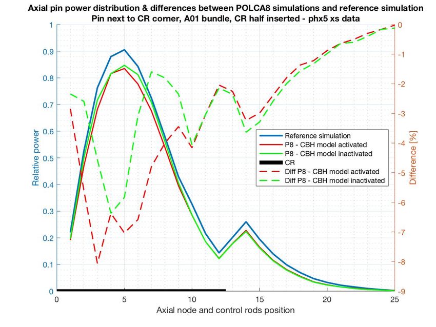
Mathilde Gaillard, MSc                                            Master Thesis Report

TRITA-SCI-GRU 2021:018

Royal Institute of Technology
School of Engineering Sciences
KTH SCI
SE-100 44 Stockholm, Sweden URL: www.kth.se/sci

Westinghouse Eletric Sweden AB, Västerås, Sweden, February 2021                     ii

Mathilde Gaillard, MSc                                                                    Master Thesis Report

Aknowledgement
    First of all, I would like to thank Mr Jan Dufek, one of my teacher at KTH, for helping me to find this
master thesis thanks to his contacts, as well as I would like to thank Mr Jean-Marie Le Corre, the first person I
met from Westinghouse, for helping me to find an interesting topic in the field I am most interested in within
the company, and Mr Magnus Limbäck, for helping me with the technical details once I was accepted for this
master thesis.

    I would also like to thank and express my gratitude to Mr. Petri Forslund Guimarães for accepting me into
the project and taking me on as a student. He spent a lot of time teaching me all the important aspects of the
subject, and we had many interesting conversations about how to solve the problems we were facing. He was
also very helpful with his comments on how to write the thesis correctly, and I know that all the lessons he
taught me will be useful to me throughout my career.

   I would like to thank Mr Vasily Arzhanov for advice on how to write this master thesis.

    I would also like to thank my friends and coworkers from KTH with whom we helped each other during
this particular period of teleworking and kept ourselves motivated during the whole thesis period. I am thinking
in particular of one of my closest friends, Dr Benjamin Portal, who supported me both morally and technically
with his advice on graphics and writing.

   Finally, I would like to thank all the people who have helped me, or who have helped to make the project a
success, in one way or another.

   A special thought belongs to my father, who, I know, from where he is, would have been really proud of me.

Westinghouse Eletric Sweden AB, Västerås, Sweden, February 2021                                                ii
Mathilde Gaillard, MSc                                                                        Master Thesis Report

Abstract
    When a new nodal core simulator is developed, like all other simulators, it must go through an extensive
verification and validation effort where, in the first stage, it will be tested against appropriate reference tools in
various theoretical benchmark problems. The series of tests consist of comparing several geometries, from the
simplest to the most complex, by simulating them with the nodal core simulator developed and with some higher
order solver representing the reference solution, in this case on the Serpent2 Monte Carlo transport code. The
aim of this master’s thesis is to carry out one part of these tests. It consisted in simulating a three-dimensional
(3D) 2x2 mini boiling water reactor (BWR) core with the latest version of the Westinghouse BWR nodal core
simulator POLCA8, and in comparing the outcome of these simulations against Serpent2 reference results.
Prior to this work, POLCA8 was successfully tested on a 3D single-channel benchmark problem using the same
Serpent2/POLCA8 methodology. However, this benchmark problem considered in this work is challenging in
several aspects. Indeed, the nodal core simulator should accurately predict the eigenvalues and power distribu-
tions against reference results, and this by taking into account axial leakage, resulting from the passage from
two-dimensional (2D) infinite lattice physics calculations to 3D simulations, or strong axial flux gradients due to
the insertion or withdrawal of the control rods after a certain depletion. This last effect is known as the Control
Blade History (CBH) effect and will be the main focus of this study. In addition to the development of a new
version of the nodal core simulator, a new version of the Westinghouse deterministic transport code PHOENIX5
is also under development. The accuracy of PHOENIX5 was indirectly tested through this benchmark by
providing the cross sections for the POLCA8 simulations. In addition, Serpent2 based nodal cross sections were
generated to POLCA8 to provide means of comparing these two sets of nodal cross section data. The results
obtained lead to the conclusion that the CBH model gives very good results, especially with regard to all power
distributions, and especially those after the removal of the control bars when needed most.

    keywords: Nodal Core Analysis, Monte Carlo Methods, CBH Effects

Westinghouse Eletric Sweden AB, Västerås, Sweden, February 2021                                                    iii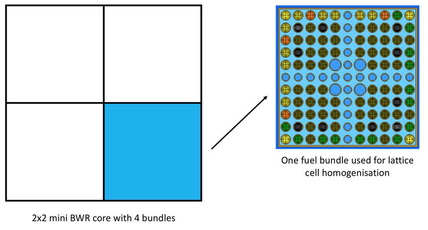
Mathilde Gaillard, MSc                                                                    Master Thesis Report

Sammanfattning
     När en ny nodal-kärnsimulator utvecklas, som alla andra simulatorer, måste den genomgå en omfattande
verifierings och valideringsinsats där den i det första steget kommer att testas mot lämpliga referensverktyg i
olika teoretiska riktmärkesproblem. Testserien består av att jämföra flera geometrier, från den enklaste till den
mest komplexa, genom att simulera dem med den utvecklade nodkärnsimulatorn och med någon högre ord-
ningslösning som representerar referenslösningen, i detta fall på Serpent2 Monte Carlo-transportkoden. Syftet
med detta examensarbete är att genomföra en del av dessa tester. Den bestod av att simulera en tredimensionell
(3D) 2x2 mini-kokande vattenreaktor (BWR) -kärna med den senaste versionen av Westinghouse BWR-
nodalkärnasimulator POLCA8, och att jämföra resultatet av dessa simuleringar mot Serpent2-referensresultat.
Före detta arbete testades POLCA8 framgångsrikt på ett 3D-enkanaligt riktmärkesproblem med samma Serpent2
/ POLCA8-metodik. Detta riktmärkesproblem som beaktas i detta arbete är dock utmanande i flera aspekter. I
själva verket bör nodkärnsimulatorn noggrant förutsäga egenvärdena och kraftfördelningarna mot referensre-
sultat, och detta genom att ta hänsyn till axiellt läckage, resulterande från övergången från tvådimensionella
(2D) oändliga gitterfysikberäkningar till 3D-simuleringar eller starkt axiellt flöde gradienter på grund av att
styrstavarna sätts in eller dras ut efter en viss utarmning. Denna sista effekt är känd som CBH-effekten (Control
Blade History) och kommer att vara huvudfokus för denna studie. Förutom utvecklingen av en ny version
av nodal core-simulatorn är också en ny version av Westinghouse deterministiska transportkod PHOENIX5
under utveckling. PHOENIX5: s noggrannhet testades indirekt genom detta riktmärke genom att tillhandahålla
tvärsnitt för POLCA8-simuleringar. Dessutom genererades Serpent2-baserade nodtvärsnitt till POLCA8 för att
tillhandahålla medel för att jämföra dessa två uppsättningar av nodtvärsnittsdata. De erhållna resultaten leder
till slutsatsen att CBH-modellen ger mycket bra resultat, särskilt med avseende på alla effektfördelningar, och
särskilt de som har tagits bort när man behöver mest.

   Nyckelord: Nodal kärnanalys, Monte Carlo-metoder, CBH-effekter

Westinghouse Eletric Sweden AB, Västerås, Sweden, February 2021                                               iv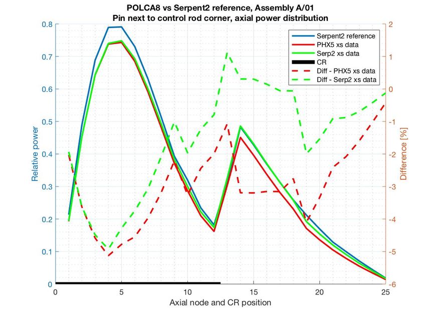
Mathilde Gaillard, MSc                                            Master Thesis Report

Abreviations
2D: two-dimensional
3D: three-dimensional
BA: Burnable Absorbers
BWR: Boiling Water Reactor
CBH: Control Blade History
CCCP: Current Coupling Collision Probability
CC: Current Coupling
CP: Collision Probability
CR Control Rods
CRAM: Chebyshev Rational Approximation Method
LWR: Light Water Reactor
MC: Monte Carlo
PHX5 xs data: PHOENIX5 cross section data
Serp xs data: Serpent2 cross section data

Westinghouse Eletric Sweden AB, Västerås, Sweden, February 2021                     v
Contents

Aknowledgement                                                                                                                                                     ii

Abstract                                                                                                                                                          iii

Sammanfattning                                                                                                                                                    iv

Abreviations                                                                                                                                                       v

List of Figures                                                                                                                                                    x

List of Tables                                                                                                                                                    xi

Presentation of the company                                                                                                                                       xii

1   Introduction                                                                                                                                                   1
    1.1 Nodal core analysis methodology . . . . . . . . . . . . . . . . . . . . . . . . . . . . . . . . .                                                          1
    1.2 Mission for the project . . . . . . . . . . . . . . . . . . . . . . . . . . . . . . . . . . . . . .                                                        3

2   Codes in use and cross-section generation                                                                                                                      4
    2.1 The stochastic Monte Carlo transport code Serpent2            .   .   .   .   .   .   .   .   .   .   .   .   .   .   .   .   .   .   .   .   .   .   .    4
    2.2 The deterministic transport code PHOENIX5 . . .               .   .   .   .   .   .   .   .   .   .   .   .   .   .   .   .   .   .   .   .   .   .   .    5
    2.3 The nodal core simulator POLCA8 . . . . . . . . .             .   .   .   .   .   .   .   .   .   .   .   .   .   .   .   .   .   .   .   .   .   .   .    6
        2.3.1 Cross-section model . . . . . . . . . . . .             .   .   .   .   .   .   .   .   .   .   .   .   .   .   .   .   .   .   .   .   .   .   .    6
        2.3.2 Pin power reconstruction methodology . .                .   .   .   .   .   .   .   .   .   .   .   .   .   .   .   .   .   .   .   .   .   .   .    8
    2.4 Cross-section generation methodology . . . . . . .            .   .   .   .   .   .   .   .   .   .   .   .   .   .   .   .   .   .   .   .   .   .   .    9

3   Specification of benchmark problems                                                                                                                           11
    3.1 Description of the configurations . . . . . . . .     .   .   .   .   .   .   .   .   .   .   .   .   .   .   .   .   .   .   .   .   .   .   .   .   .   11
         3.1.1 Benchmark configuration . . . . . . . .        .   .   .   .   .   .   .   .   .   .   .   .   .   .   .   .   .   .   .   .   .   .   .   .   .   11
         3.1.2 The Control Blade History (CBH) effect         .   .   .   .   .   .   .   .   .   .   .   .   .   .   .   .   .   .   .   .   .   .   .   .   .   13
    3.2 Setting up the reference solution in Serpent2 . .     .   .   .   .   .   .   .   .   .   .   .   .   .   .   .   .   .   .   .   .   .   .   .   .   .   14
         3.2.1 Bias in the multiplication factor . . . .      .   .   .   .   .   .   .   .   .   .   .   .   .   .   .   .   .   .   .   .   .   .   .   .   .   14
         3.2.2 Convergence of the fission source . . .        .   .   .   .   .   .   .   .   .   .   .   .   .   .   .   .   .   .   .   .   .   .   .   .   .   15
         3.2.3 Void Profile . . . . . . . . . . . . . . .     .   .   .   .   .   .   .   .   .   .   .   .   .   .   .   .   .   .   .   .   .   .   .   .   .   17
    3.3 Quantities of interest and statistics . . . . . . .   .   .   .   .   .   .   .   .   .   .   .   .   .   .   .   .   .   .   .   .   .   .   .   .   .   17
    3.4 Normalization of the results . . . . . . . . . . .    .   .   .   .   .   .   .   .   .   .   .   .   .   .   .   .   .   .   .   .   .   .   .   .   .   17

                                                       vi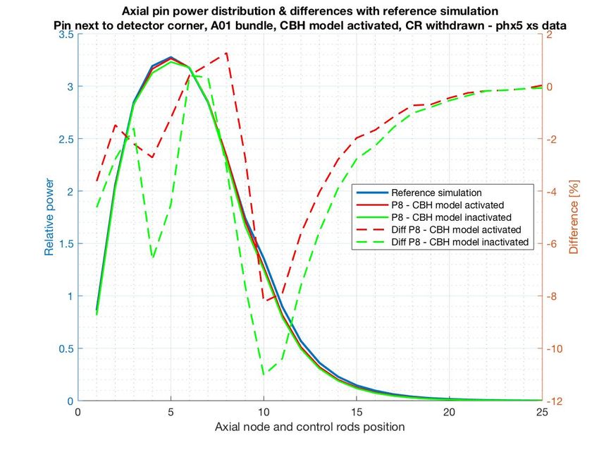
Mathilde Gaillard, MSc                                                                                                        Master Thesis Report

4   Results                                                                                                                                                       19
    4.1 Analysis at the fresh core conditions . . . . .   .   .   .   .   .   .   .   .   .   .   .   .   .   .   .   .   .   .   .   .   .   .   .   .   .   .   19
         4.1.1 Core multiplication factor predictions     .   .   .   .   .   .   .   .   .   .   .   .   .   .   .   .   .   .   .   .   .   .   .   .   .   .   19
         4.1.2 Nodal power distributions . . . . . .      .   .   .   .   .   .   .   .   .   .   .   .   .   .   .   .   .   .   .   .   .   .   .   .   .   .   20
         4.1.3 Pin power distributions . . . . . . . .    .   .   .   .   .   .   .   .   .   .   .   .   .   .   .   .   .   .   .   .   .   .   .   .   .   .   21
    4.2 Analysis of the depleted core conditions . . .    .   .   .   .   .   .   .   .   .   .   .   .   .   .   .   .   .   .   .   .   .   .   .   .   .   .   23
         4.2.1 Core multiplication factor predictions     .   .   .   .   .   .   .   .   .   .   .   .   .   .   .   .   .   .   .   .   .   .   .   .   .   .   24
         4.2.2 Nodal power distributions . . . . . .      .   .   .   .   .   .   .   .   .   .   .   .   .   .   .   .   .   .   .   .   .   .   .   .   .   .   26
         4.2.3 Pin power distributions . . . . . . . .    .   .   .   .   .   .   .   .   .   .   .   .   .   .   .   .   .   .   .   .   .   .   .   .   .   .   30

5   Conclusions                                                                                                                                                   38

Bibliography                                                                                                                                                      40

Appendix                                                                                                                                                          41

A Development of results analysis tools                                                                                                                           42
  A.1 Resuts format . . . . . . . . . . . . . . . . . . . . . . . . . . . . . . . . . . . . . . . . . . .                                                         42
  A.2 The Matlab analysis tool . . . . . . . . . . . . . . . . . . . . . . . . . . . . . . . . . . . . .                                                          43

B Gantt chart and diagram of tasks performed                                                                                                                      45

C Results at fresh core conditions                                                                                                                                47
  C.1 Axial pin power distribution . . . . . . . . . . . . .              .   .   .   .   .   .   .   .   .   .   .   .   .   .   .   .   .   .   .   .   .   .   47
  C.2 Radial pin power distribution . . . . . . . . . . . . .             .   .   .   .   .   .   .   .   .   .   .   .   .   .   .   .   .   .   .   .   .   .   48
       C.2.1 Axial node 5, PHOENIX5 cross section data                    .   .   .   .   .   .   .   .   .   .   .   .   .   .   .   .   .   .   .   .   .   .   49
       C.2.2 Axial node 5, Serpent2 cross section data . .                .   .   .   .   .   .   .   .   .   .   .   .   .   .   .   .   .   .   .   .   .   .   50
       C.2.3 Axial node 12, PHOENIX5 cross section data                   .   .   .   .   .   .   .   .   .   .   .   .   .   .   .   .   .   .   .   .   .   .   51
       C.2.4 Axial node 12, Serpent2 cross section data .                 .   .   .   .   .   .   .   .   .   .   .   .   .   .   .   .   .   .   .   .   .   .   52
       C.2.5 Axial node 13, PHOENIX5 cross section data                   .   .   .   .   .   .   .   .   .   .   .   .   .   .   .   .   .   .   .   .   .   .   53
       C.2.6 Axial node 13, Serpent2 cross section data .                 .   .   .   .   .   .   .   .   .   .   .   .   .   .   .   .   .   .   .   .   .   .   54
       C.2.7 Axial node 14, PHOENIX5 cross section data                   .   .   .   .   .   .   .   .   .   .   .   .   .   .   .   .   .   .   .   .   .   .   55
       C.2.8 Axial node 14, Serpent2 cross section data .                 .   .   .   .   .   .   .   .   .   .   .   .   .   .   .   .   .   .   .   .   .   .   56

D Results with PHOENIX5 cross section data, depleted core conditions                                                                                              57
  D.1 Axial pin power distribution . . . . . . . . . . . . . . . . . . . . .                              .   .   .   .   .   .   .   .   .   .   .   .   .   .   57
       D.1.1 Control rods corner . . . . . . . . . . . . . . . . . . . . . .                              .   .   .   .   .   .   .   .   .   .   .   .   .   .   57
       D.1.2 Detector corner . . . . . . . . . . . . . . . . . . . . . . . .                              .   .   .   .   .   .   .   .   .   .   .   .   .   .   58
  D.2 Radial pin power distribution . . . . . . . . . . . . . . . . . . . . .                             .   .   .   .   .   .   .   .   .   .   .   .   .   .   59
       D.2.1 Axial node 13, control rods half inserted . . . . . . . . . . .                              .   .   .   .   .   .   .   .   .   .   .   .   .   .   60
       D.2.2 Axial node 5, CBH model activated . . . . . . . . . . . . .                                  .   .   .   .   .   .   .   .   .   .   .   .   .   .   61
       D.2.3 Axial node 5, CBH model inactivated . . . . . . . . . . . .                                  .   .   .   .   .   .   .   .   .   .   .   .   .   .   62
       D.2.4 Axial node 12, CBH model activated . . . . . . . . . . . .                                   .   .   .   .   .   .   .   .   .   .   .   .   .   .   63
       D.2.5 Axial node 12, CBH model inactivated . . . . . . . . . . .                                   .   .   .   .   .   .   .   .   .   .   .   .   .   .   64
       D.2.6 Axial node 14, CBH model activated . . . . . . . . . . . .                                   .   .   .   .   .   .   .   .   .   .   .   .   .   .   65
       D.2.7 Axial node 14, CBH model inactivated . . . . . . . . . . .                                   .   .   .   .   .   .   .   .   .   .   .   .   .   .   66

Westinghouse Eletric Sweden AB, Västerås, Sweden, February 2021                                                                                                   vii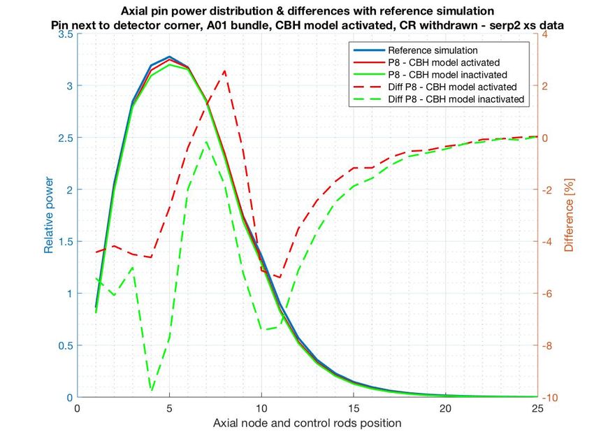
Mathilde Gaillard, MSc                                                                                  Master Thesis Report

E Results with Serpent2 cross section data, depleted core conditions                                                                         67
  E.1 Axial pin power distribution . . . . . . . . . . . . . . . . . . .    .   .   .   .   .   .   .   .   .   .   .   .   .   .   .   .    67
       E.1.1 Control rods corner . . . . . . . . . . . . . . . . . . . .    .   .   .   .   .   .   .   .   .   .   .   .   .   .   .   .    67
       E.1.2 Detector corner . . . . . . . . . . . . . . . . . . . . . .    .   .   .   .   .   .   .   .   .   .   .   .   .   .   .   .    68
  E.2 Radial pin power distribution . . . . . . . . . . . . . . . . . . .   .   .   .   .   .   .   .   .   .   .   .   .   .   .   .   .    69
       E.2.1 Axial node 13, control rods half-inserted . . . . . . . .      .   .   .   .   .   .   .   .   .   .   .   .   .   .   .   .    70
       E.2.2 Axial node 5, CBH model activated . . . . . . . . . . .        .   .   .   .   .   .   .   .   .   .   .   .   .   .   .   .    71
       E.2.3 Axial node 5, CBH model inactivated . . . . . . . . . .        .   .   .   .   .   .   .   .   .   .   .   .   .   .   .   .    72
       E.2.4 Axial node 12, CBH model activated . . . . . . . . . .         .   .   .   .   .   .   .   .   .   .   .   .   .   .   .   .    73
       E.2.5 Axial node 12, CBH model inactivated . . . . . . . . .         .   .   .   .   .   .   .   .   .   .   .   .   .   .   .   .    74
       E.2.6 Axial node 14, CBH model activated . . . . . . . . . .         .   .   .   .   .   .   .   .   .   .   .   .   .   .   .   .    75
       E.2.7 Axial node 14, CBH model inactivated . . . . . . . . .         .   .   .   .   .   .   .   .   .   .   .   .   .   .   .   .    76

Westinghouse Eletric Sweden AB, Västerås, Sweden, February 2021                                                                             viii
List of Figures
1.1 Lattice cell used in this project . . . . . . . . . . . . . . . . . . . . . . . . . . . . . . . . . . 2
3.1 Fuel assemblies at the bottom of the core . . . . . . . . . . . . . . . . . . . . . . . . . . . . . 12
3.2 Axial subdivision of the core . . . . . . . . . . . . . . . . . . . . . . . . . . . . . . . . . . . 12
3.3 The imposed axial coolant density profile in POLCA8 and Serpent2 calculations . . . . . . . . 13
3.4 Stabilisation of the Shannon entropy as function of the number of inactive cycles . . . . . . . 15
3.5 Convergence of the eigenvalue as function of the number of inactive cycles . . . . . . . . . . 16
4.1 Comparison between PHX5/POLCA8 and Serp2/POLCA8 against 3D Serpent2 reference
simulation for the nodal power in the bundle A/01, CBH model inactivated . . . . . . . . . . . 21
4.2 Differences in the axial pin power distribution between POLCA8 simulations and the reference
simulation inside bundle A/01, pin next to CR corner . . . . . . . . . . . . . . . . . . . . . . 22
4.3 Differences in the axial pin power distribution between POLCA8 simulations and the reference
simulation inside bundle A/01, pin next to detector corner . . . . . . . . . . . . . . . . . . . . 22
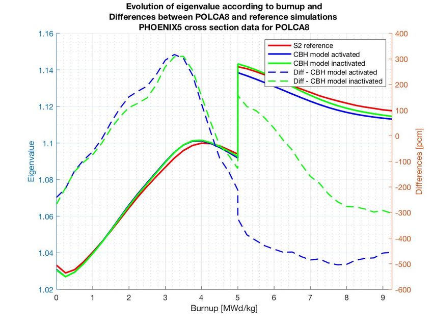
4.4 Eigenvalue evolution and differences between PHOENIX5/POLCA8 and Serpent2 reference
simulations . . . . . . . . . . . . . . . . . . . . . . . . . . . . . . . . . . . . . . . . . . . . 24
4.5 Eigenvalue evolution and differences between Serpent2/POLCA8 and Serpent2 reference
simulations . . . . . . . . . . . . . . . . . . . . . . . . . . . . . . . . . . . . . . . . . . . . 25
4.6 Differences in the axial power distribution between PHOENIX5/POLCA8 and the Serpent2
reference simulations inside bundle A/01 during burnup with CBH model activated . . . . . . 27
4.7 Differences in the axial power distribution between PHOENIX5/POLCA8 and the Serpent2
reference simulations inside bundle A/01 during burnup with CBH model inactivated . . . . . 28
4.8 Differences in the axial power distribution between Serpent2/POLCA8 and the Serpent2
reference simulations inside bundle A/01 during burnup with CBH model activated . . . . . . 28
4.9 Differences in the axial power distribution between Serpent2/POLCA8 and the Serpent2
reference simulations inside bundle A/01 during burnup with CBH model inactivated . . . . . 29
4.10 PHOENIX5/POLCA8 axial power distributions at the withdrawal of the control rod . . . . . . 29
4.11 Serpent2/POLCA8 axial power distributions at the withdrawal of the control rod . . . . . . . . 30
4.12 Differences in the axial pin power distributions between POLCA8 and Serpent2 reference
simulations inside bundle A/01, the pin next to the control rod corner pin with CR inserted,
PHX5 xs data . . . . . . . . . . . . . . . . . . . . . . . . . . . . . . . . . . . . . . . . . . . 31
4.13 Differences in the axial pin power distributions between POLCA8 and Serpent2 reference
simulations inside bundle A/01, the pin next to the control rod corner pin with CR withdrawn,
PHX5 xs data . . . . . . . . . . . . . . . . . . . . . . . . . . . . . . . . . . . . . . . . . . . 31
ixMathilde Gaillard, MSc Master Thesis Report
4.14 Differences in the axial pin power distributions between POLCA8 and Serpent2 reference
simulations inside bundle A/01, the pin next to the control rod corner pin with CR inserted,
Serp2 xs data . . . . . . . . . . . . . . . . . . . . . . . . . . . . . . . . . . . . . . . . . . . 32
4.15 Differences in the axial pin power distributions between POLCA8 and Serpent2 reference
simulations inside bundle A/01, the pin next to the control rod corner pin with CR withdrawn,
Serp2 xs data . . . . . . . . . . . . . . . . . . . . . . . . . . . . . . . . . . . . . . . . . . . 32
4.16 Differences in the axial pin power distributions between POLCA8 and Serpent2 reference
simulations inside bundle A/01, the pin next to the detector corner pin with CR inserted, PHX5
xs data . . . . . . . . . . . . . . . . . . . . . . . . . . . . . . . . . . . . . . . . . . . . . . . 33
4.17 Differences in the axial pin power distributions between POLCA8 and Serpent2 reference
simulations inside bundle A/01, the pin next to the detector corner pin with CR withdrawn,
PHX5 xs data . . . . . . . . . . . . . . . . . . . . . . . . . . . . . . . . . . . . . . . . . . . 33
4.18 Differences in the axial pin power distributions between POLCA8 and Serpent2 reference
simulations inside bundle A/01, the pin next to the detector corner pin with CR inserted, Serp2
xs data . . . . . . . . . . . . . . . . . . . . . . . . . . . . . . . . . . . . . . . . . . . . . . . 34
4.19 Differences in the axial pin power distributions between POLCA8 and Serpent2 reference
simulations inside bundle A/01, the pin next to the detector corner pin with CR withdrawn,
Serp2 xs data . . . . . . . . . . . . . . . . . . . . . . . . . . . . . . . . . . . . . . . . . . . 34
4.20 Differences in the radial pin power distribution between PHOENIX5/POLCA8 and Serpent2
reference simulations inside axial node 13 of bundle A/01 at the burnup point of CR withdrawal
(CRout) and with the CBH model activated . . . . . . . . . . . . . . . . . . . . . . . . . . . 35
4.21 Differences in the radial pin power distribution between PHOENIX5/POLCA8 and Serpent2
reference simulations inside axial node 13 of bundle A/01 at the burnup point of CR withdrawal
(CRout) and with the CBH model inactivated . . . . . . . . . . . . . . . . . . . . . . . . . . 36
4.22 Differences in the radial pin power distribution between Serpent2/POLCA8 and Serpent2
reference simulations inside axial node 13 of bundle A/01 at the burnup point of CR withdrawal
(CRout) and with the CBH model activated . . . . . . . . . . . . . . . . . . . . . . . . . . . 37
4.23 Differences in the radial pin power distribution between Serpent2/POLCA8 and Serpent2
reference simulations inside axial node 13 of bundle A/01 at the burnup point of CR withdrawal
(CRout) and with the CBH model activated . . . . . . . . . . . . . . . . . . . . . . . . . . . 37
Westinghouse Eletric Sweden AB, Västerås, Sweden, February 2021 xList of Tables
3.1 Bias in the eigenvalue for the evaluated 3D mini-core . . . . . . . . . . . . . . . . . . . . . . 15
4.1 Core eigenvalues . . . . . . . . . . . . . . . . . . . . . . . . . . . . . . . . . . . . . . . . . 20
4.2 Reactivity components . . . . . . . . . . . . . . . . . . . . . . . . . . . . . . . . . . . . . . 20
4.3 Summary of radial pin power distributions . . . . . . . . . . . . . . . . . . . . . . . . . . . . 23
4.4 Core eigenvalues at the withdrawal of the control rod . . . . . . . . . . . . . . . . . . . . . . 25
4.5 Reactivity components at the withdrawal of the control rod for PHOENIX5 cross section data . 26
4.6 Reactivity components at the withdrawal of the control rod for Serpent2 cross section data . . 26
4.7 Differences in the radial power distributions between POLCA8 simulations and the Serpent2
reference solution at the burnup point of the withdrawal of the control rod . . . . . . . . . . . 26
4.8 Summary of radial pin power errors at the control rod withdrawal point (PHX5 xs data) . . . . 35
4.9 Summary of radial pin power distributions at the withdrawal point. Serp2 xs data . . . . . . . 36
xiMathilde Gaillard, MSc Master Thesis Report
Presentation of the company
Westinghouse Electric Compagny LLC is an American nuclear power company created in 1999. It was
the former nuclear power division of the original Westinghouse Electric Corporation. Westinghouse Electric
Corporation was founded in 1886 and helped in developing electric infrastructure throughout the United States
thanks to the first industrial AC system for generating power. The company helped the US government’s military
program for nuclear energy applications by building the reactor on the world’s first nuclear submarine, and
was also instrumental in the development and commercialization of nuclear energy systems for electric power
generation. The world’s first pressurised water reactor (PWR) was designed and built by Westinghouse in
1957 in Shippingport, Pennsylvania, U.S. Nowadays, Westinghouse nuclear technologies are used in several
countries such as France, EDF is a long-time licensee of them, or Sweden with the Ringhals Nuclear Power Plant.
In Sweden, Westinghouse designed and built 12 nuclear power reactors between 1966 and 1985. As part
of the Swedish nuclear program, a nuclear fuel manufacturing plant was established in 1966 in Västerås.
Westinghouse bought it in 2000. This is one of the most modern nuclear fuel manufacturing plants in the world
with a capacity of 900 tonnes of uranium per year and a production of nuclear fuel, fuel components and control
rods. Within this manufacturing plant, an engineering service centre was developed to participate in the research,
development, production, testing and licensing of nuclear fuel. This engineering service centre also acts for the
maintenance of nuclear reactors such as boiling water reactor (BWR), PWR and water water energetic reactor
(VVER). Part of their work is to develop a new version of reactor simulator such as nodal core simulator.
Westinghouse Eletric Sweden AB, Västerås, Sweden, February 2021 xiiChapter 1
Introduction
1.1 Nodal core analysis methodology
Steady-state neutronics analysis of nuclear reactors relies on accurate computational methods for obtaining
the steady-state distribution of the free neutron population everywhere within the core. In Light Water Reactor
(LWR) analysis, computational methods for small-scale calculations are usually based on the neutron transport
theory, i.e. solving the Boltzmann transport equation. On the other hand, large-scale calculations are usually
based on a simplified version of the transport equation, namely, the diffusion equation [1]. Although the trans-
port equation is the most fundamental and accurate description of the spatial, energy and angular distribution
of neutrons, performing this type of calculation on an entire reactor core requires extensive computational
resources rendering such an approach rather impractical. Moreover, to analyse the behavior of a reactor core,
a lot of different simulations have to be considered, such as performing core follow calculations, evaluating
thermal margins during core surveillance or performing nuclear design calculations and fuel loading pattern
optimization. Consequently, a two-step methodology is adapted in nodal core analysis to predict the neutronic
behavior in the reactor core which comprises of two-dimensional (2D), multi-group lattice transport calculations
generating nodal cross section data to the nodal core simulator for various domains of the core, and subsequent
three-dimensional (3D) few-group nodal calculations considering the full reactor core.
The first step in this two-step nodal core analysis methodology is to perform calculations with a 2D neutron
transport code based on the more accurate neutron transport theory. These lattice calculations are not performed
on the whole core, but on a sub-region of the core called lattice cell with a fine spatial and energy mesh.
Figure 1.1 represents the lattice cell used for this project. A lattice cell typically represents a 1 cm thick
slice that contains a single fuel assembly plus half of the surrounding coolant gap in the radial direction. It
is accurately modeled in 2D geometry with materials characterized by fine-group cross-sections. Using the
reflective boundary condition, this unique lattice cell becomes an infinite large core, with only one type of fuel
assembly [2]. Thanks to generalized equivalence theory, preserving reaction rates and net leakages in an average
sense, the resulting neutron flux can be used for spatial homogenisation and condensation of cross-sections
(with respect to energy), as well as for computing discontinuity factors, pin power factors and other physics data
[3]. These homogenised nodal data will then be used in the second stage of the methodology by parameterizing
them as functions of important local state parameters and subsequently extracted by table interpolations or
polynomial fitting.
In the second step, a coarse spatial mesh is applied on the entire reactor core domain using diffusion
theory and pretabulated homogenized data obtained by lattice physics (previous step). The reactor core is
1Mathilde Gaillard, MSc Master Thesis Report
Figure 1.1: Lattice cell used in this project
subdivided into axial nodes of around 20 cm high with a base corresponding to the lattice cell i.e., one such
node corresponds to a single coarse-mesh point. In the nodal diffusion approach [4], the nodal balance equation,
derived from the 3D steady-state few group neutron diffusion equation, is solved within each node. Rather
than the conventional approach of finite differences to discrete the spatial variable, nodal methods use a high
order or analytical expansion of the intra-nodal flux shape to achieve a higher degree of accuracy for a given
node size. As a set of multi-dimensional equations is obtained, a transverse integration is often employed to get
a set of coupled one-dimensional equations. The resulting system is then solved on a 3D core composed by
homogeneous nodes characterized by the data previously generated.
To ensure that operating design and safety parameters, such as the minimum critical power ratio, stay below
the specified limits, the power generated in individual fuel rods is then estimated. If one wants to estimate
the fluxes in localized regions within the nodes, the nodal solution does not contain enough detail. For that, a
more detailed flux distribution is approximated from the nodal solution by superimposing the fine spatial mesh
transport solution upon the homogeneous intra-nodal flux solution, a procedure denoted flux reconstruction.
Using a two-step methodology instead of performing full core transport calculations directly on the problem
domain will introduce errors in the final results because of some additional assumptions inherent in this
procedure, such as:
• Application of reflective boundary conditions in the 2D lattice calculations thereby neglecting ant leakage
and spectrum interactions between fuel assemblies at the stage of generating cross section data.
• Assuming some representative core conditions during depletion neglecting the detailed local history that
is only known during the full core calculation.
These assumptions are addressed in the nodal core simulator by dedicated but approximative cross section and
pin power form function correction terms trying to compensate for these effects at the core level. Consequently,
assessing the capability of the nodal core simulator to handle and model these challenging real core conditions
using the two-step methodology is of crucial importance.
Westinghouse Eletric Sweden AB, Västerås, Sweden, February 2021 2Mathilde Gaillard, MSc Master Thesis Report
1.2 Mission for the project
This M.SC. project focuses on the second part of the nodal core analysis and its predictive capability. The
goal is to assess the accuracy of the PHOENIX5 [5] (the deterministic transport code of Westinghouse) and
POLCA8 [5] (the nodal core simulator of Westinghouse) code package in simulating challenging benchmark
problems anticipated from real core operation, this by comparing POLCA8 nodal and pin power distributions
against corresponding 3D full core Serpent2 [6] Monte Carlo transport results. For this purpose, a 3D boiling
water reactor (BWR) mini-core control blade history (CBH) benchmark has been constructed and evaluated in
this work to assess the accuracy of the dedicated cross section and pin power cross sections implemented in
POLCA8 to account for leakage effects and CBH.
In this evaluation, two sets of nodal cross section data (first step of the nodal core analysis) are used and
compared:
• Cross section data generated by the deterministic transport code PHOENIX5.
• Cross section data generated by the stochastic Monte Carlo code Serpent2.
By applying nodal cross section data generated by Serpent2 in the POLCA8 calculations, an unambiguous
comparison between POLCA8 and Serpent2 is obtained as the same transport solution methodology and cross
section library is used both for cross section generation and for obtaining the 3D reference solution.
This thesis is organized as follows. In Chapter 2, a description of the three codes used to carry out this
project is given, as well as an explanation of the methodology for generating multi-group cross-sections. In
Chapter 3, the specification of benchmark problems will be given through the description of the configuration,
how the reference simulation was set-up, and a presentation of the quantities of interest and statistics used will
be given too. Before the conclusion, the Chapter 4 will present the numerical results and their analysis.
Westinghouse Eletric Sweden AB, Västerås, Sweden, February 2021 3Chapter 2
Codes in use and cross-section generation
The purpose of this section is to provide a basic description of the methodology of the three codes used
for this project, which are the Serpent2 Monte Carlo stochastic transport code, the PHOENIX5 deterministic
transport code and the POLCA8 nodal core simulator. A description of how the cross-sections are generated
during lattice physics calculations will also be given, to facilitate the understanding of the work performed and
to highlight the challenges faced during this project.
2.1 The stochastic Monte Carlo transport code Serpent2
The Monte Carlo (MC) method is a way of solving complex problems such as neutron transport by a
stochastic approach using random numbers. This method is usually used on transport problems of high geomet-
rical complexity which are difficult to solve by a deterministic approach.
One of the major advantages of the MC method is its simplicity: the transport equation does not have to
be formulated to find the neutron flux inside the reactor as the a large batch of neutron histories is simulated
and the results are combined. It also allows the method to be able to simulate all types of reactor geometries
(either the simplest ones or the most complex ones). Another advantage of the MC method is its accuracy in
complex problem as the statistical errors decay as the square root of the batch size: the larger the sample, the
more accurate the results will be.
However, as previously mentioned, the MC method uses a stochastic approach, which will always induce
some statistical errors in the results. Therefore, even with a large batch size, the final result will still come with
some uncertainties. The other main disadvantage of the MC method is the computational resources needed to
resolve complex problems. The more complex the problem, the greater the resources required will be, especially
with a large neutron batch size, and especially for burnup simulations that requires many flux solutions.
The MC code used for this project is Serpent2. Serpent2 was first developed as a MC lattice transport code,
and is now developed as multipurpose MC reactor physics burnup calculation code capable to simulate various
complex systems, to generate group constants to fuel cycle analysis, or to calculate coupled multi-physics
problems [6].
Serpent2, as other MC codes, uses a three-dimensional constructive solid geometry model. This model is
built from elementary quadratic and derived surface types. Subsequently, these different surface types are used
4Mathilde Gaillard, MSc Master Thesis Report
to form two or three dimensional cells. It is also possible to create different levels inside the geometry by using
universes which will describe those levels.
Serpent2 uses a combination of two particle tracking methods:
• the ray-tracing based surface tracking method
• the rejection sampling based delta-tracking method
This last method allows neutron tracks to be continued over several material boundaries without calculating the
distances to the boundary surface, which leads to a speed-up in the transport simulation.
All neutron interaction data used in Serpent2 are coming from continuous-energy ACE format cross-section
libraries. Then, all cross-sections can be reconstructed by using a single unionized energy grid. With this
approach, it is possible to pre-calculate material-wise macroscopic cross-sections, and only one energy grid is
used to interpolate microscopic cross-sections between two tabulated values. Like that, the global calculation
time is significantly reduced. For the burnup simulations, all the data needed for isotopic transmutation (ra-
dioactive decay, energy-dependent fission yields and isomeric branching ratios) are read from ENDF format
data libraries. Serpent2 solves the Bateman depletion equations by using the CRAM (Chebyshev Rational
Approximation Method) matrix exponential method [7]. This method can handle the entire nuclide system
without any approximation for short-lived isotopes and cyclic processes, without step length limitation or numer-
ical accuracy problems. Although more advanced time integration schemes are available in Serpent2, such as
the Stochastic Implicit Euler method [8] [9] [10], a standard predictor-corrector scheme was utilized in this work.
To further speedup the calculations, Serpent2 employs a hybrid OpenMP/MPI parallelization scheme. In
addition, in order to fit large problems into the computer memory, domain decomposition is also available to
subdivide the problem into smaller pieces to be distributed over the used computing nodes.
Besides constituting the reference solution for the evaluated 3D mini-core problem, Serpent2 generates all
the nodal cross section data necessary for nodal diffusion calculations utilizing its built-in lattice physics branch
capabilities, such as the homogenized few-group macroscopic and microscopic cross-sections, the assembly
discontinuity factors and pin-wise power distributions for pin-power reconstruction. The cross section data
are all written in a Matlab m-file format that are further processed by Westinghouse in-house parser script
"serp2Latt" to convert these data to a format readable by the POLCA8 code package.
2.2 The deterministic transport code PHOENIX5
PHOENIX5 is an advanced lattice physics code developped by Westinghouse, based on the well-established
HELIOS lattice code with the main objective to create a reliable and robust tool for 2D neutron and gamma
transport calculations. Its main purpose is to accurately model light water reactor (LWR) fuel design, particularly
to cope with all the complexities of modern BWR reactor, and to generate nodal cross-section data for a 3D
simulator, POLCA8 as example. It can also be used in criticality analyses, control rod design, isotopic inventory
or make 2D reference calculations for others codes. PHOENIX5 mainly uses the ENDF/B-VII.1 cross-section
library with complements of JEFF-3, JENDL-4 and BROND-2.2 for gamma transport calculations [5].
Similar to HELIOS, PHOENIX5 uses the Current Coupling Collision Probability (CCCP) method to solve
the neutron and gamma transport equations. In this method, the system is divided into space elements, which are
Westinghouse Eletric Sweden AB, Västerås, Sweden, February 2021 5Mathilde Gaillard, MSc Master Thesis Report
further divided into flat-flux regions. They are internally treated by collision probabilities (CP). The coupling
of these space elements is done by the current coupling (CC) method using interface currents with angular
discretization on the hemisphere of the incoming directions [11] [12]. In orderto perform depletion calculations
and transmutation of isotopes, PHOENIX5 uses a standard predictor-corrector integration scheme employing
linearized nuclide chains.
As already explained in the Chapter 1, deterministic transport codes are used in the first step of nodal core
analysis to perform lattice physics calculations. The purpose of these calculations is to generate nodal cross
section data which will then be used by a nodal core simulator.
2.3 The nodal core simulator POLCA8
In nodal core analysis, after feeding generated nodal cross section data to the nodal core simulator of use,
3D reactor core simulations are conducted. The objective of this type of code is to simulate various conditions
foreseen for the design of a nuclear reactor core as well as perform core foloww calculations for real plant
operation. For example, the nodal core simulator of Westinghouse, POLCA (Power On-Line CAlculation), was
created in 1968 and has been used for many years to perform various BWR analyses such as core and fuel
design calculations, as well as core-tracking and in-core instrumentation evaluations.
As already explained in the Chapter 1, a nodal core simulator will solve the nodal diffusion equation on
a system subdivided into homogenized nodes, with each such node associated with the previously generated
nodal cross section data. Dedicated physics models are employed in the nodal core simulator to handle different
phenomena related to reactor physics, such as the cross section and pin power reconstruction being amongst the
most important. Consequently, both these models are discussed in more depth in the following.
2.3.1 Cross-section model
The cross-section model of POLCA8 is based on a combination of two types of terms:
• The ’base’ macroscopic cross-section, Σbase , obtained when a lattice code depletes the fuel at reference
conditions, i.e. depletion calculations where only the fuel exposure (burnup) is allowed to change while
all other state parameters are fixed to their so-called base values (nominal design values or typical average
values). In this regard, the coolant density and its history constitute important exceptions to the above
base condition and are included in the set of dependencies base cross sections posses.
• Deviation terms composed of instantaneous effects, depletion history effects and spatial homogenization
effects on cross sections.
The cross section model is mathematically expressed as:
Westinghouse Eletric Sweden AB, Västerås, Sweden, February 2021 6Mathilde Gaillard, MSc Master Thesis Report
Σ = Σbase (E, ρh , ρ) + δSG ∆ΣSG (E, ρh , ρ) + δCR ∆ΣCR (E, ρh , ρ, β )
+ δDT ∆ΣDT (E, ρh , ρ)
h i
+ cB (E, ρh , ρ) CB −CBbase
h i
base
+ cXe (E, ρh , ρ) NXe − NXe
hp q i
+ dDop (E, ρh , ρ) T f − T fbase
h i
+ cTm (E, ρh , ρ) Tm − Tmbase
h i
+ ∑ σi (E, ρh , ρ, wh , δCR , ...) Ni − Nibase (E, ρh , wCBH )
i
+ wCBH (1 − δCR ) ∆ΣCBH,out (E, ρh , ρ) + δCR ∆ΣCBH,in (E, ρh , ρ)
+ ∆Σspat + ∆Σleak + ∆Σhet,byp
(2.1)
During reconstruction, cross-sections are evaluated at a detailed axial sub-node level with a dependencies
on various state parameters, such as the burnup (expressed here as E, in MWd/kg), the coolant density history
(ρh in kg/m3 ) or the instantaneous coolant density (ρ in kg/m3 ). To convert the sub-node cross-section into the
corresponding nodal mesh used by the flux solver, axial homogenization is performed [13].
Some terms, such as the corrections for control rods and spacer grids (∆ΣCR and ∆ΣSG ), the off-base fuel
Doppler temperature (dDop .∆T f ), the xenon concentration (cXe .∆NXe ) and the soluble boron concentration
(cB .∆CB ) are generated by PHOENIX5 lattice physics calculations (first step of the nodal core analysis method-
ology). However, as PHOENIX5 (or Serpent2) lattice physics calculations are performed for an infinite fuel
lattice, certain assumptions are made during these lattice calculations, such as the absence of leakage. Therefore,
correction terms are estimated and computed by POLCA8 itself to account for neutron leakage effects (∆Σleak ),
as well as for intra-nodal depletion effects (∆Σspat ) [13].
During a burnup simulation, the control rods also experience a depletion of their own active absorber
material. This will have an impact on the cross-sections, as well and POLCA8 takes this into account in the
cross-section model. The depletion state of the control blade is quantified with the control blade depletion
fraction, β , include in the set of dependencies of the correction term for the control rods. Although cross-sections
are dependent on the coolant density history, some residual history effects are included by simulating real life
operation. Therefore, an isotropic correction term based on explicit microscopic depletion, ∑i σi ∆Ni , have been
add to the model [13].
The very challenging CBH effect, the main target of analysis of this study, is also handled with dedicated
correction terms. During the lattice physics calculations, the two extreme conditions of the CBH effect, when
the control rods are fully inserted during fuel depletion, ∆ΣCBH,in , and when they are fully withdrawn during
fuel depletion, ∆ΣCBH,out , are computed. POLCA8 then performs an interpolation between these two extreme
states to obtain the cross-section correction required for a certain control blade history condition [13]. Note
that by deactivating the CBH model in POLCA8, one is fully relying on that intra-nodal cross section model
corrections will capture the CBH effect, an assumption that has proven to be rather poor one.
Finally, to cope with certain transient conditions in the core, a term with an explicit dependence on the
moderator temperature is present, cTm .∆Tm , as well as a correction term to account for bypass water density and
Westinghouse Eletric Sweden AB, Västerås, Sweden, February 2021 7Mathilde Gaillard, MSc Master Thesis Report
soluble boron heterogeneities ∆Σhet,byp . If detectors are present inside the core, their geometrical effects on the
cross-sections are also taken into account thanks to one special correction term, ∆ΣDT [13].
2.3.2 Pin power reconstruction methodology
In POLCA8, pin powers are calculated inside a materially homogeneous sub-node s, and are expressed as
volumetric power densities. A sub-node is obtained after the breaking down of a node, if this node presents
material heterogeneities in the axial direction due to the presence of burnable absorbers (BA)/enrichment
zoning, spacer grids or control rod for examples. The calculation of pin powers is based on a combination of
lattice code physics data and nodal core simulator results. The detailed relative power density is mathematically
expressed as:
2
p (x, y, z) = cnorm ∑ Sgrad (x, y) Sax (z) Pghom (x, y, z) (2.2)
g=1
The summation is over two energy groups and the basic assumption that the radial and axial heterogeneous
dependencies, represented by the shape function, are separable is made. The radial fine structure shape function,
Sgrad (x, y), is carried over the lattice code evaluation and is given for the given sub-node (one value per pin cell
and group). This transport solution accounts for the heterogeneous pin nature of the assembly and the CBH
effect. The axial fine structure shape function, Sax (z), accounts for the node the axial heterogeneities like spacer
grids, control rod tips, and enrichment/BA discontinuities. It is energy group independent, and the calculations
of it take place in the core itself. The coefficient cnorm is the normalisation factor, determined such that p (x, y, z)
averages Psub , the average relative power density for the given sub-node. The quantity Psub is known from the
axial homogeneization calculation. [14].
The last term of Equation 2.2, Pghom (x, y, z), is known as the homogeneous relative power density distribution
per energy group inside a full node and is obtained by solving the two-group diffusion equation with realistic
boundary conditions and with slowly varying (close to uniform) cross section. It accounts for global, smooth
power tilts caused by an uneven leakage of neutrons from neighbouring nodes and by the fact that the assembly
is depleted spatially differently in real life compared to the lattice calculations feeding the nodal core simulator
with cross section data. It can be mathematically expressed by the following equation:
κΣnode
f ,g Φg
node (x, y, z)
Vn
Pghom (x, y, z) = (2.3)
Qrel πV Vnf
where κΣnode node (x, y, z) is the smooth flux solution (i.e., plane
f ,g is the intra-nodal cross section profile, Φg
wave expansion in each energy group), Qrel is the relative core thermal power (W ), πv is the volumetric core
power density (W.m−3 ), Vn is the full node volume (m3 ) and Vnf is the node so-called "fissile" volume, i.e. only
multiplying axial segments of the node (m3 ) [14].
In Serpent2, one can access both nodal power distributions and pin power distributions inside the considered
system through the use of different options such as the cpd card or by a mesh detector. All these power
distributions are expressed in watt [6]. However, although data of same resolution can be accessed in POLCA8,
powers are specified in terms of relative values with regard to volumetric power densities. Consequently, and
before making comparisons between simulations, it is necessary to express results using the same unit. Since
the results of Serpent2 are expressed in watt, the choice was made to convert all powers computed by POLCA8
to the unit of watt.
Westinghouse Eletric Sweden AB, Västerås, Sweden, February 2021 8Mathilde Gaillard, MSc Master Thesis Report
In terms of nodal powers as predicted by POLCA8, one way to obtain the absolute nodal power in watt for
node n is given by Equation 2.4.
abs rel
Pn [W ] = Pn × Qrel × πv ×Vn
N (2.4)
1 ∑ Prel = 1.0
n
N n=1
where Pnrel is the relative nodal power density from POLCA8.
The method for converting pin powers is the same as that for nodal powers, with the exception of one term.
It is given by Equation 2.5 for pin i in node n.
1
abs rel
pi,n [W ] = pi,n × Q rel × π v ×Vn ×
Nf
N (2.5)
1 f rel rel
∑ pi,n = Pn
N f i=1
where prel
i,n is the raw data from POLCA8, and N f is the number of fuel pins inside the node n.
It is important to mention that Equation 2.4 and Equation 2.5 and their normalisation are only valid if all
nodes within the core have the same volume [14].
2.4 Cross-section generation methodology
As earlier described, the cross sections used during nodal simulations must be generated before starting
the calculations. They are generated by performing 2D lattice physics calculations employing a transport code,
i.e., in this project by using the deterministic transport code PHOENIX5 and the stochastic MC transport code
Serpent2.
For these lattice calculations, reflective boundary conditions are applied because it is assumed that the fuel
assembly properties depend mainly on the heterogeneous nature of the assembly itself and less on its location in
the reactor core. As several fuel assembly types are used within the core geometry, this set of calculations must
be applied for each of them. Indeed, each set of 2D lattice physics calculations represents a axial fuel assembly
segment type defined by its lattice and nuclear design (i.e. geometry, enrichment, BA loading, etc.) [15].
For each such fuel assembly segment type, a series of independent lattice depletion calculations have to
be carried out for given depletion histories, i.e., in this case for given void histories (or active coolant density
histories), combined with a large number of momentaneous branch calculations representing perturbations to
the conditions prevailing during depletion. Only the burnup is allowed to change during these lattice depletion
calculations, with all the other state parameters fixed at their base-values (i.e. nominal design values or typical
average values). In contrast, the branch calculations are taking into account momentaneous changes in the
operating conditions, such as the coolant density, the control rod insertion status, the xenon concentration and
the soluble boron concentration. These branches can be applied at different burnup steps chosen by the user.
They are normally performed independently for each state parameter, but a combination of different parameters
can also be done. For example, the momentaneous active coolant density is always varied simultaneously with
each one or a combination of the other state parameters. Furthermore, the depletion history cases should cover
the range of the expected values of the relevant history parameter, so that any extrapolation can be avoided
when reconstructing the cross section for each node in the core [15].
Westinghouse Eletric Sweden AB, Västerås, Sweden, February 2021 9Mathilde Gaillard, MSc Master Thesis Report
The base conditions defined for each coolant density history are described by the following state parameter
setup:
• Hot full power internal and external bypass moderator density corresponding to a saturated temperature
at nominal core pressure with no boiling in these bypasses.
• Hot full power active coolant density corresponding to a selected void condition (including zero void).
This also defines the coolant density history for the selected void content.
• Hot full power nominal power density.
• Hot full power nominal fuel temperature.
• No control rods present.
• No spacer grids present.
• No detector presents.
• Reference soluble boron concentration of 0 ppm.
• Equilibrium xenon at nominal power density.
The Control Blade History (CBH) having such a strong impact on the reactivity and the assembly-internal
power distribution, requires a speacial treatment. Consequently, dedicated CBH lattice calculations are per-
formed to generate CBH corrections to the base values of cross sections, discontinuity factors and pin power
form functions. These CBH correction tables are then tabulated as function of the momentaneous coolant
density, coolant density history and fuel assembly exposure [15].
The CBH lattice calculations are performed as follows:
• Control rods always inserted (i.e. rodded) base depletion calculation for each coolant density history at
hot full power both voided and non-voided conditions.
• Rodded coolant density branch calculations from rodded base depletion cases for each momentaneous
coolant density condition.
• Control rods withdrawal branch calculations from rodded base depletion cases also for each momenta-
neous coolant density condition.
Finally, it is worthwhile to mention that these lattice calculations can be very time demanding when
considering such calculations based on Serpent2. Consequently, only a subset of all possible and supported
branch cases were performed in this work, including:
• Coolant density branches.
• Zero xenon branches.
• Control rod insertion branches.
• Zero xenon and control rod insertion branches
Also, for Serpent2 cross section data simulations, PHOENIX5-based CBH-tables were applied, as these lattice
calculations are not currently supported by the Serpent2/POLCA8 methodology.
Westinghouse Eletric Sweden AB, Västerås, Sweden, February 2021 10Chapter 3
Specification of benchmark problems
This chapter will discuss the specification and implementation of the benchmark problem considered in this
work. Besides, a complete description of the simulations carried out will be provided, as well as how some
important parameters, such as the number of neutrons per cycle or the number of inactive cycles, were chosen
before running the reference simulation. A short discussion about the most important physical implications of
the CBH effect will also be given including the definitions of the parameters of interest for this project.
3.1 Description of the configurations
3.1.1 Benchmark configuration
The configuration used in this benchmark is a 3D 2x2 mini core, with three different fuel lattices in the
axial direction. Each lattice has its enrichment of fissile materials and percentage of burnable poison. The
fuel assembly lattices are based on a SVEA-09 Optima3 model for the Olkiluoto nuclear power plant, unit 2,
residing in Finland but with some simplifications. Consequently, and to facilitate the Serpent2 calculations, the
following assumptions are made:
• Water diamond and water cross are replaced with water pins
• A regular fuel pin pitch is used to facilitate the calculation of pin power
A radial representation of the mini-core system at the bottom of the core is shown by the Figure 3.1. In this
geometrical representation, the cruciform control rod is situated in the northwest corner of the problem domain.
As previously said, each fuel assembly lattice type in the axial direction has its own material composition,
described here from the bottom to the top of the core:
• Lattice 217: 4.15 w/o 235 U, 8x6.00 & 2x3.00 w/o Gd2 O3
• Lattice 219: 4.19 w/o 235 U, 8x6.00 & 4x3.00 w/o Gd2 O3
• Lattice 221: 4.15 w/o 235 U, 8x6.00 & 4x3.00 w/o Gd2 O3
Lattice 217 has a fewer amount of burnable poisons rods compared to the other two lattices. Therefore it is
expected to get a higher power production in the bottom part of the core than in the upper part.
To follow the conventional apporoach of nodalization normally employed in nodal core analysis, and also to
facilitate data processing after simulations, the core is subdivided into 25 axial nodes, as presented in Figure 3.2,
11Mathilde Gaillard, MSc Master Thesis Report
Figure 3.1: Fuel assemblies at the bottom of the core
where the ++ present the position of the control rod inside the core. This is also the spatial mesh used axially by
the flux solver of POLCA8. This figure also demonstrates the axial composition of the core, designed by the
numbers 217, 219, and 221, and the nodes where the control rod is present when they are half-inserted into the
core.
Figure 3.2: Axial subdivision of the core
This mini-core is depleted up to 10 MWd/kg starting at fresh conditions, with steps of 0.250 MWd/kg. The
control rod is half inserted up to 5.000 MWd/kg, and then withdrawn from the core. To obtain data at the burnup
Westinghouse Eletric Sweden AB, Västerås, Sweden, February 2021 12Mathilde Gaillard, MSc Master Thesis Report
point of 5.000 MWd/kg for both the rodded and unrodded condition, a small step at 4.999 MWd/kg was added
of to the POLCA8 and Serpent2 simulations.
Neutrons are kept inside the core in the radial direction thanks to the reflective boundary conditions. How-
ever, due to vacuum boundary conditions applied at the top and bottom edge of the core, a strong neutron flux
gradient and leakage will be induced in the axial direction of the core.
Inside a BWR core, coolant steam will be created inside the core. This leads to the creation of a void profile
between the bottom and the top of the core, which manifests itself as a change in coolant density, as shown
in Figure 3.3. Therefore, and to resemble real operation conditions as close as possible, a fixed axial coolant
density profile was imposed over the core. Also, fixed values of the moderator temperature, 559 K, and the
fuel Doppler temperature, 900 K, were applied in this benchmark problem. The xenon was set to equilibrium
conditions.
Figure 3.3: The imposed axial coolant density profile in POLCA8 and Serpent2 calculations
In order to avoid any thermal-hydraulic feedback in the POLCA8 calculations (i.e., enabling the use of
the above-fixed values of relevant state parameters), the thermal-hydraulics calculations in POLCA8 were
deactivated. In this way, unambiguous comparisons of results between Serpent2 and POLCA8 can be established.
3.1.2 The Control Blade History (CBH) effect
Inside a BWR, the control rod is inserted into the inter-assembly gaps that are normally filled with water.
They are also often inserted during a long irradiation period. These two conditions combined lead to tilted
distributions of power or flux compared to the unrodded situation. Subsequent withdrawal of the control rod
after such a rodded irradiation period will in turn cause a strong power peaking in the neighborhood of the
control rod blades, an effect called the CBH effect.
Westinghouse Eletric Sweden AB, Västerås, Sweden, February 2021 13You can also read