Development of four-dimensional variational assimilation system based on the GRAPES-CUACE adjoint model (GRAPES-CUACE-4D-Var V1.0) and its ...
←
→
Page content transcription
If your browser does not render page correctly, please read the page content below
Geosci. Model Dev., 14, 337–350, 2021
https://doi.org/10.5194/gmd-14-337-2021
© Author(s) 2021. This work is distributed under
the Creative Commons Attribution 4.0 License.

Development of four-dimensional variational assimilation
system based on the GRAPES–CUACE adjoint model
(GRAPES–CUACE-4D-Var V1.0) and its
application in emission inversion
Chao Wang1,2 , Xingqin An1 , Qing Hou1 , Zhaobin Sun3 , Yanjun Li1 , and Jiangtao Li1
1 Institute of Atmospheric Composition and Environmental Meteorology, Chinese Academy of Meteorological Sciences,
Beijing 100081, China
2 Department of Atmospheric and Oceanic Sciences, Fudan University, Shanghai 200438, China
3 Institute of Urban Meteorology, China Meteorological Administration, Beijing 100089, China

Correspondence: Xingqin An (anxq@cma.gov.cn)

Received: 7 November 2019 – Discussion started: 3 February 2020
Revised: 21 November 2020 – Accepted: 2 December 2020 – Published: 22 January 2021

Abstract. In this study, a four-dimensional variational (4D-    have greatly reduced from 2007 to 2016. In the future, fur-
Var) data assimilation system was developed based on            ther studies on improving the performance of the GRAPES–
the GRAPES–CUACE (Global/Regional Assimilation and              CUACE-4D-Var assimilation system are still needed and are
PrEdiction System – CMA Unified Atmospheric Chem-               important for air pollution research in China.
istry Environmental Forecasting System) atmospheric chem-
istry model, GRAPES–CUACE adjoint model and L-BFGS-
B (extended limited-memory Broyden–Fletcher–Goldfarb–
Shanno) algorithm (GRAPES–CUACE-4D-Var) and was ap-             1   Introduction
plied to optimize black carbon (BC) daily emissions in
northern China on 4 July 2016, when a pollution event oc-       Three-dimensional (3-D) atmospheric chemical transport
curred in Beijing. The results show that the newly con-         models (CTMs) are important tools for air quality research,
structed GRAPES–CUACE-4D-Var assimilation system is             which are used not only for predicting spatial and temporal
feasible and can be applied to perform BC emission inver-       distributions of air pollutants but also for providing sensi-
sion in northern China. The BC concentrations simulated         tivities of air pollutant concentrations with respect to various
with optimized emissions show improved agreement with           parameters (Hakami et al., 2007). Among several methods of
the observations over northern China with lower root-mean-      sensitivity analysis, the adjoint method is known to be an effi-
square errors and higher correlation coefficients. The model    cient means of calculating the sensitivities of a cost function
biases are reduced by 20 %–46 %. The validation with ob-        with respect to a large number of input parameters (Sandu
servations that were not utilized in the assimilation shows     et al., 2005; Hakami et al., 2007; Henze et al., 2007; Zhai
that assimilation makes notable improvements, with values       et al., 2018). The sensitivity information provided by the ad-
of the model biases reduced by 1 %–36 %. Compared with          joint approach can be applied to a variety of optimization
the prior BC emissions, which are based on statistical data     problems, such as formulating optimized pollution-control
of anthropogenic emissions for 2007, the optimized emis-        strategies, inverse modelling and variational data assimila-
sions are considerably reduced. Especially for Beijing, Tian-   tion (Liu, 2005; Hakami et al., 2007).
jin, Hebei, Shandong, Shanxi and Henan, the ratios of the op-      Four-dimensional variational (4D-Var) data assimilation,
timized emissions to prior emissions are 0.4–0.8, indicating    which is an important application of adjoint models, pro-
that the BC emissions in these highly industrialized regions    vides insight into various model inputs, such as initial condi-

Published by Copernicus Publications on behalf of the European Geosciences Union.
338                                   C. Wang et al.: Development of GRAPES–CUACE-4D-Var V1.0 and its application

tions and emissions (Liu, 2005; Yumimoto and Uno, 2006).         tainty will affect the accuracy of air pollution simulation,
In the past decades, many scholars have successively devel-      which in turn will affect the accuracy of pollution-control
oped adjoint models of various 3-D CTMs and the 4D-Var           measures based on the model results (Huang et al., 2018).
data assimilation systems to optimize model parameters. El-      In order to improve the accuracy of atmospheric chemistry
bern and Schmidt (1999, 2001), Elbern et al. (2000, 2007)        simulation and the feasibility of the pollution-control strate-
constructed the adjoint of the EURAD CTM and performed           gies, the emission data obtained by the “bottom–up” method
inverse modelling of emissions and chemical data assimila-       needs to be optimized, which can be done through the atmo-
tion. Sandu et al. (2005) built the adjoint of the comprehen-    spheric chemical variational assimilation system, to reduce
sive chemical transport model STEM-III and conducted the         the impact of emission uncertainty.
data assimilation in a twin-experiment framework as well            GRAPES–CUACE is an atmospheric chemistry model
as the assimilation of a real data set, with the control vari-   system developed by the Chinese Academy of Meteoro-
ables being O3 or NO2 . Hakami et al. (2005) applied the ad-     logical Sciences (CAMS) (Gong and Zhang, 2008; Zhou
joint model of the STEM-2k1 model for assimilating black         et al., 2008, 2012; Wang et al., 2010, 2015). GRAPES
carbon (BC) concentrations and the recovery of its emis-         (Global/Regional Assimilation and PrEdiction System) is a
sions. Liu (2005) and Huang et al. (2018) developed the ad-      numerical weather prediction system built by China Mete-
joint of the CAMx model and further expanded it into an          orological Administration (CMA), and it can be used as a
air quality forecasting and pollution-control decision sup-      global model (GRAPES-GFS) or as a regional mesoscale
port system. Müller and Stavrakou (2005) constructed an in-      model (GRAPES-Meso) (Chen et al., 2008; Zhang and Shen,
verse modelling framework based on the adjoint of the global     2008). CUACE (CMA Unified Atmospheric Chemistry En-
model IMAGES and used it to optimize the global annual           vironmental Forecasting System) is a unified atmospheric
CO and NOx emissions for the year 1997. More recently, the       chemistry model constructed by CAMS to study both air
CMAQ (Community Multiscale Air Quality Modeling Sys-             quality forecasting and climate change (Gong and Zhang,
tem) team (Hakami et al., 2007) built the adjoint of CMAQ        2008; Zhou et al., 2008, 2012). Using the meteorological
model and its 4D-Var assimilation scheme, which were used        fields provided by GRAPES-Meso, the GRAPES–CUACE
to optimize NOx emissions (Kurokawa et al., 2009; Resler         model has realized the online coupling of meteorology and
et al., 2010) and ozone initial state (Park et al., 2016). The   chemistry (Gong and Zhang, 2008; Zhou et al., 2008, 2012;
adjoints of the GEOS-Chem model and its 4D-Var assimi-           Wang et al., 2010, 2015). The GRAPES–CUACE model not
lation system first developed by Henze et al. (2007, 2009)       only plays an important role in the scientific research on air
have been applied in a number of studies to improve aerosol      pollution in China (Gong and Zhang, 2008; Zhou et al., 2008,
(Wang et al., 2012; Mao et al., 2015; Jeong and Park, 2018),     2012; Wang et al., 2010, 2015) but has also been officially in
CO (Jiang et al., 2015) and NMVOC (non-methane volatile          operation since 2014 at the National Meteorological Center
organic compound) (Cao et al., 2018) emission estimates.         of CMA for providing guidance for air quality forecasting
Zhang et al. (2016) applied the 4D-Var assimilation sys-         over China (Ke, 2019).
tem using the adjoint model of GEOS-Chem with the fine              Recently, An et al. (2016) constructed the aerosol adjoint
1/4◦ × 5/16◦ horizontal resolution to optimize daily aerosol     module of the GRAPES–CUACE model, which was subse-
primary and precursor emissions over northern China. This        quently applied in tracking influential BC and PM2.5 source
research has laid good foundations for developing adjoint        areas in northern China (Zhai et al., 2018; Wang et al., 2018a,
models of CTMs and optimizing model parameters. How-             2018b, 2019). However, these applications of GRAPES–
ever, only a few of these adjoint models and their 4D-Var        CUACE aerosol adjoint model are still limited to sensitiv-
assimilation systems have been widely applied to regional        ity analysis, and the sensitivity information is not fully used
air pollution in China. The development and applications of      to solve various optimization problems mentioned above. At
adjoint models of 3-D CTMs and their 4D-Var data assimila-       the same time, considering the current severe pollution situ-
tion systems are still limited in China. Further research and    ation in mega urban agglomerations in China, more accurate
more attention are required.                                     emission data are urgently required to formulate reasonable
   Nowadays, several mega urban agglomerations in China,         and effective pollution-control strategies. In this study, we
such as the Beijing–Tianjin–Hebei region, the Yangtze River      developed a new 4D-Var data assimilation system on the ba-
Delta region and the Fenwei Plain, are still suffering from      sis of the GRAPES–CUACE adjoint model, which was ap-
severe air pollution (Zhang et al., 2019; Xiang et al., 2020;    plied for assimilating surface BC concentrations and opti-
Haque et al., 2020; Zhao et al., 2020). Previous studies have    mizing its daily emissions in northern China on 4 July 2016,
shown that emission-reduction strategies, which are mainly       when a pollution event occurred in Beijing. The following
based on the results of atmospheric chemistry simulations,       part is divided into four sections. Section 2 introduces the
play an important role in reducing pollutant concentrations      data and methods, Sect. 3 describes the GRAPES–CUACE-
and improving air quality (Zhang et al., 2016; Zhai et al.,      4D-Var assimilation system, Sect. 4 presents the results and
2016). The emission inventory represents important basic         discussions, and the conclusions are found in Sect. 5.
data for atmospheric chemistry simulation, and its uncer-

Geosci. Model Dev., 14, 337–350, 2021                                              https://doi.org/10.5194/gmd-14-337-2021
C. Wang et al.: Development of GRAPES–CUACE-4D-Var V1.0 and its application                                                 339

2     Methodology                                                 in the atmosphere are comprehensively considered in the
                                                                  CUACE model (Wang et al., 2015).
2.1     Forward model description                                    CUACE adopts CAM (Canadian Aerosol Module; Gong
                                                                  et al., 2003) and RADM II (the second-generation Re-
2.1.1    GRAPES-Meso                                              gional Acid Deposition Model; Stockwell et al., 1990) as
                                                                  its aerosol module and gaseous chemistry module, respec-
GRAPES-Meso is a real-time operational weather forecast-          tively. CAM involves six types of aerosols: sulfate (SF), ni-
ing model used by China Meteorological Administration             trate (NI), sea salt (SS), BC, organic carbon (OC) and soil
(Chen et al., 2008; Zhang and Shen, 2008). The GRAPES-            dust (SD), which are segregated into 12 size bins with di-
Meso model uses fully compressible non-hydrostatic equa-          ameter ranging from 0.01 to 40.96 µm according to the mul-
tions as its model core. The vertical coordinates adopt the       tiphase multicomponent aerosol particle size separation al-
height-based, terrain-following coordinates, and the hori-        gorithm (Gong et al., 2003; Zhou et al., 2008, 2012; Wang
zontal coordinates use the spherical coordinates of equal         et al., 2010, 2015). CAM also calculates the vertical diffu-
longitude–latitude grid points. The horizontal discretization     sion trend of aerosol particles by solving the vertical dif-
adopts an Arakawa-C staggered grid arrangement and a              fusion equation. The core of CAM is the aerosol physical
central finite-difference scheme with second-order accuracy,      and chemical processes, including hygroscopic growth, co-
while the vertical discretization adopts the vertically stag-     agulation, nucleation, condensation, dry deposition or sedi-
gered variable arrangement proposed by Charney-Phillips           mentation, below-cloud scavenging, and aerosol activation,
(Charney and Phillips, 1953). The time integration dis-           which is coherently integrated with the gaseous chemistry in
cretization uses a semi-implicit and semi-Lagrangian tem-         CUACE (Gong et al., 2003; Zhou et al., 2008, 2012; Wang
poral advection scheme. The large-scale transport processes       et al., 2010, 2015). The gas chemistry provides the produc-
(both horizontal and vertical) for all gases and aerosols in      tion rates of sulfate aerosols and secondary organic aerosols
GRAPES–CUACE are calculated by the dynamic framework              (SOAs) and meanwhile generates an oxidation background
of GRAPES-Meso, which implements the quasi-monotone               for aqueous-phase aerosol chemistry, in which sulfate trans-
semi-Lagrangian (QMSL) semi-implicit scheme on each grid          formation changes the distributions of SO2 in clouds (Zhou
(Wang et al., 2010). The physical processes principally in-       et al., 2012). Both nucleation and condensation are consid-
volve microphysical precipitation, cumulus convection, ra-        ered for sulfate aerosol formation depending on the atmo-
diative transfer, land surface and boundary layer processes.      spheric state after gaseous H2 SO4 formed from the oxidation
Each physical process incorporates several schemes and can        of sulfurous gases such as SO2 , H2 S and DMS (dimethyl
also be tailored by the user (Xu et al., 2008). The major phys-   sulfide) (Zhou et al., 2012). Secondary organic aerosols as
ical options that we selected include the WSM6 cloud mi-          generated from gaseous precursors are partitioned into dif-
crophysics scheme (Hong and Lim, 2006), the Betts–Miller–         ferent bins through condensation using the same approach
Janjic cumulus convection scheme (Betts and Miller, 1986;         as the gaseous H2 SO4 condensation to sulfate (Zhou et al.,
Janjić, 1994), the RRTM (Rapid Radiative Transfer Model;         2012). Given that the NIs and ammonium (AM) formed
Mlawer et al., 1997) long-wave radiation scheme, the short-       through the gaseous oxidation are unstable and prone to fur-
wave scheme based on Dudhia (1989), the Monin–Obukhov             ther decomposition back to their precursors, CUACE adopts
surface layer scheme (Monin and Obukhov, 1954), the MRF           ISORROPIA to calculate the thermodynamic equilibrium be-
(medium-range forecast) planetary boundary layer scheme           tween them and their gas precursors (West et al., 1998; Nenes
(Hong and Pan, 1996) and the Noah land surface scheme             et al., 1998a, b; Zhou et al., 2012). ISORROPIA contains
(Chen et al., 1996).                                              15 equilibrium reactions, and the main species include the
                                                                  gas phase (NH3 , HNO3 , HCL, H2 O), liquid phase (NH+       4,
2.1.2    CUACE                                                        +    +    −       −     2−       −    −
                                                                  Na , H , Cl , NO3 , SO4 , HSO4 , OH , H2 O) and solid
                                                                  phase ((NH4 )2 SO4 , NH4 HSO4 , (NH4 )3 H(SO4 )2 , NH4 NO3 ,
The atmospheric chemistry model CUACE mainly includes             NH4 Cl, NaCl, NaNO3 , NaHSO4 , Na2 SO4 ) (Nenes et al.,
three modules: the aerosol module (module_ae_cam), the            1998a).
gaseous chemistry module (module_gas_radm) and the ther-             The emissions used in this study are based on statisti-
modynamic equilibrium module (module_isopia) (Gong and            cal data of anthropogenic emissions reported from govern-
Zhang, 2008; Zhou et al., 2008, 2012; Wang et al., 2010,          ment agencies for 2007 (Cao et al., 2011). Emission source
2015). The interface program that connects CUACE and              types included residences, industry, power plants, transporta-
GRAPES-Meso is called aerosol_driver.F. This program              tion, biomass combustion, livestock and poultry breeding,
transmits the meteorological fields calculated in GRAPES-         fertilizer use, waste disposal, solvent use, and light indus-
Meso and the emission data processed as needed to each            trial product manufacturing (Cao et al., 2011; Zhai et al.,
module of CUACE. The physical and chemical processes              2018). These emission data were transformed through the
of 66 gas species and 7 aerosol species (sulfate, nitrate, sea    Sparse Matrix Operator Kernel Emissions (SMOKE) mod-
salt, black carbon, organic carbon, soil dust and ammonium)

https://doi.org/10.5194/gmd-14-337-2021                                               Geosci. Model Dev., 14, 337–350, 2021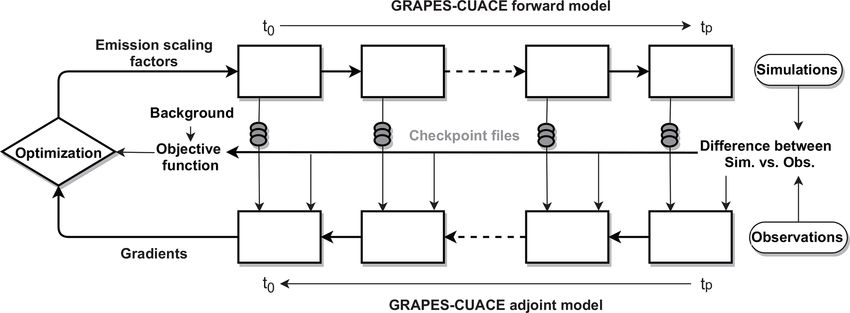
340                                         C. Wang et al.: Development of GRAPES–CUACE-4D-Var V1.0 and its application

ule into hourly gridded off-line data for 32 species, includ-              and the operator in Eq. (5) is the transpose of the opera-
ing BC, OC, SF, NI, fugitive dust particles and 19 non-                    tor in Eq. (4) (Liu, 2005). It is easy to see that the gradi-
methane volatile organic compounds (VOCs), CH4 , NH3 ,                     ent (sensitivity) of the objective function with respect to in-
CO, CO2 , SOx and NOx , at three vertical levels (non-point                put variables can be obtained through n times TLM simu-
source on the ground, middle-elevation point source at 50 m                lations or m times adjoint simulations. When n  m (such
and high-elevation point source at 120 m), as required by the              as n-dimensional emission sources and m-dimensional pollu-
GRAPES–CUACE model. Furthermore, natural sea salt and                      tant concentrations), the calculation efficiency of the adjoint
natural sand or dust emissions were also calculated online in              model is much higher than that of the TLM (Liu, 2005).
the model (Zhou et al., 2012; Zhai et al., 2018).
                                                                           2.2.2   GRAPES–CUACE aerosol adjoint
2.2       Adjoint model
                                                                           The GRAPES–CUACE aerosol adjoint model was con-
2.2.1        Adjoint theory                                                structed by An et al. (2016) based on the adjoint theory (Ye
                                                                           and Shen, 2006; Liu, 2005) and the CUACE aerosol mod-
Assuming that L is a linear operator defined in the Hilbert                ule, which mainly includes the adjoint of physical and chem-
space H, if there is another linear operator L∗ satisfying                 ical processes and flux calculation processes of six types of
                                                                           aerosols (SF, NI, SS, BC, OC and SD) in the CAM mod-
∀x, y ∈ H, (Lx, y) = (x, L∗ y).                                     (1)    ule, the adjoint of interface programs that connect GRAPES-
                                                                           Meso and CUACE, and the adjoint of aerosol transport pro-
Then L∗ is called the adjoint operator of L (Ye and Shen,
                                                                           cesses.
2006). Where (., .) denotes the inner product in H. If x, y
                                                                              As described in An et al. (2016), after the construction of
are continuous functions    R on a domain , the inner product             the adjoint model is completed, its accuracy must be verified
is defined as (x, y) =  x · yd; if x, y are discrete vectors,
                                                                           to confirm its reliability. Since the adjoint model is built on
x = [x1 x2 , . . ., xN ], y = [y1 y2 , . . ., yN ], then the inner prod-
                     N
                                                                           the basis of the TLM, the validity of the TLM must be en-
                                                                           sured before the accuracy of the adjoint model is tested. The
                    P
uct is (x, y) =         xi ·yi . When x and y denote vectors and L
                     i=1                                                   verification formula of tangent linear codes can be expressed
is a matrix (independent of x and y), we can obtain                        as
(Lx, y) = y T Lx = x T LT y = (x, LT y).                            (2)              F (X + δX) − F(X)
                                                                           Index =                     = 1.0,                            (6)
                                                                                          δXF0 (X)
In other words, for a matrix-type linear operator, the adjoint
operator is its transpose: L∗ = LT (Liu, 2005).                            where the denominator is the TLM output, and the numera-
   An atmospheric chemistry model can be viewed as a nu-                   tor is the difference between the output value of the original
merical operator F : R n → R m , which can be expressed as                 model with input X + δX and input X. It is necessary to de-
                                                                           crease the value of δX by an equal ratio and repeat the cal-
Y = F(X),                                                           (3)    culation of the above formula. If the result approaches 1.0,
                                                                           the tangent linear codes are correct. It was verified that all
where X ∈ R n and Y ∈ R m are vectors representing the input               input variables in the model, such as the concentration value
and output variables in the atmospheric chemistry model, re-               of pollutants (xrow) and the particle’s wet radius (rhop), have
spectively. If F is differentiable, then the differential of Y             passed the TLM test.
(δY ) can be denoted by the differential of X (δX), and the                   The adjoint codes can be validated on the basis of the cor-
tangent linear model (TLM) of the atmospheric chemistry                    rect tangent linear codes. The adjoint codes and the tangent
model can be expressed as                                                  linear codes need to satisfy Eq. (2) for all possible combina-
                                                                           tions of X and Y . In Eq. (2), L and L∗ represent the tangent
δY = ∇X F · δX,                                                     (4)    linear process and the adjoint process, respectively. To sim-
                                                                           plify the testing process, the adjoint input is the tangent linear
where δX ∈ R n and δY ∗ ∈ R m are input and output variables               output: Y = L(X). Thus, Eq. (5) can be expressed as
in the TLM, respectively, and ∇ X F is the Jacobian matrix.
   According to Eqs. (1) and (2), the adjoint model of the                 (∇F · dX, ∇F · dX) = (dX, ∇ T F(∇F · dX)).                    (7)
TLM can be expressed as
                                                                           By substituting dX into the tangent linear codes, the output
δX    ∗
          = ∇ TX F · δY ∗ ,                                         (5)    value ∇F · dX can be obtained and the left part of the equa-
                                                                           tion can be computed. Then, taking ∇F · dX as the input of
where δY ∗ ∈ R m and δX∗ ∈ R n are input and output vari-                  the adjoint codes, the adjoint output ∇ T F(∇F · dX) can be
ables in the adjoint model, respectively. Comparing Eqs. (4)               obtained and the right part of the equation can be calculated.
and (5), it can be seen that the dimensions of input and out-              On condition that the left and right sides of Eq. (7) are equal
put are exchanged between the TLM and the adjoint model,                   within the range of machine errors, the constructed adjoint

Geosci. Model Dev., 14, 337–350, 2021                                                        https://doi.org/10.5194/gmd-14-337-2021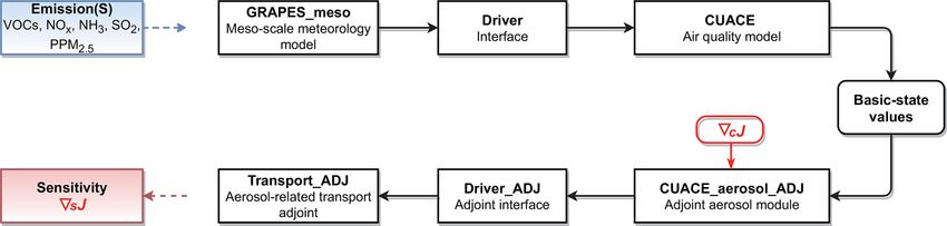
C. Wang et al.: Development of GRAPES–CUACE-4D-Var V1.0 and its application                                                      341

model is validated. It was verified that all input variables in     tion to the Hessian is updated. The limited memory BFGS
the model have passed the adjoint test. Taking the pollutant        matrix is used to define a quadratic model of the objective
concentration variable (xrow) as an example, both sides of          function f . A search direction d k is computed by a two-stage
Eq. (7) produce values with 14 identical significant digits or      approach. First, use the gradient projection method to iden-
more. This result is within the range of machine errors, so         tify a set of active variables, such as variables that will be
the values of the left and the right sides are considered equal.    held at their bounds. Then, the quadratic model is approx-
Thus, the pollutant concentration variable (xrow) has passed        imately minimized with respect to the free variables. The
the adjoint test.                                                   search direction is defined to be the vector leading from the
   After the TLM and the adjoint model were verified, the           current iterate to this approximate minimizer. Finally, a line
GRAPES–CUACE aerosol adjoint model was constructed.                 search is performed along the search direction d k to com-
The operation flowchart of the adjoint model is shown in            pute a step length λk , and the variables are updated through
Fig. 1. J is the objective function, which can be defined ac-       x k+1 = x k + λk d k . The L-BFGS-B algorithm has three ter-
cording to the problems concerned. c and s represent state          mination criteria: the number of iterations reaches the set
variables (such as BC concentration) and control variables          maximum value; the change of the objective function in con-
(such as emission sources, mainly including VOCs, NOx ,             secutive iterations is relatively small; and the modulus of the
NH3 , SO2 and PPM2.5 ) in the model, respectively. First of all,    projected gradient is small enough.
the GRAPES–CUACE atmospheric chemistry model should
be integrated to store the basic-state values of the unequi-
librated variables in checkpoint files. The intermediate val-       3     Description of GRAPES–CUACE-4D-Var
ues are recalculated or saved in stack using the PUSH&POP
method, which pushes the intermediate values into a contin-         The new 4D-Var data assimilation system, GRAPES–
uous memory space and pops them out where needed, during            CUACE-4D-Var, was constructed on the basis of the
the adjoint operating process. Subsequently, the gradient of J      GRAPES–CUACE atmospheric chemistry model, the
with respect to c (∇c J ) as well as the saved basic-state values   GRAPES–CUACE aerosol adjoint model and the L-BFGS-B
are taken as input data for the adjoint backward integration.       method. A schematic diagram of GRAPES–CUACE-4D-Var
Finally, the sensitivity of J with respect to s (∇s J ) can be      is shown in Fig. 2. The main parts of GRAPES–CUACE-
obtained. A full description of the construction, framework         4D-Var include GRAPES–CUACE atmospheric chemistry
and operational flowchart of the GRAPES–CUACE aerosol               simulation, during which the basic-state values of the unequi-
adjoint model can be found in An et al. (2016).                     librated variables in checkpoint files are saved, observations
                                                                    and adjoint forcing term processing, GRAPES–CUACE
2.3   L-BFGS-B method                                               aerosol adjoint model simulation, gradient extraction,
                                                                    cost function calculation, and optimization. The details of
The limited-memory Broyden–Fletcher–Goldfarb–Shanno                 cost function, observations and optimization of emission
algorithm (L-BFGS) is an optimization algorithm in the fam-         inversion are as follows.
ily of quasi-Newton methods that approximates the BFGS
using a limited amount of computer memory (Liu and No-              3.1    Cost function
cedal, 1989). The L-BFGS-B algorithm extends L-BFGS to
solve large nonlinear optimization problems subject to sim-         Based on Bayesian theory and the assumption of Gaussian
ple bounds on the variables (Byrd et al., 1995; Zhu et al.,         error distributions (Rodgers, 2000) the cost function of the
1997), which can be expressed as                                    emission inversion is generally defined as follows:
minf (x) , x ∈ R n ,                                        (8a)             1
                                                                    J (x) = γ (x − x b )T B−1 (x − x b )
subject to l ≤ x ≤ u,                                       (8b)             2
                                                                             p
where f is a nonlinear function, the vectors l and u represent            1 X               T
                                                                                Fi (x) − y i R−1 Fi (x) − y i ,

                                                                       +                                                          (9)
lower and upper bounds on the variables, and the number of                2 i=0
variables n is assumed to be large. The algorithm is also ap-
propriate and efficient for solving unconstrained problems in       where x, which we sought to optimize, generally represents
which the variables have no bounds. With the supply of the          the state vector of emissions or their scaling factors, x b is the
objective function f and its gradient g, but with no require-       prior estimate of x, B is the error covariance estimate of x b ,
ment of knowledge about the Hessian matrix of the objec-            F is the forward model, y is the vector of measurements that
tive function f , the algorithm can be useful for solving large     are distributed during the time interval [t0 , tp ], R is the ob-
problems where the Hessian matrix is difficult to compute or        servation error covariance matrix, and γ is the regularization
is dense.                                                           parameter.
   The brief procedure of the L-BFGS-B algorithm is as fol-            In this study, we followed the method in Henze et
lows. At each iteration, a limited memory BFGS approxima-           al. (2009), and defined x as the state vector of scaling fac-

https://doi.org/10.5194/gmd-14-337-2021                                                    Geosci. Model Dev., 14, 337–350, 2021
342 C. Wang et al.: Development of GRAPES–CUACE-4D-Var V1.0 and its application
Figure 1. Running process of GRAPES–CUACE atmospheric chemistry model and its adjoint model.
Figure 2. GRAPES–CUACE-4D-Var assimilation system.
tors of BC emissions: over China in 2004 and had 54 monitoring stations in the
summer of 2016. The monitoring of BC was conducted
s
x = ln , (10) by an aethalometer (Model AE 31, Magee Scientific Co.,
sb
USA), which uses a continuous optical greyscale measure-
where s is the state vector of the daily gridded emissions of ment method to produce real-time BC data (Gong et al.,
BC at three vertical levels (non-point source on the ground, 2019). In this study, we used the recommended mass ab-
middle-elevation point source at 50 m and high-elevation sorption coefficient for the instrument at an 880 nm wave-
point source at 120 m) and s b is the prior estimate of s. Thus, length with 24 h mean values of BC during 1–31 July 2016
the prior estimate of x(x b ) is equal to 0. According to Cao at five representative stations of CAWNET in northern China
et al. (2011), the uncertainty of prior BC emissions used in (Fig. S1 in the Supplement).
this study is 76.2 %. Therefore, we assigned the prior error The surface PM2.5 concentrations were obtained from
covariance matrix (B) to be diagonal and the uncertainty to the public website of the China Ministry of Ecology and
be 76.2 % for BC emissions. Due to the lack of informa- Environment (MEE) (http://www.mee.gov.cn/, last access:
tion to completely construct a physically representative B, 14 January 2021). The network started to release real-time
the regularization parameter γ is introduced to balance the hourly concentrations of SO2 , NO2 , CO, ozone (O3 ), PM2.5
background and observation terms in the cost function. As and PM10 in 74 major Chinese cities in January 2013, which
described in Henze et al. (2009), an optimal value of γ can further increased to 338 cities in 2016. The PM2.5 data were
be found with the L-curve method (Hansen, 1998). Here, we collected by the TEOM1405-F monitor, which draws ambi-
followed this method and obtained γ = 0.0001 through sev- ent air through a sample filter at constant flow rate, contin-
eral emission inversions with a range of γ (10, 1, 0.1, 0.01, uously weighing the filter and calculates the near real-time
0.001, 0.0001, 0.00001, 0.000001, 0.0000001). mass concentration of the collected particulate matter. We
3.2 Observations used hourly surface PM2.5 concentrations for 1–31 July 2016
at 48 cities in northern China, including 12 cities in the
The surface measurements of BC were collected from Beijing–Tianjin–Hebei region (Fig. S1). Here, we have av-
the China Atmosphere Watch Network (CAWNET). The eraged PM2.5 concentrations at several monitoring sites in
CAWNET was established by the China Meteorological Ad- each city to represent a regional condition.
ministration to monitor the BC surface mass concentration
Geosci. Model Dev., 14, 337–350, 2021 https://doi.org/10.5194/gmd-14-337-2021C. Wang et al.: Development of GRAPES–CUACE-4D-Var V1.0 and its application 343
To improve the performance of emission inversion, ade-
quate observations are needed for constraining the model.
Due to the limited BC monitoring sites in northern China, we
used the surface PM2.5 concentrations at 48 cities described
above and the BC/PM2.5 ratio to obtain the hourly BC con-
centrations for 1–31 July 2016 at 48 cities in northern China.
The detailed calculation process can be found in the Supple-
ment.
The observation error covariance matrix (R), which is dif-
ficult to quantify, generally includes contributions from the
measurement error, the representation error and the forward
model error (Henze et al., 2009; Zhang et al., 2016; Cao et
al., 2018). And there is also a certain error in calculating the
BC concentration based on the BC/PM2.5 ratio. To reflect the
possibly large uncertainties of the observation, we assumed
Figure 3. Cost function reduction.
R to be diagonal and with error of 100 %.
3.3 Optimization
than 1 % in consecutive iterations. According to the maxi-
Minimization of the cost function Eq. (9) is performed mum estimation range of the prior emissions, here the upper
through optimization. Starting from an initial guess (x equal and lower bounds of the scaling factors of BC emissions are
to 0), the forward model simulates BC concentrations at each ln(1.6) and ln(0.4), respectively.
integration step during the time interval [t0 , tp ], and the ad-
joint model, which is driven by the discrepancy between sim-
ulated and observed BC concentrations, calculates the gra- 4 Results and discussion
dients of the cost function with respect to the scaling fac-
tors of BC emission (Fig. 2). Subsequently, the gradients are 4.1 Comparisons between the simulated and observed
supplied to the L-BFGS-B optimization routine (Byrd et al., concentrations
1995; Zhu et al., 1997) to minimize the cost function itera-
tively (Fig. 2). At each iteration, the improved estimates of The progression of the cost function at iteration k (Jk /J0 )
the scaling factors are implemented and the forward and ad- during the optimization procedure is shown in Fig. 3. The
joint models are integrated. cost function quickly reduces and reaches the convergence
criterion after eight iterations, with values of the converged
3.4 Setup of emission inversion experiment cost function reduced by 37 %.
Figure 4 shows the spatial distribution of observed and
The simulation domain in this study is northern China (105– simulated daily BC concentrations on 4 July 2016. In gen-
125◦ E, 32.25–43.25◦ N; Fig. S1), covering 41 × 23 horizon- eral, the results simulated with the prior emission reflect the
tal grids with a resolution of 0.5◦ ×0.5◦ and vertically divided distribution characteristics of BC concentration in northern
into 31 layers with an integration time step of 300 s. The China to a certain extent, with high values mainly located
National Centers for Environmental Prediction Final (FNL) in Beijing and central and southern Hebei and low values
Analysis dataset at a 6 h interval is used as meteorologi- mainly located in Inner Mongolia and eastern Shandong.
cal input. The prior emission used here is the daily grid- However, the differences between the simulated and the ob-
ded BC emission at three vertical levels (non-point source served BC concentrations are considerable, and almost all are
on the ground, middle-elevation point source at 50 m and over-predictions. The optimized (posterior) emissions com-
high-elevation point source at 120 m) mentioned above. The pensate for the over-predictions and largely reduce the model
results calculated by the BC/PM2.5 ratio show that the BC biases. For instance, the model biases for BC in Beijing,
concentration in Beijing was high on 4 July 2016. So the as- Tianjin, Shijiazhuang, Jinan, Taiyuan and Zhengzhou are re-
similation window is from 20:00 CST, 3 July, to 19:00 CST, duced by 46 % (from 5.4 to 2.9 µg/m3 ), 26 % (from 6.6 to
4 July 2016. The hourly BC concentrations at 36 cities dur- 4.9 µg/m3 ), 29 % (from 18.4 to 13.1 µg/m3 ), 20 % (from 6.6
ing this time interval are used for the emission inversion, and to 5.3 µg/m3 ), 34 % (from 4.1 to 2.7 µg/m3 ) and 20 % (from
the BC concentrations of the remaining 12 cities are used 6.9 to 5.5 µg/m3 ), respectively (Fig. 4a, b). The results simu-
for validation of the inversion effect (Fig. S1). The simula- lated with the optimized emission also show improved agree-
tion is initialized at 20:00 CST, 30 June; the first 3 d are set ment with the observations over northern China with lower
as the spin-up time. The convergence criterion used in the root-mean-square errors and higher correlation coefficients
optimization is that the objective function decreases by less (Fig. 4a, b).
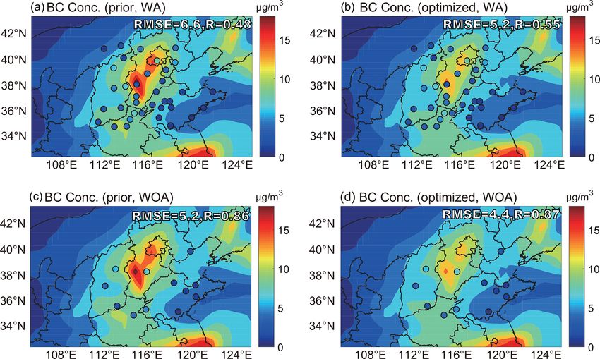
https://doi.org/10.5194/gmd-14-337-2021 Geosci. Model Dev., 14, 337–350, 2021344 C. Wang et al.: Development of GRAPES–CUACE-4D-Var V1.0 and its application
Figure 4. The spatial distribution of observed and simulated daily BC concentrations on 4 July 2016. The observations (circles) are over-
plotted over model simulations with the (a, c) prior and (b, d) optimized emissions. The observations at 36 cities in (a) and (b) were used in
the assimilation, and the observations at 12 cities in (c) and (d) were not used in the assimilation. The root-mean-square error (RMSE) and
correlation coefficient (R) between observation and simulation are shown as insets. The observed BC concentrations were calculated by the
BC/PM2.5 ratio method.
It is crucial to validate the assimilation results by observa- (Fig. 5b, d, f). However, the optimized emissions are con-
tions that were not utilized in the assimilation. The BC con- siderably reduced (Fig. 5b, d, f). Especially for the regions
centrations at 12 cities were used for validation (Fig. 4c, d). where observation sites are located, such as southern Beijing,
Assimilation compensates for over-predictions, reduces the Tianjin, central and southern Hebei, northwest Shandong,
root-mean-square errors (from 5.2 to 4.4) and improves the central Shanxi, and northern Henan, BC emissions decrease
correlation coefficients (from 8.6 to 8.7). The model biases significantly. As for the regions where observation sites are
for BC in Hengshui and Yizhou are reduced by 28 % (from not located, such as Liaoning and Jiangsu, BC emissions are
7.2 to 5.2 µg/m3 ) and 36 % (from 3.9 to 2.5 µg/m3 ), respec- almost unchanged. The reason for this phenomenon is dis-
tively. The improvements of the remaining 10 cities are also cussed in Sect. 4.3.
notable, with values of the model biases reduced by 1 %– In order to analyse the differences between the prior and
20 %. optimized BC emissions in Beijing–Tianjin–Hebei–Shanxi–
Shandong–Henan region in more depth and detail, we calcu-
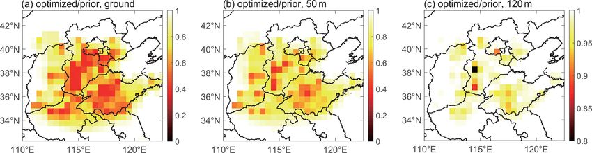
4.2 Comparisons between the prior and optimized BC lated the ratio of the optimized emissions to prior emissions
emissions (optimized emissions divide by prior emissions), as shown
in Fig. 6. In general, assimilation has the largest reduction
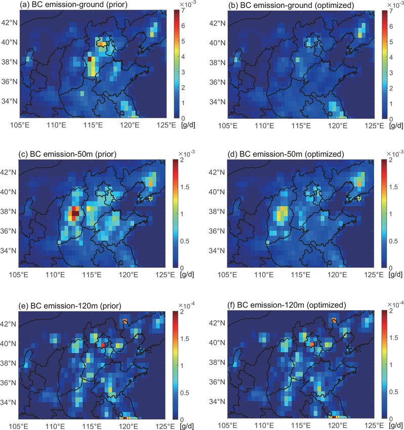
Figure 5 shows the spatial distributions of the prior and op- in the non-point source on the ground (Fig. 6a), followed by
timized daily BC emissions, which are at three vertical lev- the middle-elevation point source at 50 m (Fig. 6b), and the
els (non-point source on the ground, middle-elevation point smallest reduction in the high-elevation point source at 120 m
source at 50 m and high-elevation point source at 120 m) (Fig. 6c). This is related to the intensity of BC emissions at
as required by the GRAPES–CUACE model. The BC emis- three vertical levels. The intensity of BC emissions on the
sions on the ground are mostly non-point sources and at 50 m ground (Fig. 5a) is about 1–2 orders of magnitude higher than
are concentrated middle-elevation sources; therefore they are that of the middle-elevation point source at 50 m (Fig. 5c) and
distributed in a large area (Fig. 5a, c), while the BC emissions the high-elevation point source at 120 m (Fig. 5e). In other
at 120 m are mainly from a few high-elevation point sources, words, the BC emissions on the ground have the most signif-
so they are scattered in the area (Fig. 5e). It can be seen that icant effect on the overall cost function and therefore reduced
the distributions of optimized BC emissions at three vertical most during the progression of assimilation.
levels are relatively consistent with those of prior emissions
Geosci. Model Dev., 14, 337–350, 2021 https://doi.org/10.5194/gmd-14-337-2021C. Wang et al.: Development of GRAPES–CUACE-4D-Var V1.0 and its application 345 Figure 5. Spatial distributions of the (a, c, e) prior and (b, d, f) optimized daily BC emissions. The emissions are at three vertical levels: (a, b) non-point source on the ground, (c, d) middle-elevation point source at 50 m and (e, f) high-elevation point source at 120 m, as required by the GRAPES–CUACE model. Figure 6. The ratio of optimized emissions to prior emissions (optimized emissions divide by prior emissions). (a) Non-point source on the ground, (b) middle-elevation point source at 50 m and (c) high-elevation point source at 120 m. https://doi.org/10.5194/gmd-14-337-2021 Geosci. Model Dev., 14, 337–350, 2021
346                                              C. Wang et al.: Development of GRAPES–CUACE-4D-Var V1.0 and its application

Table 1. Anthropogenic BC emissions in China by province in
2006a and 2016b (units: Gg/year).

            Province                2006                   2016
            Beijing               19.00           7.70 (0.41)
            Tianjin               15.00          10.81 (0.72)
            Hebei                137.00          97.99 (0.72)
            Shanxi               139.00          69.26 (0.50)
            Shandong             132.00         108.82 (0.82)
            Henan                133.00          82.42 (0.62)
            Total China        1811.00        1315.28 (0.73)
          Note: numbers in parentheses represent emission ratios
          relative to 2006. a Source: Zhang et al. (2009). b Source:    Figure 7. Comparison of observed and simulated (with the prior
          MEIC (Multi-resolution Emission Inventory for China),         and optimized BC emissions, respectively) BC concentrations in
          http://meicmodel.org/ (last access: 14 January 2021).
                                                                        Beijing from 20:00, 3 July, to 19:00, 4 July 2016. The observed
                                                                        BC concentrations were calculated by the BC/PM2.5 ratio method.

   The prior BC emissions used in this study are based on
statistical data of anthropogenic emissions for 2007 (Cao et
al., 2011), and the BC observations used for assimilation are           observations (5.7 µg/m3 ). With such a high initial concentra-
from 2016, so the ratios of the optimized emissions to prior            tion, the simulated BC concentrations with prior emissions
emissions can reflect the changes in BC emissions from 2007             were significantly higher than the observed concentrations
to 2016 to a certain extent. From the perspective of each               at all times. The simulations with optimized emissions com-
province, we can see that the ratios of the optimized emis-             pensated for the over-predictions, but the BC concentrations
sions to prior emissions in Beijing, Tianjin, Hebei, Shanxi,            were still higher than the observations in the first few hours
Shandong and Henan are 0.4–0.8, 0.4–0.7, 0.4–0.8, 0.6–0.8,              (from 20:00, 3 July, to 02:00, 4 July 2016). And the model
0.4–0.8 and 0.5–0.8, respectively. This indicates that the BC           bias during this time period was 5.2 µg/m3 . As the influence
emissions in these highly industrialized regions have greatly           of the initial concentration on the simulation gradually weak-
reduced from 2007 to 2016, which is consistent with previous            ened, the simulated BC concentrations with optimized emis-
studies (Zheng et al., 2018). Table 1 lists the anthropogenic           sions were largely reduced and much closer to the observa-
BC emissions in China by province in 2006 and 2016 and the              tions from 03:00 to 19:00, 4 July 2016, and the model bi-
emission ratios of 2016 relative to 2006. According to pre-             ases during this time period also decreased, with the value of
vious research, the emission ratios of 2016 relative to 2006            1.9 µg/m3 . This indicates that for short-term simulation, the
are 0.41–0.82 in Beijing–Tianjin–Hebei–Shanxi–Shandong–                 influence of initial concentration on the simulation is not neg-
Henan region and 0.73 over China. It can be seen that the ra-           ligible. In further work, it is also of great significance to use
tios of the optimized emissions to prior emissions calculated           the GRAPES–CUACE-4D-Var assimilation system to opti-
in this study are within a reasonable range, which also shows           mize the initial concentration to improve the simulation ef-
that the newly constructed GRAPES–CUACE-4D-Var as-                      fect.
similation system can obtain reasonable BC emissions based                 As described in Sect. 4.2, after assimilation, the BC emis-
on the observations.                                                    sions in the regions where observation sites are located de-
                                                                        crease significantly, while in the regions where observation
4.3   Discussion                                                        sites are not located, such as Liaoning and Jiangsu, BC emis-
                                                                        sions are almost unchanged. This may be due to the short
Although Sect. 4.1 shows that assimilation reduces the model            period of the observation data used for assimilation. In this
biases and improves all statistical values at each site, there          study, since the GRAPES–CUACE-4D-Var assimilation sys-
are still over-predictions to a certain degree. In addition to          tem has not yet implemented parallel computing, the assim-
the emission, the initial concentration is also an important            ilation window was set for 24 h. In such a short period of
factor that affects the BC simulation. Here, we take Beijing            time, the pollutants emitted from Liaoning and Jiangsu may
as an example to analyse the influence of the initial con-              not have been transported to the regions where observation
centration on the BC simulation. Figure 7 shows the com-                sites are located, thus having little impact on the BC concen-
parison of observed and simulated (with the prior and opti-             trations in these regions. In other words, the emissions from
mized BC emissions, respectively) BC concentrations in Bei-             Liaoning and Jiangsu have little effect on the overall cost
jing from 20:00, 3 July, to 19:00, 4 July 2016. At the initial          function, so there is little change during the progression of
moment (20:00, 3 July 2016), the initial concentration for              assimilation. Therefore, implementing parallel computing of
simulation (11.5 µg/m3 ) was about 2 times higher than the              the GRAPES–CUACE-4D-Var assimilation system and per-

Geosci. Model Dev., 14, 337–350, 2021                                                     https://doi.org/10.5194/gmd-14-337-2021
C. Wang et al.: Development of GRAPES–CUACE-4D-Var V1.0 and its application 347
forming emission inversion for a longer period (i.e. 1 month) of emission reduction are crucial for formulating optimized
is another important task in the future. pollution-control strategies for PM2.5 and O3 in China.
5 Conclusions Code and data availability. The GRAPES–CUACE atmospheric
chemistry model used in this study was distributed by the Na-
In this study, we developed a new 4D-Var data assimila- tional Meteorological Center of the Chinese Meteorology Ad-
tion system for the GRAPES–CUACE atmospheric chem- ministration (2021, http://www.nmc.cn) together with the Insti-
istry model (GRAPES–CUACE-4D-Var) and applied it for tute of Atmospheric Composition and Environmental Meteorol-
assimilating surface BC concentrations and optimizing its ogy of the Chinese Academy of Meteorological Sciences (2021,
daily emissions in northern China on 4 July 2016, when a http://www.camscma.cn). The model was run on an IBM Pure-
Flex System (AIX) with an XL Fortran Compiler. The code of
pollution event occurred in Beijing. The main conclusions
the GRAPES–CUACE aerosol adjoint model is available online
are as follows. at https://doi.org/10.5194/gmd-9-2153-2016-supplement (An et al.,
2016). The code of GRAPES_CUACE_4D_Var_driver.F can be
– The newly constructed GRAPES–CUACE-4D-Var as-
downloaded as a Supplement to this article. The observations are
similation system is feasible and can be applied to per- available online at http://www.mee.gov.cn/ (Ministry of Ecology
form BC emission inversion in northern China. and Environment of the People’s Republic of China, 2021).
– The BC concentrations simulated with optimized emis-
sions show improved agreement with the observations Supplement. The supplement related to this article is available on-
over northern China with lower root-mean-square errors line at: https://doi.org/10.5194/gmd-14-337-2021-supplement.
and higher correlation coefficients. The model biases
are reduced by 20 %–46 %. The validation of assimi-
lation results with observations that were not utilized Author contributions. XA envisioned and oversaw the project. XA
in the assimilation shows that assimilation compensates and CW designed and developed the GRAPES–CUACE-4D-Var as-
for over-predictions, reduces the root-mean-square er- similation system and prepared the paper. CW designed the exper-
rors and improves the correlation coefficients. The im- iments and carried out the simulations with contributions from all
provements are also notable, with values of the model other co-authors. QH and ZS provided the observation data used
biases reduced by 1 %–36 %. in the study. YL and JL processed the data and prepared the data
visualization. All authors reviewed the paper.
– Compared with the prior BC emissions, the optimized
emissions are considerably reduced. Especially for Bei-
jing, Tianjin, Hebei, Shandong, Shanxi and Henan, the Competing interests. The authors declare that they have no conflict
ratios of the optimized emissions to prior emissions are of interest.
0.4–0.8, indicating that the BC emissions in these highly
industrialized regions have greatly reduced from 2007
Acknowledgements. We thank Lin Zhang from the Numerical Fore-
to 2016, which is consistent with previous studies.
cast Center of the China Meteorological Administration for provid-
In the following work, implementing parallel computing of ing technical support with the optimization algorithm.
the GRAPES–CUACE-4D-Var assimilation system and per-
forming emission inversion for a longer period is an impor-
Financial support. This research has been supported by the Na-
tant task. Apart from the emissions, the initial concentration
tional Key Research and Development Program of China (grant no.
is also an important factor for short-term simulation. It is of 2017YFC0210006) and the National Natural Science Foundation of
great significance to use the GRAPES–CUACE-4D-Var as- China (grant nos. 41975173 and 91644223).
similation system to optimize the initial concentration to im-
prove the simulation effect.
Meanwhile, several mega urban agglomerations in China Review statement. This paper was edited by Augustin Colette and
are facing atmospheric compound pollution with high PM2.5 reviewed by two anonymous referees.
and O3 concentrations (Li et al., 2019; Zhang et al., 2019; Xi-
ang et al., 2020; Haque et al., 2020; Zhao et al., 2020). To im-
prove air quality, it is urgent to formulate reasonable and ef-
fective emission-reduction measures. Therefore, further stud-
ies on expanding the function of the GRAPES–CUACE-4D-
Var assimilation system and taking into account factors such
as air quality standards, the proportion of emissions that can
be reduced, the economic cost and residents’ health benefits
https://doi.org/10.5194/gmd-14-337-2021 Geosci. Model Dev., 14, 337–350, 2021348 C. Wang et al.: Development of GRAPES–CUACE-4D-Var V1.0 and its application
References Elbern, H., Strunk, A., Schmidt, H., and Talagrand, O.: Emis-
sion rate and chemical state estimation by 4-dimensional
variational inversion, Atmos. Chem. Phys., 7, 3749–3769,
An, X. Q., Zhai, S. X., Jin, M., Gong, S., and Wang, Y.: Devel- https://doi.org/10.5194/acp-7-3749-2007, 2007.
opment of an adjoint model of GRAPES–CUACE and its ap- Gong, S. L. and Zhang, X. Y.: CUACE/Dust – an integrated
plication in tracking influential haze source areas in north China, system of observation and modeling systems for operational
Geosci. Model Dev., 9, 2153–2165, https://doi.org/10.5194/gmd- dust forecasting in Asia, Atmos. Chem. Phys., 8, 2333–2340,
9-2153-2016, 2016. https://doi.org/10.5194/acp-8-2333-2008, 2008.
Andre, J. C., Demoor, G., Lacarrere, P., Therry, G., and Du- Gong, S. L., Barrie, L. A., Blanchet, J.-P., Salzen, K. V., Lohmann,
vachat, R.: Modeling the 24-hour evolution of the mean U., Lesins, G., Spacek, L., Zhang, L. M., Girard, E., and Lin,
and turbulent structures of the planetary boundary layer, H.: Canadian Aerosol Module: A size-segregated simulation
J. Atmos. Sci., 35, 1861–1883, https://doi.org/10.1175/1520- of atmospheric aerosol processes for climate and air quality
0469(1978)0352.0.Co;2, 1978. models, 1, Module development, J. Geophys. Res., 108, 4007,
Betts, A. K. and Miller, M. J.: A new convective adjustment scheme https://doi.org/10.1029/2001JD002002, 2003.
Part II: Single column tests using GATE wave, BOMEX, and Gong, T., Sun, Z., Zhang X., Zhang, Y., Wang, S., Han,
arctic air-mass data sets, Q. J. Roy. Meteor. Soc., 112, 693–709, L., Zhao, D., Ding, D., and Zheng, C.: Associations of
https://doi.org/10.1002/qj.49711247308, 1986. black carbon and PM2.5 with daily cardiovascular mor-
Byrd, R. H., Lu, P., Nocedal, J., and Zhu, C.: A limited memory al- tality in Beijing, China, Atmos. Environ., 214, 116876,
gorithm for bound constrained optimization, SIAM J. Sci. Com- https://doi.org/10.1016/j.atmosenv.2019.116876, 2019.
put., 16, 1190–1208, https://doi.org/10.1137/0916069, 1995. Hakami, A., Henze, D. K., Seinfeld, J. H., Chai, T., Tang, Y.,
Cao, G. L., Zhang, X. Y., Gong, S. L., An, X. Q., and Carmichael, G. R., and Sandu, A.: Adjoint inverse modeling of
Wang, Y. Q.: Emission inventories of primary particles and black carbon during the Asian Pacific Regional Aerosol Charac-
pollutant gases for China, Chinese Sci. Bull., 56, 781–788, terization Experiment, J. Geophys. Res.-Atmos., 110, D14301,
https://doi.org/10.1007/s11434-011-4373-7, 2011. https://doi.org/10.1029/2004JD005671, 2005.
Cao, H., Fu, T.-M., Zhang, L., Henze, D. K., Miller, C. C., Lerot, Hakami, A., Henze, D. K., Seinfeld, J. H., Singh, K.,
C., Abad, G. G., De Smedt, I., Zhang, Q., van Roozendael, M., Sandu, A., Kim, S., Byun, D., and Li, Q.: The ad-
Hendrick, F., Chance, K., Li, J., Zheng, J., and Zhao, Y.: Ad- joint of CMAQ, Environ. Sci. Technol., 41, 7807–7817,
joint inversion of Chinese non-methane volatile organic com- https://doi.org/10.1021/es070944p, 2007.
pound emissions using space-based observations of formalde- Hansen, P. C.: Rank-deficient and discrete ill-posed problems: nu-
hyde and glyoxal, Atmos. Chem. Phys., 18, 15017–15046, merical aspects of linear inversion, Society for Industrial and Ap-
https://doi.org/10.5194/acp-18-15017-2018, 2018. plied Mathematics, Philadelphia, USA, 1998.
Charney, J. G. and Phillips, N. A.: Numerical integration of the Haque, M. M., Fang, C., Schnelle-Kreis, J., Abbaszade, G.,
quasi-geostrophic equations for barotropic and simple baroclinic Liu, X. Y., Bao, M. Y., Zhang, W. Q., and Zhang, Y. L.:
flows, J. Meteorol., 10, 71–99, https://doi.org/10.1175/1520- Regional haze formation enhanced the atmospheric pol-
0469(1953)0102.0.CO;2, 1953. lution levels in the Yangtze River Delta region, China:
Chen, D., Xue, J., Yang, X., Zhang, H., Shen, X., Hu, J., Wang, Implications for anthropogenic sources and secondary
Y., Ji, L., and Chen, J.: New generation of multi-scale NWP sys- aerosol formation. Sci. Total Environ., 728, 138013,
tem (GRAPES): general scientific design, Chinese Sci. Bull., 53, https://doi.org/10.1016/j.scitotenv.2020.138013, 2020.
3433–3445, https://doi.org/10.1007/s11434-008-0494-z, 2008. Henze, D. K., Hakami, A., and Seinfeld, J. H.: Development of
Chen, F., Mitchell, K., Schaake, J., Xue, Y. K., Pan, H. L., Ko- the adjoint of GEOS-Chem, Atmos. Chem. Phys., 7, 2413–2433,
ren, V., Duan, Q. Y., Ek, M., and Betts, A.: Modeling of https://doi.org/10.5194/acp-7-2413-2007, 2007.
land surface evaporation by four schemes and comparison with Henze, D. K., Seinfeld, J. H., and Shindell, D. T.: Inverse model-
FIFE observations, J. Geophys. Res.-Atmos., 101, 7251–7268, ing and mapping US air quality influences of inorganic PM2.5
https://doi.org/10.1029/95jd02165, 1996. precursor emissions using the adjoint of GEOS-Chem, Atmos.
Dudhia, J.: Numerical study of convection observed Chem. Phys., 9, 5877–5903, https://doi.org/10.5194/acp-9-5877-
during the winter monsoon experiment using a 2009, 2009.
meso- scale two-dimensional model, J. Atmos. Hong, S. and Lim, J. J.: The WRF Single-Moment 6-Class Micro-
Sci., 46, 3077–3107, https://doi.org/10.1175/1520- physics Scheme (WSM6), Asia-pac. J. Atmos. Sci., 42, 129–151,
0469(1989)0462.0.CO;2, 1989. 2006.
Elbern, H. and Schmidt, H.: A four-dimensional variational chem- Hong, S. Y. and Pan, H. L.: Nonlocal boundary layer ver-
istry data assimilation scheme for Eulerian chemistry trans- tical diffusion in a medium-range forecast model, Mon.
port modeling, J. Geophys. Res.-Atmos., 104, 18583–18598, Weather Rev., 124, 2322–2339, https://doi.org/10.1175/1520-
https://doi.org/10.1029/1999JD900280, 1999. 0493(1996)1242.0.CO;2, 1996.
Elbern, H. and Schmidt, H.: Ozone episode analysis by four- dimen- Huang, S. X., Liu, F., Sheng, L., Cheng, L. J., Wu, L.,
sional variational chemistrydata assimilation. J. Geophys. Res.- and Li, J.: On adjoint method based atmospheric emis-
Atmos., 106, 3569–3590, 2001. sion source tracing, Chinese Sci. Bull., 63, 1594–1605,
Elbern, H., Schmidt, H., Talagrand, O., and Ebel, A.: 4D- https://doi.org/10.1360/N972018-00196, 2018.
variational data assimilation with an adjoint air qualitymodel Janjić, Z. I.: The step-mountain eta coordinate model:
for emission analysis, Environ. Modell. Softw., 15, 539–548, Further developments of the convection, viscous sub-
https://doi.org/10.1016/S1364-8152(00)00049-9, 2000.
Geosci. Model Dev., 14, 337–350, 2021 https://doi.org/10.5194/gmd-14-337-2021C. Wang et al.: Development of GRAPES–CUACE-4D-Var V1.0 and its application 349 layer, and turbulence closure schemes, Mon. Weather short-time forecasting, Atmos. Chem. Phys., 16, 3631–3649, Rev., 122, 927–945, https://doi.org/10.1175/1520- https://doi.org/10.5194/acp-16-3631-2016, 2016. 0493(1994)1222.0.CO;2, 1994. Resler, J., Eben, K., Jurus, P., and Liczki, J.: Inverse modeling of Jeong, J. I. and Park R J.: Efficacy of dust aerosol fore- emissions and their time profiles, Atmos. Pollut. Res., 1, 288– casts for East Asia using the adjoint of GEOS-Chem with 295, https://doi.org/10.5094/apr.2010.036, 2010. ground-based observations, Environ. Pollut., 234, 885–893, Rodgers, C. D.: Inverse methods for atmospheric sounding–Theory https://doi.org/10.1016/j.envpol.2017.12.025, 2018. and practice, Ser. on Atmos. Oceanic and Planet. Phys., Vol. 2, Jiang, Z., Jones, D. B. A., Worden, H. M., and Henze, D. K.: Sen- Singapore, https://doi.org/10.1142/9789812813718, 2000. sitivity of top-down CO source estimates to the modeled verti- Sandu, A., Daescu, D. N., Carmichael, G. R., and Chai, T.: Adjoint cal structure in atmospheric CO, Atmos. Chem. Phys., 15, 1521– sensitivity analysis of regional air quality models, J. Comput. 1537, https://doi.org/10.5194/acp-15-1521-2015, 2015. Phys., 204, 222–252, https://doi.org/10.1016/j.jcp.2004.10.011, Ke, H.: Construction and application of a real-time emission model 2005. of open biomass burning, Master dissertation, Chinese Academy Stockwell, W. R., Middleton, P., Change, J. S., and Tang, X.: of Meteorological Sciences, Beijing, 1–57, 2019 (in Chinese). The second generation regional acid deposition model chemical Kurokawa, J. I., Yumimoto, K., Uno, I., and Ohara, T.: mechanism for regional air quality modeling, J. Geophys. Res. Adjoint inverse modeling of NOx emissions over east- 95, 16343–16376, https://doi.org/10.1029/JD095iD10p16343, ern China using satellite observations of NO2 verti- 1990. cal column densities, Atmos. Environ., 43, 1878–1887, The Chinese Academy of Meteorological Sciences: Scientific https://doi.org/10.1016/j.atmosenv.2008.12.030, 2009. research, available at: http://www.camscma.cn/, last access: Li, K., Jacob, D. J., Liao, H., Shen, L., Zhang, Q., and Bates, K. 15 January 2021. H.: Anthropogenic drivers of 2013–2017 trends in summer sur- The National Meteorological Center: Numerical forecast, available face ozone in China, P. Natl. Acad. Sci. USA, 116, 422–427, at: http://www.nmc.cn/, last access: 15 January 2021. https://doi.org/10.1073/pnas.1812168116, 2019. Wang, C., An, X., Zhai, S., and Sun, Z.: Tracking a se- Liu, D. C. and Nocedal, J.: On the limited memory BFGS method vere pollution event in Beijing in December 2016 with the for large scale optimization, Math. Program., 45, 503–528, GRAPES-CUACE adjoint model, J. Meteorol. Res., 32, 49–59, https://doi.org/10.1007/BF01589116, 1989. https://doi.org/10.1007/s13351-018-7062-5, 2018a. Liu, F.: Adjoint model of Comprehensive Air quality Model CAMx Wang, C., An, X., Zhai, S., Hou, Q., and Sun, Z.: Tracking sen- – construction and application, Post-doctoral research report, sitive source areas of different weather pollution types using Peking University, Beijing, 1–101, 2005 (in Chinese). GRAPES-CUACE adjoint model, Atmos. Environ., 175, 154– Mao, Y. H., Li, Q. B., Henze, D. K., Jiang, Z., Jones, D. B. 166, https://doi.org/10.1016/j.atmosenv.2017.11.041, 2018b. A., Kopacz, M., He, C., Qi, L., Gao, M., Hao, W.-M., and Wang, C., An, X., Zhang, P., Sun, Z., Cui, M., and Ma, L.: Compar- Liou, K.-N.: Estimates of black carbon emissions in the west- ing the impact of strong and weak East Asian winter monsoon ern United States using the GEOS-Chem adjoint model, At- on PM2.5 concentration in Beijing, Atmos. Res., 215, 165–177, mos. Chem. Phys., 15, 7685–7702, https://doi.org/10.5194/acp- https://doi.org/10.1016/j.atmosres.2018.08.022, 2019. 15-7685-2015, 2015. Wang, H., Gong, S. L., Zhang, H. L., Chen, Y., Shen, X., Chen, D., Ministry of Ecology and Environment of the People’s Republic of Xue, J., Shen, Y., Wu, X., and Jin, Z.: A new-generation sand and China: Air Quality, available at: http://www.mee.gov.cn/, last ac- dust storm forecasting system GRAPES_CUACE/Dust: Model cess: 15 January 2021. development, verification and numerical simulation, Chinese Sci. Mlawer, E. J., Taubman, S. J., Brown, P. D., Iacono, M. Bull., 55, 635–649, https://doi.org/10.1007/s11434-009-0481-z, J., and Clough, S. A.: Radiative transfer for inhomoge- 2010. neous atmospheres: RRTM, a validated correlated-k model for Wang, H., Xue, M., Zhang, X. Y., Liu, H. L., Zhou, C. H., Tan, the longwave, J. Geophys. Res.-Atmos., 102, 16663–16682, S. C., Che, H. Z., Chen, B., and Li, T.: Mesoscale model- https://doi.org/10.1029/97JD00237, 1997. ing study of the interactions between aerosols and PBL mete- Monin, A. S. and Obukhov, A. M.: Basic laws of turbulent mixing orology during a haze episode in Jing–Jin–Ji (China) and its in the surface layer of the atmosphere, Contrib. Geophys. Inst. nearby surrounding region – Part 1: Aerosol distributions and Acad. Sci. USSR, 151, 163–187, 1954 (in Russian). meteorological features, Atmos. Chem. Phys., 15, 3257–3275, Müller, J.-F. and Stavrakou, T.: Inversion of CO and NOx emissions https://doi.org/10.5194/acp-15-3257-2015, 2015. using the adjoint of the IMAGES model, Atmos. Chem. Phys., 5, Wang, J., Xu, X., Henze, D. K., Zeng, J., Ji, Q., Tsay, S. C., 1157–1186, https://doi.org/10.5194/acp-5-1157-2005, 2005. and Huang, J.: Top-down estimate of dust emissions through Nenes, A., Pandis, S. N., and Pilinis, C.: ISORROPIA: A integration of MODIS and MISR aerosol retrievals with the new thermodynamic equilibrium model for multiphase multi- GEOS-Chem adjoint model, Geophys. Res. Lett., 39, L08802, component inorganic aerosols, Aquat. Geochem., 4, 123–152, https://doi.org/10.1029/2012GL051136, 2012. https://doi.org/10.1023/a:1009604003981, 1998a. West, J. J., Pilinis, C., Nenes, A., and Pandis, S. N.: Marginal di- Nenes, A., Pilinis, C., and Pandis, S.: Continued development and rect climate forcing by atmospheric aerosols, Atmos. Environ. testing of a new thermodynamics aerosol module for urban and 32, 2531–2542, https://doi.org/10.1016/s1352-2310(98)00003- regional air quality models, Atmos. Environ., 33, 1553–1560, x, 1998. https://doi.org/10.1016/S1352-2310(98)00352-5, 1998b. Xiang, S. L., Liu, J. F., Tao, W., Yi, K., Xu, J. Y. , Hu, X. Park, S. Y., Kim, D. H., Lee, S. H., and Lee, H. W.: Variational R., Liu, H. Z., Wang, Y. Q., Zhang, Y. Z., Yang, H. Z., Hu, data assimilation for the optimized ozone initial state and the J. Y., Wan, Y., Wang, X. J., Ma, J. M., Wang, X. L., and https://doi.org/10.5194/gmd-14-337-2021 Geosci. Model Dev., 14, 337–350, 2021
You can also read


