Ocean-forced evolution of the Amundsen Sea catchment, West Antarctica, by 2100
←
→
Page content transcription
If your browser does not render page correctly, please read the page content below
The Cryosphere, 14, 1245–1258, 2020
https://doi.org/10.5194/tc-14-1245-2020
© Author(s) 2020. This work is distributed under
the Creative Commons Attribution 4.0 License.

Ocean-forced evolution of the Amundsen Sea catchment,
West Antarctica, by 2100
Alanna V. Alevropoulos-Borrill1,a , Isabel J. Nias1,2,3 , Antony J. Payne1 , Nicholas R. Golledge4 , and Rory J. Bingham1
1 Centre for Polar Observation and Modelling, School of Geographical Sciences, University of Bristol,
University Road, Bristol, BS8 1SS, UK
2 Cryospheric Sciences Laboratory, NASA Goddard Space Flight Center, Greenbelt, MD, USA
3 Earth System Science Interdisciplinary Center, University of Maryland, College Park, MD, USA
4 Antarctic Research Centre, Victoria University of Wellington, Wellington, 6012, New Zealand
a now at: Antarctic Research Centre, Victoria University of Wellington, Wellington, 6012, New Zealand

Correspondence: Alanna V. Alevropoulos-Borrill (alanna.alevropoulosborrill@vuw.ac.nz)

Received: 29 August 2019 – Discussion started: 29 October 2019
Revised: 16 March 2020 – Accepted: 17 March 2020 – Published: 15 April 2020

Abstract. The response of ice streams in the Amundsen Sea            1   Introduction
Embayment (ASE) to future climate forcing is highly uncer-
tain. Here we present projections of 21st century response
of ASE ice streams to modelled local ocean temperature               The contribution of the Antarctic Ice Sheet is the greatest
change using a subset of Coupled Model Intercomparison               uncertainty in estimates of projected global mean sea level
Project (CMIP5) simulations. We use the BISICLES adap-               rise (Church et al., 2013; Schlegel et al., 2018). The Amund-
tive mesh refinement (AMR) ice sheet model, with high-               sen Sea Embayment (ASE) sector, West Antarctica, has been
resolution grounding line resolving capabilities, to explore         identified as a focal region for mass loss (McMillan et al.,
grounding line migration in response to projected sub-ice-           2014; Shepherd et al., 2012, 2018), draining one third of
shelf basal melting. We find a contribution to sea level rise        the West Antarctic Ice Sheet (Mouginot et al., 2014). Both
of between 2.0 and 4.5 cm by 2100 under RCP8.5 conditions            observational (Rignot et al., 2014; Smith et al., 2017) and
from the CMIP5 subset, where the mass loss response is lin-          modelling studies (Favier et al., 2014; Gladstone et al., 2012;
early related to the mean ocean temperature anomaly. To ac-          Golledge et al., 2019; Ritz et al., 2015) have inferred that the
count for uncertainty associated with model initialization, we       region is susceptible to rapid and widespread retreat through
perform three further sets of CMIP5-forced experiments us-           marine ice sheet instability (MISI), given that the ASE ice
ing different parameterizations that explore perturbations to        streams are grounded on retrograde bedrock below sea level
the prescription of initial basal melt, the basal traction coeffi-   (Schoof, 2010; Weertman, 1974). Ocean-forced sub-ice-shelf
cient and the ice stiffening factor. We find that the response of    basal melting acts to reduce the buttressing effect of ice
the ASE to ocean temperature forcing is highly dependent on          shelves in the ASE, altering the longitudinal stress balance
the parameter fields obtained in the initialization procedure,       and causing a speed-up of flow (Gudmundsson, 2013). Once
where the sensitivity of the ASE ice streams to the sub-ice-         initiated, flow acceleration leads to increased thinning and
shelf melt forcing is dependent on the choice of parameter           subsequent grounding line retreat, driving further mass loss
set. Accounting for ice sheet model parameter uncertainty            through increased flux, where flux increases as a function of
results in a projected range in sea level equivalent contribu-       thickness at the grounding line (Schoof, 2007). The stabil-
tion from the ASE of between −0.02 and 12.1 cm by the end            ity of the ASE ice streams is therefore largely dependent on
of the 21st century.                                                 ocean forcing and subsequent sub-shelf melting (Jacobs et
                                                                     al., 2012; Jenkins et al., 2018; Pritchard et al., 2012).
                                                                        Ocean forcing in the ASE differs from much of the Antarc-
                                                                     tic Ice Sheet, due to a combination of the continental topog-

Published by Copernicus Publications on behalf of the European Geosciences Union.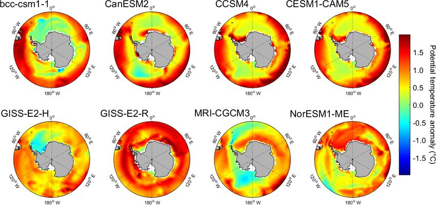
1246                            A. V. Alevropoulos-Borrill et al.: Ocean-forced evolution of the Amundsen Sea catchment

raphy, the depth of the thermocline and the Pacific Ocean         investigated (Bracegirdle et al., 2013; Hosking et al., 2013;
climatology, namely the proximity of the Antarctic Circum-        Little and Urban, 2016; Meijers et al., 2012; Sallée et al.,
polar Current to the continental shelf (Pritchard et al., 2012;   2013a, 2013b), and individual model representation of ob-
Turner et al., 2017). In the ASE, atmospheric and oceanic         served climate varies largely across the ensemble (Flato et
mechanisms drive an upwelling of warm Circumpolar Deep            al., 2013). Comparing the output of AOGCMs against cli-
Water (CDW), reaching up to 4 ◦ C above the in situ melting       matological observations provides a means by which we can
point, which is routed toward the grounding lines of the ASE      investigate biases, assess model performance (Gleckler et al.,
glaciers through dendritic bathymetric troughs (Nakayama et       2008) and identify models that best reproduce observed cli-
al., 2014; Thoma et al., 2008; Turner et al., 2017; Webber et     mate in the Southern Ocean. Assuming performance is tem-
al., 2017). It is widely accepted that CDW is responsible for     porally consistent, projections of climate produced by well-
observed high rates of melting beneath ASE ice shelves (e.g.      performing models can be utilized in experiments establish-
Pritchard et al., 2012; Walker et al., 2013), where periods       ing future basal melt rates (Naughten et al., 2018), thus pro-
of CDW intrusion in the ASE coincide with a speed-up of           viding an input forcing for stand-alone ice sheet models.
glacier velocity (Parizek et al., 2013; Payne, 2007; Shepherd
et al., 2012), making the presence of this water mass on-shelf    2.1   CMIP5 model assessment
an important control on ice dynamics and regional mass loss.
Observations have shown an increase in the quantity of CDW        To identify the CMIP5 models that best reproduce Southern
on-shelf in the ASE (Schmidtko et al., 2014), and projections     Ocean climate, we use the root-mean-square error (RMSE)
show that this will continue in the future, with the increased    performance metric, which is common practice in model
positive phase of the Southern Annular Mode and subsequent        evaluation (Gleckler et al., 2008; Little and Urban, 2016;
strengthening of circumpolar westerlies acting to drive CDW       Naughten et al., 2018). We compare modelled monthly
on-shelf (Bracegirdle et al., 2013; Spence et al., 2014).         CMIP5 output of ocean potential temperature below 30◦ S
   In this investigation, we first identify a subset of Cou-      from January 1979 to December 2016 against the Hadley
pled Model Intercomparison Project Phase 5 (CMIP5)                Centre EN4.2.1 dataset of monthly ocean potential tem-
atmosphere–ocean general circulation models (AOGCMs)              perature (Good et al., 2013; downloaded 8 February 2018)
that best reproduce historical observations of Southern           over the equivalent period. The observational data are cor-
Ocean temperature. Using this subset, we then use the             rected for biases, following the methods of Gouretski and Re-
RCP8.5 projections of ocean temperature anomalies in the          seghetti (2010), and quality control flags are used to nullify
ASE from 2017 to 2100 to parameterize a melt rate forc-           potentially unreliable observations from the dataset. Mod-
ing for the BISICLES ice sheet model. The use of sepa-            els are evaluated over the whole Southern Ocean on the ba-
rate projections from individual AOGCMs provides an in-           sis that teleconnections across the Pacific Ocean have been
dication as to the range of uncertainty associated with the       shown to directly influence ocean heat transport in the ASE
choice of modelled ocean temperature projection and thus          (Steig et al., 2012). Furthermore, there are limited observa-
uncertainty associated with the applied ocean forcing. Fi-        tions in the ASE (Mallett et al., 2018), limiting the validity
nally, we explore the uncertainty associated with the model       of regional evaluation.
initialization procedure through additional experiments with         Given that the historical period defined by the CMIP5 en-
perturbed sets of the spatially varying parameter fields ob-      semble ends in December 2005, we use ocean potential tem-
tained in the initialization procedure. The findings provide      perature projections forced with both RCP2.6 and RCP8.5
fresh insight into the projected migration of the grounding       to make up the remaining decade, from January 2006 to De-
lines of the ASE ice streams when represented by a model          cember 2016, of the observational period. This restricts anal-
with an adapting fine grid resolution adjacent to the ground-     ysis to the 27 AOGCMs with projections for both RCP2.6
ing line. Additionally, we present new constrained estimates      and RCP8.5 scenarios. Given the differences in model resolu-
of the projected sea level contribution from the ASE in re-       tion and depth levels, we perform bilinear interpolation of the
sponse to CMIP5-projected regional ocean forcing under the        gridded model output onto the location of the observational
RCP8.5 “business-as-usual” scenario.                              dataset and further depth-wise linear interpolation, giving the
                                                                  modelled equivalent of each in situ temperature profile. We
                                                                  calculate two separate RMSE scores for each model, using
2   CMIP5 subset                                                  both RCP2.6 and RCP8.5, which we average to give an over-
                                                                  all RMSE for each CMIP5 AOGCM.
The CMIP5 ensemble consists of 50 AOGCMs and Earth
system models (ESMs) from 21 modelling groups (Taylor             2.2   Subset selection
et al., 2012), providing a valuable resource for exploring the
projected future evolution of the climate under varying fu-       Based on the mean RMSE for both RCP2.6 and RCP8.5 sim-
ture emission scenarios. Biases in the representation of cli-     ulations of ocean temperature in the Southern Ocean, we se-
matological features in the Southern Ocean have been widely       lect the six AOGCMs with the lowest score and thus the

The Cryosphere, 14, 1245–1258, 2020                                                   www.the-cryosphere.net/14/1245/2020/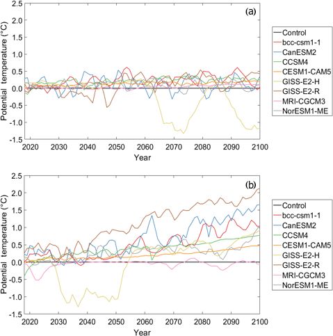
A. V. Alevropoulos-Borrill et al.: Ocean-forced evolution of the Amundsen Sea catchment                                    1247

most realistic representations of observed ocean potential
temperature in the Southern Ocean. The models bcc-csm1-
1, CanESM2, CCSM4, CESM1-CAM5, MRI-CGCM3 and
NorESM1-ME comprise our subset. Additionally, we include
the two additional models in the subset that have the highest
(GISS-E2-R) and lowest (GISS-E2-H) mean projected tem-
perature anomalies over the 21st century, local to the ASE
(see below for zonal calculation), in order to capture the full
range of projected temperatures on-shelf in the ASE across
the CMIP5 ensemble.

2.3   Ocean temperature in the ASE                                Figure 1. Monthly mean ocean potential temperature in the ASE
                                                                  averaged over 400–700 m depth range, produced by a subset of
                                                                  CMIP5 AOGCMs over the period from 1979 to 2016, where the
We explore modelled and observed ocean temperature in the
                                                                  period from 2006 to 2016 is made up of projections forced with
ASE by averaging ocean temperature over the 400–700 m             RCP8.5. Black + symbols show observed ocean potential temper-
layer and then averaging from 103–113◦ W and 72–74◦ S to          ature in the ASE from the Hadley Centre dataset, averaged over
cover the ASE continental shelf. Depths of 400–700 m are          400–700 m depths during the same period.
chosen to represent the depth of CDW on-shelf (Arneborg et
al., 2012; Little and Urban, 2016; Nakayama et al., 2014;
Thoma et al., 2008; Webber et al., 2017). Of the models
that best reproduce temperature over the Southern Ocean,
the range in modelled temperature on-shelf in the ASE is
∼ 2 ◦ C (Fig. 1). Whilst no model is able to capture the range
of observed variability in ocean temperature on-shelf, which
has been shown to oscillate by up to 2 ◦ C (Jenkins et al.,
2018), the collective model output captures the overall range
in observed ocean temperature. Of the CMIP5 models in the
subset, bcc-csm1-1, CanESM2, CCSM4 and NorESM1-ME
most closely reproduce observations on-shelf in the ASE.
Analysis is, however, limited by the number of observations
in the region due to the seasonal dependence of ship access
and lack of mooring-based observations (Kimura et al., 2017)
meaning that seasonal variability is not fully captured by ob-
servations in this (or other) datasets (Mallett et al., 2018).
As no single model captures the observed ocean tempera-
ture variability on-shelf, we argue that the use of a subset,
as opposed to an individual model forcing, is advantageous
as it covers a greater range of possible ocean temperatures
on-shelf.

2.4   CMIP5 ocean temperature projections                         Figure 2. Projected 21st century ASE ocean potential tempera-
                                                                  ture anomalies averaged over 400–700 m depth range. Anomalies
Having identified a subset of AOGCMs, we explore the 21st         are relative to the depth averaged 400–700 m mean from 2005 to
century ocean temperature projections in the ASE as mod-          2016. Each line represents a member of the CMIP5 AOGCM sub-
                                                                  set forced with the RCP8.5 (a) and RCP2.6 (b) scenarios.
elled by each subset member. To gain uniformity of AOGCM
resolution, the projection data from each CMIP5 subset
member is bilinearly interpolated onto a uniform 1◦ ×1◦ hor-
izontal grid. To prescribe a mean ocean temperature forc-         shelf would reside as no ice shelf cavity is represented in the
ing for our ice sheet model experiments, we calculate the         CMIP5 ensemble (Naughten et al., 2018). Whilst projected
mean annual ocean potential temperature anomalies in the          ocean temperatures under the RCP2.6 scenario have been ob-
ASE (Fig. 2). Anomalies are calculated relative to the 2006–      tained, the projected anomalies lie within the range of ocean
2016 temporally averaged mean for the ASE over the 400–           temperature projections for the RCP8.5 scenario. As this in-
700 m depth-averaged layer. The ASE is again defined as           vestigation is interested in exploring a range of temperatures,
the region between 103–113◦ W and 72–74◦ S; a southern            RCP8.5 projections alone have been used in the remainder of
limit is established in order to remove regions where an ice      the study.

www.the-cryosphere.net/14/1245/2020/                                                   The Cryosphere, 14, 1245–1258, 2020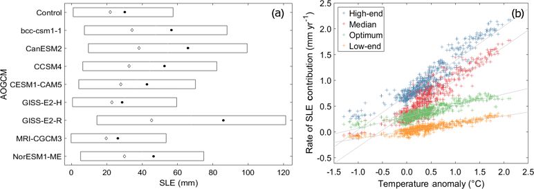
1248                             A. V. Alevropoulos-Borrill et al.: Ocean-forced evolution of the Amundsen Sea catchment

    The modelled range of ocean temperature anomalies un-           3     BISICLES configuration and CMIP5-forced
der the RCP8.5 scenario diverge over the 21st century, with               experiments
a 2.2 ◦ C range in anomalies by 2100. With the exception
of MRI-CGCM3, all models project a temperature increase             3.1    Model description and equations
over the 21st century, relative to the 2006–2016 mean, in
response to the business-as-usual scenario. Ocean warming           To explore the evolution of the ASE in response to CMIP5-
captured by the subset is broadly consistent with the 0.66 ◦ C      forced sub-ice-shelf melt, we use the BISICLES ice flow
full CMIP5 ensemble mean warming over the 21st century in           model. BISICLES is based on the vertically integrated flow
the ASE (Little and Urban, 2016). The models projecting the         model by Schoof and Hindmarsh (2010), which includes lon-
largest increase in temperature over the 21st century, namely       gitudinal and lateral stresses, in addition to a simplification of
GISS-E2-R, CanESM2 and bcc-csm1-1, underestimate ob-                vertical shear stress that is better applied to ice shelves and
served temperature in the ASE during the observational pe-          streams (Cornford et al., 2013; Schoof, 2010). It uses adap-
riod (Fig. 1). Further, the models with warm biases over            tive mesh refinement (AMR) to provide fine resolution near
the observational period, MRI-CGCM3, CESM1-CAM5 and                 the grounding line and a coarser resolution elsewhere. For
GISS-E2-H, project the lowest temperature change over the           the simulations performed in this study, we use five resolu-
projection period.                                                  tion levels with mesh grid spacing of 1x l = 2−l × 4000 m,
    We attribute the projected temperature changes to mod-          where l is an integer between 0 and 4, giving a finest resolu-
elled changes in the quantity of CDW on-shelf in the ASE            tion of 250 m at the grounding line.
(Fig. 3). The behaviour of the models can be characterized             Applying mass conservation to ice thickness and horizon-
by the pattern of temperature change in the Pacific sector of       tal velocity u gives the following equation:
the Southern Ocean, where models display either a localized         ∂h
warming of over 1 ◦ C in the ASE or a regional warming of              + ∇ · (uh) = Ms − Mb ,                                     (1)
                                                                    ∂t
a lower magnitude below 0.5 ◦ C. Models exhibiting local in-
creases in temperature in the ASE over the projection period        where Ms denotes surface mass balance and Mb is the basal
have broadly captured on-shelf temperature over the obser-          melt rate, which, when discretized, is applied solely to cells
vational period (Fig. 1): these are, most notably, bcc-csm1-1,      in which ice is floating.
CanESM2, CCSM4 and NorESM1-ME. We infer the pro-                       Upper-surface elevation s is dependent on ice thickness h
jected localized warming over the 21st century to be a result       and bedrock elevation b, given that ice is assumed to be in
of increased incursion of the CDW layer on-shelf in the ASE.        hydrostatic equilibrium:
Increased CDW presence in the ASE has been observed over
                                                                                             ρi

the last 3 decades (Schmidtko et al., 2014), a trend that is ex-    s = max h + b, 1 −           h ,                           (2)
                                                                                            ρw
pected to continue in the 21st century as a result of a strength-
ening of the circumpolar westerlies that are responsible for        where ρi and ρw describe the respective densities of ice
delivering warm CDW towards the ASE continental shelf               and water.
(Bracegirdle et al., 2013; Gille, 2002; Meijers et al., 2012;          A two-dimensional stress balance equation is also applied,
Sallée et al., 2013b; Spence et al., 2014).                         where the vertically integrated effective viscosity ϕ̇µ is ob-
    In contrast, the models that overestimate temperatures over     tained from both the stiffening factor ϕ and a vertically vary-
the observational period, namely CESM1-CAM5, GISS-E2-               ing effective viscosity µ, which was derived from Glen’s flow
H and MRI-CGCM3, do not display localized future warm-              law. The stress balance equation is therefore formulated as
ing in the ASE, instead showing a muted regional warming.           follows:
We hypothesize two possible explanations for this overes-
timation of observed temperature: either through a modelled         ∇ · [ϕhµ (2ε̇ +2tr (ε̇) I)] + τb = ρi gh∇s,                   (3)
presence of a warm CDW layer on-shelf that does not change          in which the horizontal strain rate tensor is described by the
in depth over the course of the projection period, resulting in     following equation:
little to no change in mean ocean temperature, or a lack of
representation of the CDW incursion mechanism that there-                1h             i
                                                                    ε̇ =    ∇u + (∇u)T .                                       (4)
fore precludes additional modelled upwelling or incursion.               2
                                                                    The vertically varying effective viscosity µ includes repre-
                                                                    sentation of vertical shear strains and, given that the flow rate
                                                                    exponent n = 3, satisfies the following equation:

                                                                    2µA(T ) 4µ2 ε̇2 + |ρi g(s − z)∇s|2 = 1,                       (5)

                                                                    where the temperature-rate-dependent factor A (T ) is calcu-
                                                                    lated using the formula described by Cuffey and Paterson

The Cryosphere, 14, 1245–1258, 2020                                                      www.the-cryosphere.net/14/1245/2020/
A. V. Alevropoulos-Borrill et al.: Ocean-forced evolution of the Amundsen Sea catchment 1249
Figure 3. Projected Southern Ocean temperature anomalies in 2100 (2091–2100 mean), averaged over 400–700 m depth range, under RCP8.5
relative to the 2006–2016 mean for each of the CMIP5 AOGCM subset members.
(2010). Uncertainty in both temperature T and A (T ) is ad- from Rignot et al. (2011). Here we use the ice thickness
dressed by ϕ. The basal traction coefficient C is assumed to (h) and a modified bed topography (b) developed by Nias et
satisfy a non-linear power law, where m = 1/3: al. (2016), which was found by modifying BedMap2 using
an iterative procedure to smooth inconsistencies in the mod-
ρ
−C|u|m−1 u h ρwi > b
τb = . (6) elled flux divergence. The initial sub-shelf melt rate (Mb ) is
0, otherwise also calculated through this iterative procedure (Nias et al.,
2016) to ensure the melt rate at the beginning of the simula-
The initial and applied basal melt rate is parameterized so tion is consistent with present day observations and matches
that it is spatially varying with melt concentrated closest to observed thinning at the grounding line. Further, the model
the grounding line according to the following equation: has been run with a calving front fixed at its initial position.
(
MG (x, y) p (x, y, t) + MA (x, y) floating
Mb (x, y, t) = (1 − p (x, y, t)) , , (7) 3.3 CMIP5 melt rate forcing
0, grounded
We convert the CMIP5 projections of ocean temperature into
where p (x, y, t) = 1 at the grounding line, which then de- a mean additional ocean sub-shelf melt forcing using the lin-
cays exponentially with increasing distance from the ground- ear relationship between temperature anomaly and ice shelf
ing line: melting, which is approximated for the ASE (Rignot and
Jacobs, 2002), where an additional 0.1 ◦ C temperature in-
1, grounded
p − λ2 ∇ 2 p = , (8) crease results in an increase of 1 m a−1 to the basal melt
0, elsewhere
rate. The CMIP5 AOGCM forcing data that we use are rela-
with ∇p · n = 0 as a boundary condition. tively coarse in their spatial resolution and also do not cap-
ture sub-ice-shelf oceanographic conditions. Consequently,
3.2 Input data we are unable to accurately incorporate the spatial complex-
ity of ocean temperature variability that exists in the ASE
To solve the equations described above, the BISICLES ice (Turner et al., 2017). Given that our input data better reflect
sheet model requires numerous input data, which we find regional rather than local-scale oceanic changes, we force
from a number of existing studies. Surface elevation (s) our simulations with spatially averaged CMIP5 temperature
and surface mass balance (Ms ) are obtained from Bedmap2 anomalies.
(Fretwell et al., 2013) and we use a 3D temperature field from The additional sub-shelf melt forcing is applied to the
a higher-order model (Pattyn, 2010). The remaining vari- model using a distance decay function with the greatest melt
ables (C, ϕ, h, b and Mb ) are obtained from the results of an rates located at the grounding line to capture some of the spa-
initialization procedure of BISICLES performed by Nias et tial distribution of melt (Payne, 2007). We use a grounding
al. (2016). Of these parameters, the basal traction coefficient line proximity parameter p as a multiplier, where p = 1 at the
(C) and viscosity stiffening factor (ϕ) are found by solving grounding line and decays exponentially with increasing dis-
an optimization problem, which minimizes the mismatch be- tance. In the 1D case, p (x) = exp(−x/λ), where λ is a scale
tween modelled ice surface speed and the observed speed of 10 000 m. The mean additional forcing is applied onto a
www.the-cryosphere.net/14/1245/2020/ The Cryosphere, 14, 1245–1258, 20201250 A. V. Alevropoulos-Borrill et al.: Ocean-forced evolution of the Amundsen Sea catchment
2D spatially varying field, smoothed to match the pattern of lations with the non-linear sliding law and modified bedrock.
melt obtained during the model initialization procedure. For each parameter set, we perform simulations forced with
The simplified distance-dependent melt parameterization the CMIP5 ocean temperature projections parameterized as a
employed in this investigation was chosen in order to main- sub-ice-shelf melt rate. We present the scaling factors for the
tain continuity with the Nias et al., (2016, 2019) studies. Our four parameter sets used in this investigation (Table 1). The
parameterization neglects the effect of overturning circula- scaling factors describe the level of perturbation for each of
tion within an ice shelf cavity in addition to the ice shelf the spatially varying parameter fields within each of the four
cavity geometry and presence of meltwater plumes that in- parameter sets where a halving is 0, the optimum is 0.5 and
fluence the pattern of sub-ice-shelf basal melting (Dinni- a doubling is 1. When discussing the outcome of the results,
man et al., 2016). Whilst more complex parameterizations we will use these values as a relative comparison.
attempt to incorporate these mechanisms (e.g. Lazeroms et
al., 2018; Reese et al., 2018), no parameterization is yet able 3.5 Experimental design
to replicate known patterns of sub-ice-shelf melting (Favier
et al., 2019). Furthermore, the uncertainty associated with We perform regional simulations of the ASE sector on the
the magnitude of the future forcing exceeds that associated domain defined in Cornford et al. (2015). For each of the
with the parameterization of sub-shelf melting (Holland et four different parameter sets, we use parameterized sub-ice-
al., 2019), justifying the use of the simplified parameteriza- shelf melt rates for each of the eight CMIP5 subset members.
tion employed in this investigation. An additional control experiment is performed for each of the
four parameter sets. The control experiment has no additional
3.4 Parameter selection melt forcing, and therefore the results capture the dynamical
ice response to present conditions. A total of 36 experiments
We investigate the impact of parameter uncertainty on the re- are performed. The following results section firstly describes
sponse of the ASE to the CMIP5 ocean forcing by selecting the results from the optimum parameter set, followed by the
members of a perturbed parameter ensemble performed by results of the experiments using the three perturbed parame-
Nias et al. (2016), which hereafter we will refer to as the N16 ter sets.
ensemble. Here we will briefly describe the N16 ensemble, For our simulations of future mass evolution of the ASE in
before explaining our selection process. As described above, response to changing ocean temperature forcing, we choose
the initialization procedure performed by Nias et al. (2016) to keep the atmospheric forcing constant due to the small
produces three optimal, spatially varying fields of the un- effect of surface mass balance changes on ice stream dynam-
known parameters of basal traction coefficient C, ice stiff- ics (Seroussi et al., 2014), particularly on the timescales we
ening factor ϕ and initial basal melting Mb over the ASE explore in this investigation. Furthermore, ocean-forced sub-
catchment. The N16 ensemble explores the influence of un- shelf melting elicits an immediate response to the upstream
certainty in these parameters on the modelled mass evolution ice dynamics (Seroussi et al., 2014) making this the focus of
and grounding line migration in the ASE by scaling the op- our work.
timal parameter fields between a halving and a doubling and
proceeding to sample these scaled fields using a Latin hyper- 4 Results
cube. The resulting unique combinations of scaled parame-
ters are referred to in this investigation as parameter sets. For 4.1 Optimum parameter set
each perturbed parameter set, a 50-year BISICLES simula-
tion was performed and the change in volume above floata- Our projections show that by the end of the 21st century the
tion (VAF) was used to calculate a sea level equivalent (SLE) CMIP5-forced sub-ice-shelf melting in the ASE will lead to
contribution. This was done for each combination of two ge- a contribution to global mean sea level of 2.0–4.5 cm un-
ometries (modified and unmodified Bedmap2) and two slid- der the RCP8.5 scenario. The range in SLE in response to
ing laws, giving a total of 284 simulations. each CMIP5 sub-ice-shelf melt rate reflects the magnitude
In order to explore the role of parameter uncertainty in of the applied forcing (Fig. 4), where the experiments forced
our study, we select three sets of perturbed parameter fields with CMIP5 models that project the most extreme temper-
from the N16 ensemble, in addition to the optimum. To rep- ature change result in the greatest overall mass contribution
resent a crude 90 % confidence from the variation in param- over the 21st century. The variation in response according
eters, we select the parameter combinations that generated a to AOGCM forcing indicates a strong dependence of ASE
high-end, median and low-end SLE contribution over a 50- mass loss on sub-shelf melting, consistent with existing lit-
year transient experiment in the absence of additional forc- erature (Gudmundsson et al., 2019; Pritchard et al., 2012).
ing. We identify the parameter sets that most closely produce The most extreme response is a result of the GISS-E2-R pro-
the 5th and 95th percentile of a calibrated probability den- jected ocean melting in the ASE, which results in 4.5 cm of
sity function of the N16 ensemble, as described in Nias et sea level rise. The model that projects the lowest-magnitude
al. (2019). In this investigation we solely consider the simu- ocean temperature forcing, MRI-CGCM3, projects a contri-
The Cryosphere, 14, 1245–1258, 2020 www.the-cryosphere.net/14/1245/2020/A. V. Alevropoulos-Borrill et al.: Ocean-forced evolution of the Amundsen Sea catchment 1251
Table 1. Scaling factors applied to each of the spatially varying parameter fields for the parameter sets selected from the N16 ensemble.
Average
Basal Initial rate of SLR over
traction stiffening sub-shelf the 50-year transient
coefficient factor melt rate experiment
(C) (ϕ) (Mb ) (mm yr−1 )
Low-end (B1052) 0.662 0.742 0.730 0.002
Optimum (B0000) 0.500 0.500 0.500 0.269
Median (B1016) 0.856 0.218 0.867 0.316
High-end (B1023) 0.576 0.125 0.884 0.682
infer from the results that, using the optimum parameter set,
grounding line migration over the 21st century is relatively
insensitive to the magnitude of additional forcing, as illus-
trated by the equivalent grounding line positions. The results
from the control experiment denote the projected grounding
line migration should climate conditions remain constant and
therefore reveal the committed sea level contribution from
the ASE in response to current climate.
Across the model subset, the Thwaites Glacier grounding
line is projected to both retreat and lengthen over the 21st
century, with a greater retreat occurring in the eastern side
of the main trunk. A lengthening of the grounding line oc-
curs due to the widening of the ice stream trunk upstream of
Figure 4. Projected 21st century SLE from the ASE in response
the grounding line. In response to the varying forcings, the
to ocean temperature forcing projected by a subset of CMIP5
Thwaites Glacier grounding line experiences approximately
AOGCMS under the RCP8.5 scenario.
the same extent of grounding line migration, which is clus-
tered at points across the main trunk, showing a level of in-
sensitivity to applied forcing. The exception to this ground-
bution of 2.0 cm by 2100, despite having a negligible temper- ing line position is illustrated by the GISS-E2-R-forced ex-
ature change at the end of the 21st century relative to present periment, where migration of the Thwaites Glacier ground-
day. In contrast, the contribution from the control experiment ing line is marginally greater than for the remaining mod-
indicates a committed 2.2 cm contribution to sea level rise els. The relative insensitivity of Thwaites Glacier is consis-
in response to recent past and present day forcing. The SLE tent with previous modelling studies (Tinto and Bell, 2011),
contribution over the projection period is non-linear for mod- which may suggest that the buttressing effect of the uncon-
els with more extreme forcing, which reflects the projected fined ice shelf is minimal and varying magnitudes of sub-
non-linear increase in ocean potential temperature (Fig. 2). shelf melting have a lesser control on the grounding line po-
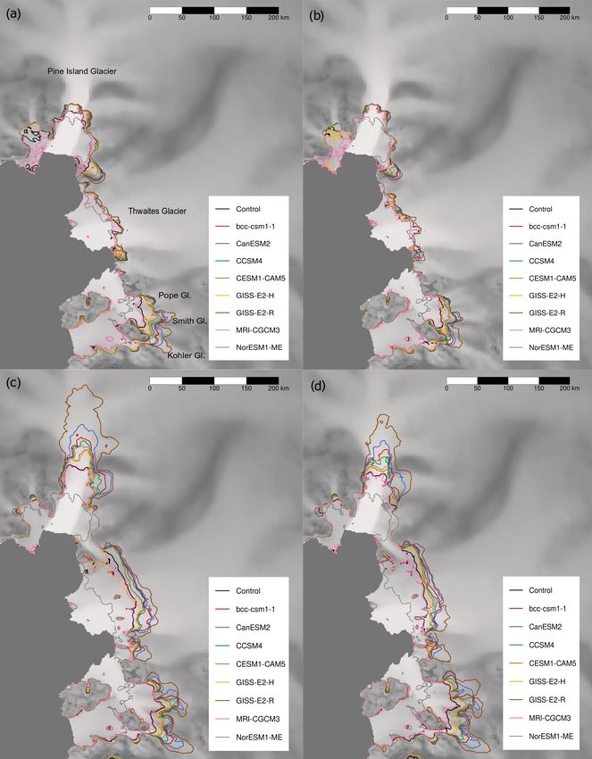
Each of the nine experiments project grounding positions sition (Parizek et al., 2013). Furthermore, retreat to the same
in 2100 retreat relative to the initial grounding line posi- position upstream would indicate that this is a position of
tions (Fig. 5). The response of the individual ice streams to stability, where the grounding line is pinned, likely reflect-
the varying ocean melt forcings differs as a result of their ing the presence of a topographic rise. The fact that migra-
varying topographic confinements and differing ice dynam- tion and lengthening of the grounding line occurs even in the
ics (Nias et al., 2016). Despite the differing magnitudes of control experiment demonstrates that grounding line retreat
the CMIP5 model forcings, the PIG grounding line migrates over the 21st century is almost certain.
25 km upstream from its initial position for all experiments Grounding line retreat of the Pope, Smith and Kohler
except MRI-CGCM3 and the control experiment wherein re- (PSK) ice streams is dependent on the magnitude of the
treat is 11 km, likely controlled by the steep deepening of CMIP5 sub-ice-shelf melt forcing applied. The most extreme
the bed over the initial 10 km upstream of the initial ground- forcing, the GISS-E2-R-forced experiment, results in almost
ing line (Vaughan et al., 2006). Stabilization of the ground- complete loss of grounded area of the small ice streams by
ing line 25 km upstream of its initial location is indicative the end of the 21st century, whilst the control experiment re-
of local topographic maxima at this position (Vaughan et al., sults in grounding line retreat of only ∼ 20 km. The variation
2006) and substantial prograde slope evident in the modi- in grounding line positions in 2100 indicates that the PSK
fied Bedmap2 topography described in the N16 study. We
www.the-cryosphere.net/14/1245/2020/ The Cryosphere, 14, 1245–1258, 20201252 A. V. Alevropoulos-Borrill et al.: Ocean-forced evolution of the Amundsen Sea catchment
Figure 5. ASE ice stream grounding line position in 2100 in response to each CMIP5-AOGCM-projected ocean temperature forcing under
RCP8.5 for each parameter set: (a) optimum, (b) low end, (c) median, (d) high end. The grey grounding line is the initial position.
ice streams are sensitive to the magnitude of ocean forcing, 4.2 Perturbed parameter sets
due to the buttressing provided by the narrow embayment
of the ice streams and the confined Crosson and Dotson ice
shelves (Konrad et al., 2017). As the ice streams are relatively The range in volume above floatation change from the subset
small compared to their neighbours, almost complete loss of of experiments results in a −0.02–1.4 cm SLE contribution
the present ice streams could occur over the 21st century, for the low-end parameter set, 2.6–8.6 cm for the median pa-
even in the absence of additional ocean forcing (Scheuchl et rameter set and 5.4–12.1 cm for the high-end parameter set.
al., 2016). As illustrated by the differing range of SLE contributions
across the four parameter sets, the sensitivity of the ASE to
different additional sub-shelf melt forcings varies with differ-
ing spatially varying parameter fields. Again, the magnitude
The Cryosphere, 14, 1245–1258, 2020 www.the-cryosphere.net/14/1245/2020/A. V. Alevropoulos-Borrill et al.: Ocean-forced evolution of the Amundsen Sea catchment 1253 of mass loss is proportional to the magnitude of the applied ing across the wide glacier trunk for each of the CMIP5- forcing for each of the CMIP5-forced experiments, and this forced experiments, in addition to an upstream retreat where relationship is consistent across the three perturbed parame- the widening of the embayment has a greater control on the ter sets. mass flux from the ice stream. For all parameter sets, the PSK Experiments configured with the low-end parameter set re- ice streams exhibit notable grounding line retreat, controlled sult in the most modest grounding line retreat across the ASE largely by the varying magnitudes of applied ocean forcing. ice streams (Fig. 5). The PIG grounding line is projected to There is a significant correlation between the rate of SLE retreat ∼ 14 km upstream of the main trunk for each of the contribution and the applied CMIP5 ocean anomaly, with an CMIP5-forced experiments, with retreat into the southwest- R 2 value of > 0.9, which is consistent for each of the param- ern tributary occurring in some scenarios in response to the eter sets (Fig. 6b). Whilst the response of the ASE ice streams different forcing magnitudes. The projected grounding line to ocean temperature forcing is linear for each parameter set, position of Thwaites Glacier by the end of the 21st cen- the sensitivity to forcing is dependent on the parameter set tury for the low-end parameter set is most equivalent to the chosen in the ice sheet model configuration, modifying both present day position, experiencing minimal retreat with only the gradient and intercept of the SLE response to temperature minor variation between the different CMIP5-forced experi- forcing. Moreover, the uncertainty associated with the pro- ments. Of the ASE ice streams, the Thwaites Glacier ground- jected SLE contribution for each AOGCM is dependent on ing line position varies most in comparison to the optimum. the parameter set (Fig. 6b), where models with the greatest Similar to the optimum parameter set experiments, the PSK ocean temperature forcing result in the largest range in SLE grounding line retreat differs considerably in response to the contribution when accounting for the parameter uncertainty. varying CMIP5 forcings, with the greatest retreat occurring in response to the GISS-E2-R forcing. Overall, the ground- ing line positions under the low-end parameter configuration 5 Discussion are similar to the optimum. Mass loss and grounding line re- treat is limited under this configuration due to the increased For the optimum set of parameters obtained in the initializa- stiffness and greater basal traction, limiting delivery of ice to tion procedure, we project a 2.0–4.5 cm SLE contribution in the grounding line and subsequent mass loss. response to CMIP5 RCP8.5 projections of ocean tempera- In comparison to the low-end and optimum parameter sets, ture on-shelf in the ASE. The greater the magnitude of the the median and high-end parameter sets produce consider- temperature anomaly over the 21st century, the more exten- able grounding line retreat in response to each of the CMIP5- sive the grounding line retreat and projected mass loss from projected sub-ice-shelf melt forcings. Both parameter sets the ASE, which is consistent with findings from modelling have a similarly low scaling of the ice viscosity and a high studies and observations (Favier et al., 2014). Recent lit- initial basal melt rate in comparison to the optimum, which is erature has established a close coupling between the basal likely responsible for the greater mass loss (Nias et al., 2016). melting of ice shelves and exacerbated grounding line retreat The median set of parameters results in a greater grounding (Arthern and Williams, 2017; Christianson et al., 2016; Glad- line retreat over the 21st century than the high-end parameter stone et al., 2012; Pritchard et al., 2012; Ritz et al., 2015; set, despite the lower overall mass loss. This occurs because Seroussi et al., 2014). Given that our applied sub-shelf melt the high-end parameter set has a lower scaling factor applied rates are derived from CMIP5 modelled ocean temperature to the basal traction coefficient field than the median set, pro- projections, it is evident that models displaying the greatest ducing a more slippery bed in the former than the latter, caus- magnitude of local warming in the ASE produce the greatest ing increased delivery of mass toward the grounding line and grounding line retreat and SLE by the end of the 21st cen- offsetting grounding line retreat. Combined with softer ice tury (Jacobs et al., 2012; Turner et al., 2017; Wåhlin et al., and increased velocity, the relatively slippery bed also results 2013), where large warming is likely associated with an in- in increased delivery of mass across the grounding line, ex- creased volume of CDW on-shelf (Thoma et al., 2008). The plaining the high projected mass loss and SLE contribution varying responses to the different AOGCM forcings illustrate of between 5.4 and 12.1 cm by 2100, despite the more muted the dependence of the region on the sub-ice-shelf melt forc- grounding line retreat. ing, highlighting the uncertainty in SLE projections resulting The response of the individual ice streams to additional from choice of AOGCM alone. melt forcing is similar for the median and high-end parame- Existing modelling investigations exploring future ASE ter sets. The PIG grounding line retreat is predominantly con- mass evolution indicate a range of SLE contributions by fined to its narrow embayment with considerable upstream the end of the 21st century, due to the differences in model retreat into the main trunk. For both parameter sets, the PIG physics and experimental design. Cornford et al. (2015) grounding line is sensitive to the magnitude of the CMIP5 found a 1.5 to 4.0 cm SLE in response to the A1B scenario ocean temperature forcing, with large differences between from CMIP3, which is consistent with our findings, despite the final positions in 2100 across the subset. The Thwaites the A1B scenario being of a lower-magnitude forcing than Glacier grounding line experiences a considerable lengthen- RCP8.5. Furthermore, a 16-member ice sheet model inter- www.the-cryosphere.net/14/1245/2020/ The Cryosphere, 14, 1245–1258, 2020
1254                              A. V. Alevropoulos-Borrill et al.: Ocean-forced evolution of the Amundsen Sea catchment

Figure 6. (a) Sea level equivalent contribution from the ASE in 2100 for each AOGCM in the subset under the RCP8.5 scenario for the range
of parameter sets. The top and tail of the boxes show the high- and low-end perturbed parameter sets, respectively. The diamond and circle
show the SLE contribution for the optimum and median parameter sets, respectively. (b) Rate of SLE response against ocean temperature
anomaly in the ASE, averaged over the 400–700 m layer, over the projection period from 2017 to 2100 for each set of parameters.

comparison study projecting the response to an RCP8.5 sce-             by the results of the full N16 ensemble. However, the re-
nario by Levermann et al. (2020) gave a 90 % likelihood                sponse of the region to the perturbed basal traction param-
upper-bound SLE contribution of approximately 9 cm rela-               eters is not consistent with the expected trend that has been
tive to the year 2000, with a median of 2 cm. Whilst the               illustrated through linear regression (Nias et al., 2016), in-
uncertainty range in their investigation is derived from the           stead perturbed parameters increase in the order of optimum,
differences between the ice sheet models, and thus their res-          high end, low end and median, while the mass loss increases
olutions and model physics, the study does not account for             from low to high. This relationship may arise partly because
uncertainty associated with individual model configuration,            our experiments explore only a sample of the theoretical pa-
which would result in a greater uncertainty range in SLE pro-          rameter space, whereas other, unmodelled, parameter combi-
jections. Our projected 21st century sea level rise estimates          nations might show clearer dependencies. However, the lack
are broadly consistent with existing investigations despite the        of linearity between basal traction and mass loss may also
use of alternative forcing scenarios and models.                       indicate that the latter is more strongly influenced by varia-
   The relationship between the applied sub-ice-shelf melt             tions in, for example, ice viscosity, than by basal friction. The
forcing and the rate of SLE response suggests that the ASE             range of SLE projections in response to varied ocean forcing
is responding linearly to ocean temperature (Fig. 6b); this is         is therefore dependent on the specific combination of these
consistent across the low-end, optimum, median and high-               individual spatially varying parameters, and, in our experi-
end parameter sets. The linearity of our results would indi-           ments, the range in SLE uncertainty attributable to parameter
cate that MISI is not observed in the ASE during the 21st              selection exceeds that from choice of AOGCM forcing.
century simulations, where runaway mass loss and ground-                  A notable deficiency with using a stand-alone ice sheet
ing line retreat in the region would exhibit a more non-linear         model lies in the inability of experiments to capture the melt-
SLE contribution. Previous modelling studies have, however,            water feedback (Donat-Magnin et al., 2017). As increased
shown that a MISI response may occur this century under                temperatures result in basal melting, the input of cold fresh
very high melt rate forcing (Arthern and Williams, 2017) or            water alters ocean properties and circulation, resulting in a
in the 22nd century following a perturbation applied during            modification of the ocean forcing of ice shelves (Hellmer et
the 21st century (e.g. Martin et al., 2019). Therefore, our re-        al., 2017). The inclusion of meltwater has been modelled to
sults do not preclude that multi-centennial MISI may have              result in an increased stratification of the water column and
been initiated in the simulations performed in this investiga-         reduction in mixing, meaning the CDW routed toward the
tion.                                                                  grounding line is unmodified, resulting in enhanced melt-
   We find the uncertainty associated with the ice sheet               ing compared with uncoupled ice ocean model experiments
model parameters, C, ϕ and Mb , obtained in the initializa-            (Bronselaer et al., 2018; Golledge et al., 2019). Addition-
tion procedure alters the sensitivity of the ASE response to           ally, the velocity of sub-ice-shelf melt plumes, controlled by
ocean-forced basal melting. The sensitivity of projections             ocean circulation in addition to ice shelf cavity geometry, is
to uncertainties associated with model parameters increases            influential on the sub-shelf melting (Dinniman et al., 2016)
with increasing magnitude of ocean forcing, consistent with            and will be neglected with our simplified ocean temperature
Bulthuis et al. (2019). Generally, increased (decreased) vis-          forcing. Coupling of the ice sheet model to a cavity-resolving
cosity, basal traction and decreased (increased) initial basal         ocean model (e.g. Naughten et al., 2018) would reduce these
melt act to suppress (amplify) the mass loss from the ASE              limitations, though at present this remains computationally
ice streams and projected SLE estimates, which is illustrated          expensive (Cornford et al., 2015), and thus simple ocean-

The Cryosphere, 14, 1245–1258, 2020                                                          www.the-cryosphere.net/14/1245/2020/
A. V. Alevropoulos-Borrill et al.: Ocean-forced evolution of the Amundsen Sea catchment                                              1255

temperature-forced experiments such as ours remain a viable           National Laboratory, California, USA, and Stephen L. Cornford at
approach.                                                             Swansea University.

                                                                      Review statement. This paper was edited by Olaf Eisen and re-
6   Conclusions                                                       viewed by Daniel Martin and one anonymous referee.

In this investigation we use 21st century CMIP5 RCP8.5 pro-
jections of ocean temperature from a historically validated
subset of AOGCMs to parameterize a sub-ice-shelf melt rate            References
forcing for ice streams in the ASE. Using a set of optimum
spatially varying parameters obtained from the model con-             Alevropoulos-Borrill, A.: Ocean forced evolution of
figuration procedure, we find a contribution to sea level rise          the Amundsen Sea catchment by 2100, OSF home,
of 2.0–4.5 cm by 2100, where the SLE response of the ASE                https://doi.org/10.17605/OSF.IO/HQPS7, 2019.
is largely dependent on the choice of AOGCM forcing ap-               Arneborg, L., Wahlin, A. K., Björk, G., Liljebladh, B.,
plied. Additional experiments using perturbed spatially vary-           and Orsi, A. H.: Persistent inflow of warm water onto
ing parameter fields of basal traction, ice stiffness and initial       the central Amundsen shelf, Nat. Geosci., 5, 876–880,
sub-shelf melt rate reveal a 12.1 cm upper-bound SLE contri-            https://doi.org/10.1038/ngeo1644, 2012.
bution for a crude 90 % uncertainty associated with the con-          Arthern, R. J. and Williams, C. R.: The sensitivity of West Antarc-
                                                                        tica to the submarine melting feedback, Geophys. Res. Lett., 44,
figuration procedure. We find the response of the region, as
                                                                        2352–2359, https://doi.org/10.1002/2017GL072514, 2017.
shown by the projected mass loss, to be dependent largely             Bracegirdle, T. J., Shuckburgh, E., Sallee, J. B., Wang, Z., Meijers,
on the magnitude of applied forcing, which has been derived             A. J. S., Bruneau, N., Phillips, T., and Wilcox, L. J.: Assessment
from projections of ocean temperature in the region. We take            of surface winds over the atlantic, indian, and pacific ocean sec-
forward from this investigation that the perturbation of ice            tors of the southern ocean in cmip5 models: Historical bias, forc-
sheet model parameter fields has a considerable control on              ing response, and state dependence, J. Geophys. Res.-Atmos.,
the projected response of the region to ocean-forced basal              118, 547–562, https://doi.org/10.1002/jgrd.50153, 2013.
melting, highlighting the importance of reducing uncertainty          Bronselaer, B., Stouffer, R. J., Winton, M., Griffies, S. M., Hurlin,
associated with ice sheet model initialization and parameter            W. J., Russell, J. L., Rodgers, K. B., and Sergienko, O. V.:
choice.                                                                 Change in future climate due to Antarctic meltwater, Nature, 564,
                                                                        53–58, https://doi.org/10.1038/s41586-018-0712-z, 2018.
                                                                      Bulthuis, K., Arnst, M., Sun, S., and Pattyn, F.: Uncertainty
                                                                        quantification of the multi-centennial response of the Antarctic
Data availability. CMIP5 output can be obtained from
                                                                        ice sheet to climate change, The Cryosphere, 13, 1349–1380,
http://esgf-node.llnl.gov (last access: May 2018; Lawrence
                                                                        https://doi.org/10.5194/tc-13-1349-2019, 2019.
Livermore National Laboratory, 2020). The EN4.2.1. dataset
                                                                      Christianson, K., Bushuk, M., Dutrieux, P., Parizek, B. R., Joughin,
can be obtained from https://www.metoffice.gov.uk/hadobs/en4/
                                                                        I. R., Alley, R. B., Shean, D. E., Abrahamsen, E. P., Anandakr-
(last access: May 2018; Met Office, 2020). Data support-
                                                                        ishnan, S., Heywood, K. J., Kim, T. W., Lee, S. H., Nicholls, K.,
ing the main conclusions of this study can be found at
                                                                        Stanton, T., Truffer, M., Webber, B. G. M., Jenkins, A., Jacobs,
https://doi.org/10.17605/OSF.IO/HQPS7    (Alevropoulos-Borrill,
                                                                        S., Bindschadler, R., and Holland, D. M.: Sensitivity of Pine Is-
2019). For the BISICLES ice sheet model spatial data in hdf5
                                                                        land Glacier to observed ocean forcing, Geophys. Res. Lett., 43,
format, please contact the lead author.
                                                                        10817–10825, https://doi.org/10.1002/2016GL070500, 2016.
                                                                      Church, J. A., Gregory, J. M., Cazenave, A., Gregory, J. M.,
                                                                        Jevrejeva, S., Levermann, A., Milne, G. A., Payne, A., Stam-
Author contributions. AVA-B performed the model simulations             mer, D., Box, J. E., Carson, M., Collins, W. R. G., Forster,
and analysis under the guidance of AJP. IJN provided the ice sheet      P., Gardner, A., and Good, P.: IPCC 2014, Ch. 13: Sea Level
model setup, parameter ensemble and support with analysis. RJB          Change, Clim. Chang. 2013 Phys. Sci. Basis. Contrib. Work. Gr.
provided the CMIP5 model output and assisted with ocean data            I to Fifth Assess. Rep. Intergov. Panel Clim. Chang., 639–693,
analysis. The manuscript was written by AVAB with contributions         https://doi.org/10.1017/CBO9781107415324.026, 2013.
from IJN and NRG.                                                     Cornford, S. L., Martin, D. F., Graves, D. T., Ranken, D. F.,
                                                                        Le Brocq, A. M., Gladstone, R. M., Payne, A. J., Ng, E. G.,
                                                                        and Lipscomb, W. H.: Adaptive mesh, finite volume model-
Competing interests. The authors declare that they have no conflict     ing of marine ice sheets, J. Comput. Phys., 232, 529–549,
of interest.                                                            https://doi.org/10.1016/j.jcp.2012.08.037, 2013.
                                                                      Cornford, S. L., Martin, D. F., Payne, A. J., Ng, E. G., Le Brocq, A.
                                                                        M., Gladstone, R. M., Edwards, T. L., Shannon, S. R., Agosta,
Acknowledgements. BISICLES simulations were carried out on the          C., van den Broeke, M. R., Hellmer, H. H., Krinner, G., Ligten-
University of Bristol’s Blue Crystal Phase 3 supercomputer. BISI-       berg, S. R. M., Timmermann, R., and Vaughan, D. G.: Century-
CLES development is led by Daniel F. Martin at Lawrence Berkeley        scale simulations of the response of the West Antarctic Ice

www.the-cryosphere.net/14/1245/2020/                                                         The Cryosphere, 14, 1245–1258, 2020
1256 A. V. Alevropoulos-Borrill et al.: Ocean-forced evolution of the Amundsen Sea catchment Sheet to a warming climate, The Cryosphere, 9, 1579–1600, Golledge, N. R., Keller, E. D., Gomez, N., Naughten, K. A., https://doi.org/10.5194/tc-9-1579-2015, 2015. Bernales, J., Trusel, L. D., and Edwards, T. L.: Global envi- Cuffey, K. M. and Paterson, W. S. B.: The physics of glaciers, Aca- ronmental consequences of twenty-first-century ice-sheet melt, demic Press, 2010. Nature, 566, 65–72, https://doi.org/10.1038/s41586-019-0889-9, Dinniman, M., Asay-Davis, X., Galton-Fenzi, B., Holland, P., Jenk- 2019. ins, A., and Timmermann, R.: Modeling Ice Shelf/Ocean In- Good, S. A., Martin, M. J., and Rayner, N. A.: EN4: teraction in Antarctica: A Review, Oceanography, 29, 144–153, Quality controlled ocean temperature and salinity pro- https://doi.org/10.5670/oceanog.2016.106, 2016. files and monthly objective analyses with uncertainty Donat-Magnin, M., Jourdain, N. C., Spence, P., Le Sommer, J., estimates, J. Geophys. Res.-Ocean., 118, 6704–6716, Gallée, H., and Durand, G.: Ice-Shelf Melt Response to Chang- https://doi.org/10.1002/2013JC009067, 2013. ing Winds and Glacier Dynamics in the Amundsen Sea Sec- Gouretski, V. and Reseghetti, F.: On depth and temperature bi- tor, Antarctica, J. Geophys. Res.-Ocean., 122, 10206–10224, ases in bathythermograph data: Development of a new correction https://doi.org/10.1002/2017JC013059, 2017. scheme based on analysis of a global ocean database, Deep. Res. Favier, L., Durand, G., Cornford, S. L., Gudmundsson, G. H., Pt. I, 57, 812–833, https://doi.org/10.1016/j.dsr.2010.03.011, Gagliardini, O., Gillet-Chaulet, F., Zwinger, T., Payne, A. J., 2010. and Le Brocq, A. M.: Retreat of Pine Island Glacier controlled Gudmundsson, G. H.: Ice-shelf buttressing and the stabil- by marine ice-sheet instability, Nat. Clim. Change, 4, 117–121, ity of marine ice sheets, The Cryosphere, 7, 647–655, https://doi.org/10.1038/nclimate2094, 2014. https://doi.org/10.5194/tc-7-647-2013, 2013. Favier, L., Jourdain, N. C., Jenkins, A., Merino, N., Durand, G., Gudmundsson, G. H., Paolo, F. S., Adusumilli, S., and Fricker, H. Gagliardini, O., Gillet-Chaulet, F., and Mathiot, P.: Assess- A.: Instantaneous Antarctic ice sheet mass loss driven by thin- ment of sub-shelf melting parameterisations using the ocean– ning ice shelves, Geophys. Res. Lett., 46, 13903–13909, 2019. ice-sheet coupled model NEMO(v3.6)–Elmer/Ice(v8.3) , Geosci. Hellmer, H. H., Kauker, F., Timmermann, R., and Hatter- Model Dev., 12, 2255–2283, https://doi.org/10.5194/gmd-12- mann, T.: The fate of the Southern Weddell sea continen- 2255-2019, 2019. tal shelf in a warming climate, J. Climate, 30, 4337–4350, Flato, G., Marotzke, J., Abiodun, B., Braconnot, P., Chou, S. C., https://doi.org/10.1175/JCLI-D-16-0420.1, 2017. Collins, W., Cox, P., Driouech, F., Emori, S., Eyring, V., Forest, Holland, P. R., Bracegirdle, T. J., Dutrieux, P., Jenkins, A., and C., Gleckler, P., Guilyardi, E., Jakob, C., Kattsov, V., Reason, C., Steig, E. J.: West Antarctic ice loss influenced by internal climate and Rummukainen, M.: Chapter 9: Evaluation of Climate Mod- variability and anthropogenic forcing, Nat. Geosci., 12, 718–724, els, Clim. Chang. 2013 Phys. Sci. Basis. Contrib. Work. Gr. I https://doi.org/10.1038/s41561-019-0420-9, 2019. to Fifth Assess. Rep. Intergov. Panel Clim. Change, 741–866, Hosking, J. S., Orr, A., Marshall, G. J., Turner, J., and Phillips, https://doi.org/10.1017/CBO9781107415324, 2013. T.: The influence of the amundsen-bellingshausen seas low on Fretwell, P., Pritchard, H. D., Vaughan, D. G., Bamber, J. L., Bar- the climate of West Antarctica and its representation in cou- rand, N. E., Bell, R., Bianchi, C., Bingham, R. G., Blanken- pled climate model simulations, J. Climate, 26, 6633–6648, ship, D. D., Casassa, G., Catania, G., Callens, D., Conway, H., https://doi.org/10.1175/JCLI-D-12-00813.1, 2013. Cook, A. J., Corr, H. F. J., Damaske, D., Damm, V., Ferracci- Jacobs, S., Jenkins, A., Hellmer, H., Giulivi, C., Nitsche, oli, F., Forsberg, R., Fujita, S., Gim, Y., Gogineni, P., Griggs, F., Huber, B., and Guerrero, R.: The Amundsen Sea J. A., Hindmarsh, R. C. A., Holmlund, P., Holt, J. W., Jacobel, and the Antarctic Ice Sheet, Oceanography, 25, 154–163, R. W., Jenkins, A., Jokat, W., Jordan, T., King, E. C., Kohler, https://doi.org/10.5670/oceanog.2012.90, 2012. J., Krabill, W., Riger-Kusk, M., Langley, K. A., Leitchenkov, Jenkins, A., Shoosmith, D., Dutrieux, P., Jacobs, S., Kim, T. G., Leuschen, C., Luyendyk, B. P., Matsuoka, K., Mouginot, W., Lee, S. H., Ha, H. K., and Stammerjohn, S.: West J., Nitsche, F. O., Nogi, Y., Nost, O. A., Popov, S. V., Rignot, Antarctic Ice Sheet retreat in the Amundsen Sea driven E., Rippin, D. M., Rivera, A., Roberts, J., Ross, N., Siegert, by decadal oceanic variability, Nat. Geosci., 11, 733–738, M. J., Smith, A. M., Steinhage, D., Studinger, M., Sun, B., https://doi.org/10.1038/s41561-018-0207-4, 2018. Tinto, B. K., Welch, B. C., Wilson, D., Young, D. A., Xiangbin, Kimura, S., Jenkins, A., Regan, H., Holland, P. R., Assmann, C., and Zirizzotti, A.: Bedmap2: improved ice bed, surface and K. M., Whitt, D. B., Van Wessem, M., van de Berg, W. thickness datasets for Antarctica, The Cryosphere, 7, 375–393, J., Reijmer, C. H., and Dutrieux, P.: Oceanographic Con- https://doi.org/10.5194/tc-7-375-2013, 2013. trols on the Variability of Ice-Shelf Basal Melting and Cir- Gille, S. T.: Warming of the Southern Ocean since the 1950s, Sci- culation of Glacial Meltwater in the Amundsen Sea Embay- ence, 295, 1275–1277, https://doi.org/10.1126/science.1065863, ment, Antarctica, J. Geophys. Res.-Ocean., 122, 10131–10155, 2002. https://doi.org/10.1002/2017JC012926, 2017. Gladstone, R. M., Lee, V., Rougier, J., Payne, A. J., Hellmer, Konrad, H., Gilbert, L., Cornford, S. L., Payne, A., Hogg, H., Le Brocq, A., Shepherd, A., Edwards, T. L., Gregory, A., Muir, A., and Shepherd, A.: Uneven onset and pace J., and Cornford, S. L.: Calibrated prediction of Pine Island of ice-dynamical imbalance in the Amundsen Sea Embay- Glacier retreat during the 21st and 22nd centuries with a cou- ment, West Antarctica, Geophys. Res. Lett., 44, 910–918, pled flowline model, Earth Planet. Sci. Lett., 333, 191–199, https://doi.org/10.1002/2016GL070733, 2017. https://doi.org/10.1016/j.epsl.2012.04.022, 2012. Lawrence Livermore National Laboratory: Coupled Model Inter- Gleckler, P. J., Taylor, K. E., and Doutriaux, C.: Performance met- comparison Project 5 (CMIP5), available at: https://esgf-node. rics for climate models, J. Geophys. Res.-Atmos., 113, D06104, llnl.gov/projects/esgf-llnl/ (last access: May 2018), 2020. https://doi.org/10.1029/2007JD008972, 2008. The Cryosphere, 14, 1245–1258, 2020 www.the-cryosphere.net/14/1245/2020/
You can also read