Future shifts in extreme flow regimes in Alpine regions - HESS
←
→
Page content transcription
If your browser does not render page correctly, please read the page content below
Hydrol. Earth Syst. Sci., 23, 4471–4489, 2019
https://doi.org/10.5194/hess-23-4471-2019
© Author(s) 2019. This work is distributed under
the Creative Commons Attribution 4.0 License.

Future shifts in extreme flow regimes in Alpine regions
Manuela I. Brunner1 , Daniel Farinotti1,2 , Harry Zekollari1,2,3 , Matthias Huss2,4 , and Massimiliano Zappa1
1 Swiss Federal Institute for Forest, Snow and Landscape Research WSL, Birmensdorf ZH, Switzerland
2 Laboratory of Hydraulics, Hydrology and Glaciology (VAW), ETH Zürich, Zurich, Switzerland
3 Laboratoire de Glaciologie, Université Libre de Bruxelles, Brussels, Belgium
4 Department of Geosciences, University of Fribourg, Fribourg, Switzerland

Correspondence: Manuela I. Brunner (manuela.brunner@wsl.ch)

Received: 2 April 2019 – Discussion started: 9 April 2019
Revised: 18 June 2019 – Accepted: 9 September 2019 – Published: 30 October 2019

Abstract. Extreme low and high flows can have negative             in water resource planning and management and the extreme
economic, social, and ecological effects and are expected          regime estimates are a valuable basis for climate impact
to become more severe in many regions due to climate               studies.
change. Besides low and high flows, the whole flow regime,
i.e., annual hydrograph comprised of monthly mean flows,           Highlights
is subject to changes. Knowledge on future changes in flow
regimes is important since regimes contain information                 1. Estimation of 100-year low- and high-flow regimes us-
on both extremes and conditions prior to the dry and wet                  ing annual flow duration curves and stochastically sim-
seasons. Changes in individual low- and high-flow char-                   ulated discharge time series
acteristics as well as flow regimes under mean conditions              2. Both mean and extreme regimes will change under fu-
have been thoroughly studied. In contrast, little is known                ture climate conditions.
about changes in extreme flow regimes. We here propose
two methods for the estimation of extreme flow regimes                 3. The minimum discharge of extreme regimes will de-
and apply them to simulated discharge time series for future              crease in rainfall-dominated regions but increase in
climate conditions in Switzerland. The first method relies                melt-dominated regions.
on frequency analysis performed on annual flow duration
curves. The second approach performs frequency analysis of             4. The maximum discharge of extreme regimes will in-
the discharge sums of a large set of stochastically generated             crease and decrease in rainfall-dominated and melt-
annual hydrographs. Both approaches were found to produce                 dominated regions, respectively.
similar 100-year regime estimates when applied to a data set
of 19 hydrological regions in Switzerland. Our results show
that changes in both extreme low- and high-flow regimes
for rainfall-dominated regions are distinct from those in          1    Introduction
melt-dominated regions. In rainfall-dominated regions, the
minimum discharge of low-flow regimes decreases by up to           Low flows can have severe impacts on ecology and econ-
50 %, whilst the reduction is 25 % for high-flow regimes.          omy. Potential ecological impacts include fish-habitat condi-
In contrast, the maximum discharge of low- and high-flow           tions or water quality (Rolls et al., 2012), whilst economi-
regimes increases by up to 50 %. In melt-dominated regions,        cal impacts comprise water supply, river transport, agricul-
the changes point in the other direction than those in rainfall-   ture, and energy production (Van Loon, 2015). The inten-
dominated regions. The minimum and maximum discharges              sity of such potentially harmful low flows is projected to
of extreme regimes increase by up to 100 % and decrease by         increase in the future due to climate change (Alderlieste
less than 50 %, respectively. Our findings provide guidance        et al., 2014; Papadimitriou et al., 2016; Marx et al., 2018).
                                                                   Also, high flows, which can cause severe damages and major

Published by Copernicus Publications on behalf of the European Geosciences Union.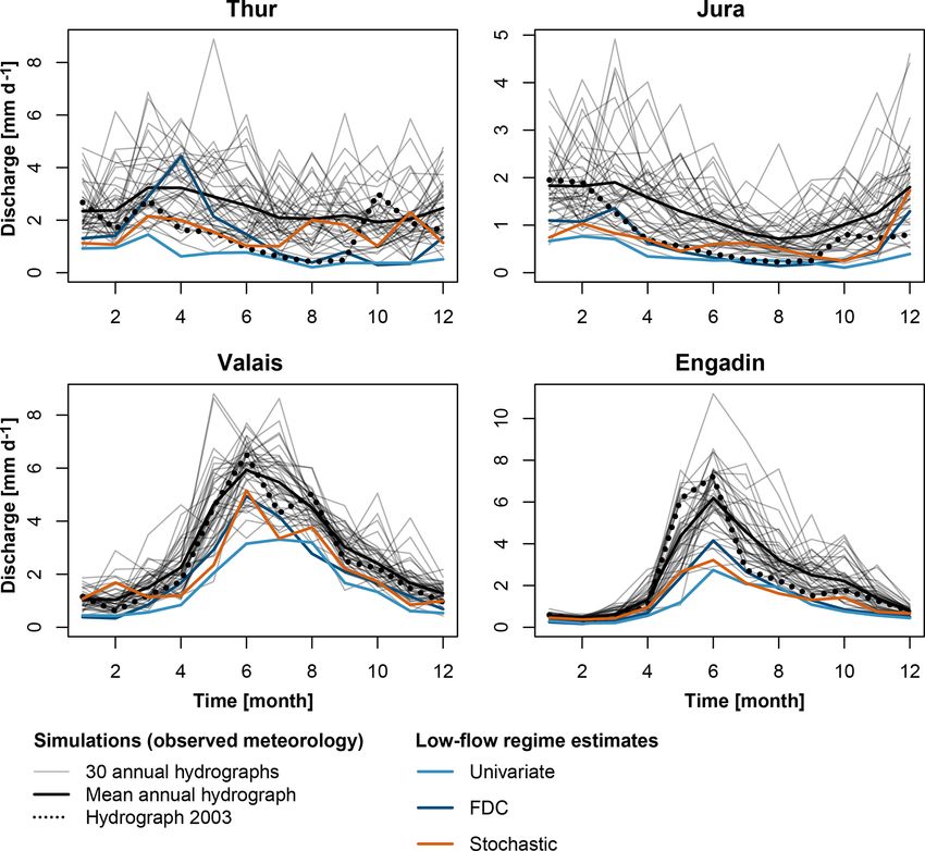
4472                                                       M. I. Brunner et al.: Extreme, current, and future runoff regimes

costs (Aon Benfield, 2016), are expected to change in fu-          timation of such extreme regimes. The first approach is
ture. While clear patterns of change have been detected for        based on flow duration curves (FDCs). FDCs describe the
flood timing (Blöschl et al., 2017), changes in magnitude are      whole distribution of discharge and are particularly suited for
less clear than for low flows (Madsen et al., 2014). Together      planning purposes (Vogel and Fennessey, 1994; Claps and
with low and high flows, the whole flow regime, which de-          Fiorentino, 1997). It has been shown that frequency analy-
picts the magnitude, variability, and seasonality of discharge     sis performed on annual FDCs allows for the estimation of
during the year (Poff et al., 1997), is expected to change (Ar-    extreme FDCs with pre-defined return periods (Castellarin
nell, 1999; Horton et al., 2006; Laghari et al., 2012; Addor       et al., 2004; Iacobellis, 2008). While such estimates contain
et al., 2014; Milano et al., 2015). Such changes are caused by     information on the frequency of occurrence and the distri-
reduced snow and glacier storage (Beniston et al., 2018), re-      bution of flow, they lack information on the seasonality of
lated reductions in melt contributions (Farinotti et al., 2016;    flow (Vogel and Fennessey, 1994). FDC estimates derived
Jenicek et al., 2018), and changes in precipitation seasonal-      for a certain return period T therefore need to be recom-
ity and intensity (Brönnimann et al., 2018). It is important       bined with a specific seasonality, e.g., the long-term one.
to quantify these hydrological changes to adapt water gover-       This first estimation approach treats distribution and season-
nance and management accordingly (Clarvis et al., 2014).           ality separately. To overcome this problem, an alternative ap-
   Previous studies have focused on the detection of changes       proach based on stochastically generated time series is pro-
in mean flow regimes (Horton et al., 2006; Addor et al., 2014;     posed. Stochastically generated time series have been used in
Milano et al., 2015). For planning purposes and river basin        a number of water resource studies, including hydrologic de-
management, however, estimates not only for mean condi-            sign and drought planning (Koutsoyiannis, 2000). Stochas-
tions, but also for extreme conditions, are needed (Van Loon,      tic approaches generate large sets of realizations of possi-
2015; Ternynck et al., 2016). Extreme regime estimates,            ble discharge time series, thus sampling hydrologic vari-
which describe the evolution of flow over the year under ex-       ability beyond the historical record (Herman et al., 2016;
treme conditions, provide guidance for water managers, de-         Tsoukalas et al., 2018), potentially including extreme events
cision makers, and engineers involved in planning and wa-          and regimes. In hydrology, stochastic models have been de-
ter management. They are essential for the adaptation of hy-       veloped so as to reproduce key statistical features of observed
draulic infrastructure such as reservoirs and for developing       data, including the distribution and the temporal dependence
suitable water management and flood protection strategies.         (Sharma et al., 1997; Salas and Lee, 2010; Tsoukalas et al.,
   Commonly, extreme flow estimates derived by frequency           2018).
analysis focus on one characteristic of the hydrological              Many different approaches have been proposed for the
regime, e.g., summer low flows, drought durations, drought         stochastic simulation of streamflow time series. Often, in-
deficits (e.g., Tallaksen, 2000; WMO, 2008), flood peaks,          direct approaches, which combine the stochastic simulation
or flood volumes (e.g., Mediero et al., 2010; Brunner et al.,      of rainfall with hydrological models, have been used for the
2017). The focus on one or several of these individual char-       generation of stochastic discharge time series (Pender et al.,
acteristics, however, neglects the pre-conditions of low- and      2015). These approaches are affected by uncertainties due to
high-flow events. However, for low-flow events, these pre-         hydrological model selection and calibration, which can be
conditions are crucial for the formation of groundwater stor-      avoided by using direct synthetic streamflow generation ap-
age (Şen, 2015), reservoir filling (Hänggi and Weingartner,       proaches (Herman et al., 2016). Direct approaches stochas-
2012; Anghileri et al., 2016), and soil moisture formation         tically simulate discharge. The simplest types of models to
(Zampieri et al., 2009). These storages can become very            describe daily streamflow are autoregressive moving aver-
important when it comes to the satisfaction of diverse wa-         age (ARMA) models (Pender et al., 2015; Tsoukalas et al.,
ter needs and to the alleviation of water shortages (Mussá         2018). However, this type of model only captures short-
et al., 2015; Brunner et al., 2019b). In the case of high flows,   range dependence (Koutsoyiannis, 2000). Models also cap-
antecedent conditions determine the proportion of rainfall         turing long-range dependence include fractional Gaussian
transformed to direct runoff and therefore the severity of the     noise models (Mandelbrot, 1965), fast fractional Gaussian
flood event (Berghuijs et al., 2016; Nied et al., 2017). In con-   noise models (Mandelbrot, 1971), broken line models (Mejia
trast to the individual low- and high-flow characteristics, the    et al., 1972), and fractional autoregressive integrated moving
flow regime includes information on both the pre-conditions        average models (Hosking, 1984). Alternatives to these time-
and the discharge during the low- and high-flow seasons.           domain models are frequency-domain models (Shumway
   Estimating extreme flow regimes with a given exceedance         and Stoffer, 2017). These latter use phase randomization
frequency is not straightforward since discharge values at         to simulate surrogate data with the same Fourier spectra
several points in time are correlated. Because of the multi-       as the raw data (Theiler et al., 1992; Radziejewski et al.,
variate nature of the problem, no single solution exists. We       2000). Despite their favorable characteristics, such methods
here aim at estimating extreme high- and low-flow regimes          based on the Fourier transform have been rarely applied in
with a defined return period for current and future climate        hydrology (Fleming et al., 2002). We apply the approach
conditions. We propose two possible approaches for the es-         of phase randomization to simulate stochastic discharge

Hydrol. Earth Syst. Sci., 23, 4471–4489, 2019                                   www.hydrol-earth-syst-sci.net/23/4471/2019/
M. I. Brunner et al.: Extreme, current, and future runoff regimes 4473
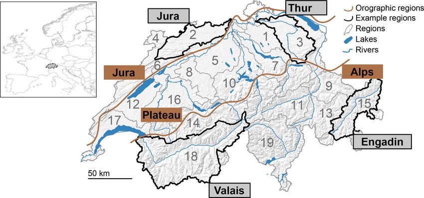
Figure 1. Map of Switzerland with 19 large hydrological regions (grey outline) and the four illustration regions (black border): Thur, Jura,
Valais, and Engadin. The main orographic regions Jura, Plateau, and Alps are outlined by the brown lines.
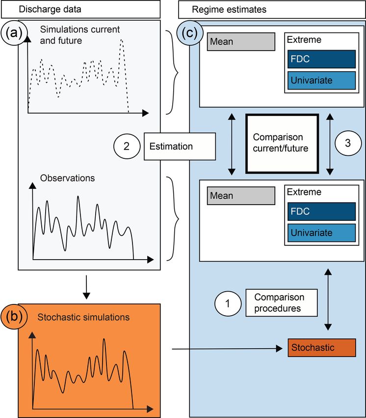
time series using the approach proposed by Brunner et al. 2.2 Analysis framework
(2019a) (provided in the R-package PRSim, which can be
found in the CRAN repository https://cran.r-project.org/web/
packages/PRSim/index.htmlapproaches, last access: 7 Oc- The analysis performed to detect changes in future extreme
tober 2019). As opposed to classical phase randomization, regimes consisted of three main steps (Fig. 2). First, dif-
this approach does not rely on the empirical distribution, but ferent procedures for estimating extreme flow regimes were
uses the flexible, four-parameter kappa distribution (Hosk- tested (first step). Once a suitable procedure was identified, it
ing, 1994), which allows for the generation of a wide range of was applied to estimate extreme high- and low-flow regimes
realizations of high and low discharge values. Among these under current and future climate conditions (second step).
simulated series, extreme regimes can be identified. After These extreme regimes were compared to mean regimes.
having identified a suitable approach for the estimation of Third, current and future estimates were compared to detect
extreme regimes, we apply this approach to discharge time future changes in flow regimes (third step). We used simu-
series representing future climate conditions. A comparison lated discharge representing both current and future climatol-
to current estimates allows us to identify future changes in ogy as the basis for the analysis. The current discharge series
extreme high- and low-flow regimes. were derived by feeding a hydrological model with observed
meteorological data and with meteorological data simulated
by a set of climate models for the reference period. The fu-
2 Methods ture discharge series were obtained by driving the model with
meteorological data from downscaled and bias-corrected cli-
2.1 Study area
mate model simulations.
The analyses were performed on a set of 19 hydrological re- The two estimation techniques applied use frequency anal-
gions in Switzerland (Fig. 1) with areas between 600 and ysis of different quantities. The first method applies fre-
5000 km2 , mean elevations between 550 and 2300 m a.s.l., quency analysis to the individual percentiles of the FDC.
and mean annual precipitation sums between 1000 and The second method uses stochastically simulated discharge
1800 mm. The flow regimes north of the Alps (Plateau and time series to identify annual hydrographs with a certain non-
Jura) are dominated by rainfall and characterized by high dis- exceedance probability. We refer to these methods as FDC
charge in winter and spring but low discharge in summer. In and stochastic, respectively. The two methods are compared
contrast, the regimes in the Alps are dominated by snowmelt to a benchmark method (univariate), which performs uni-
and ice melt and characterized by high discharge in sum- variate frequency analysis of the monthly discharge values
mer. For illustration purposes, we chose four regions. Two of and neglects the dependence between individual months. We
them (Jura and Thur) have a rainfall-dominated regime and here focus on the estimation of high- and low-flow regimes
the other two (Valais and Engadin) a melt-dominated regime with a return period of T = 100 years since this return pe-
under the current climate. riod is commonly used for planning purposes. The methods
outlined in this study, however, can be generalized to other
return periods. In the following paragraphs, we describe the
data sets (Fig. 2a, Sect. 2.3), the stochastic discharge gen-
eration procedure (Fig. 2b, Sect. 2.4), and the estimation
www.hydrol-earth-syst-sci.net/23/4471/2019/ Hydrol. Earth Syst. Sci., 23, 4471–4489, 2019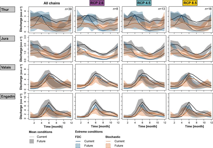
4474                                                             M. I. Brunner et al.: Extreme, current, and future runoff regimes

                                                                         tion was conducted over the period 1993–1997. Validation on
                                                                         discharge was performed with the period 1983–2005. More
                                                                         details on the calibration and validation procedures can be
                                                                         found in Köplin et al. (2010). The parameters for each model
                                                                         grid cell were derived by regionalizing the parameters ob-
                                                                         tained for the 140 catchments with ordinary kriging (Viviroli
                                                                         et al., 2009a; Köplin et al., 2010). The hydrological model
                                                                         has been calibrated using observed meteorological data, but
                                                                         will subsequently be fed with meteorological data simulated
                                                                         by a set of GCM–RCM combinations. It is assumed that the
                                                                         parameter set derived in the calibration procedure will still
                                                                         produce reliable results since Krysanova et al. (2018) have
                                                                         confirmed in a review that a good performance of hydro-
                                                                         logical models in the historical period increases confidence
                                                                         in projected impacts under climate change. Future glacier
                                                                         extents were simulated with two glacier evolution models.
                                                                         We used the global glacier evolution model (GloGEM; Huss
                                                                         and Hock, 2015) for short glaciers (glacier length < 1 km)
                                                                         and GloGEMflow (Zekollari et al., 2019) for long glaciers
                                                                         (length > 1 km). GloGEM simulates glacier changes with a
                                                                         retreat parameterization relying on observed glacier changes
                                                                         (Huss et al., 2010). GloGEMflow is an extended version
                                                                         of GloGEM with a dynamic ice flow component. This new
Figure 2. Illustration of the study framework. (1) Comparison of
                                                                         model was extensively validated over the European Alps
the different estimation techniques univariate, FDC, and stochas-        through comparisons with various observations (e.g., sur-
tic, (2) estimation of current and future mean and extreme regimes       face velocities and observed glacier changes) and detailed 3-
using simulated discharge time series, and (3) comparison of cur-        D projections from modeling studies focusing on individual
rent and future regime estimates. The paper (a) introduces the sim-      glaciers (e.g., Jouvet et al., 2011; Zekollari et al., 2014). The
ulated data used, (b) outlines the stochastic discharge generator, and   simulated glacier extents were transformed from the Glo-
(c) describes the estimation approaches.                                 GEM(flow) 1-D model grid to the 2-D PREVAH model grid
                                                                         by ensuring that the area for each elevation band was con-
                                                                         served.
techniques used to derive extreme flow regimes (Fig. 2c,                    PREVAH is driven by time series of precipitation, temper-
Sect. 2.5).                                                              ature, relative humidity, shortwave radiation, and wind speed.
                                                                         The meteorological forcing for current simulations was ob-
2.3    Hydrological simulations                                          served time series provided by the Federal Office of Meteo-
                                                                         rology and Climatology MeteoSwiss (2018), while the tran-
We used discharge time series simulated with the PRE-                    sient meteorological forcing for future simulations was de-
VAH hydrological model (Viviroli et al., 2009b) as input                 rived from the CH2018 climate scenarios (National Centre
for the analysis. To represent current conditions, the model             for Climate Services, 2018). The meteorological data were
was driven with observed meteorological data for the pe-                 interpolated to a 2 × 2 km grid using detrended inverse dis-
riod 1981–2010. To represent future conditions, it was driven            tance weighting where the detrending was based on a re-
with meteorological data obtained by regional climate model              gression between climate variables and elevation (Viviroli
simulations for the period 2071–2100 (see below). PREVAH                 et al., 2009b). The climate scenarios are based on the re-
is a conceptual process-based model. It consists of several              sults from the EURO-CORDEX initiative (Jacob et al., 2014;
sub-models representing different parts of the hydrological              Kotlarski et al., 2014), which are the most sophisticated
cycle: interception storage, soil water storage and depletion            and high-resolution coordinated climate simulations over Eu-
by evapotranspiration, groundwater, snow accumulation and                rope. The scenarios are based on representative concentra-
snowmelt and glacier melt, runoff and baseflow generation,               tion pathways (RCPs) (Moss et al., 2010; Meinshausen et al.,
plus discharge concentration and flow routing (Viviroli et al.,          2011; van Vuuren et al., 2011) and a regional downscaling
2009b). A gridded version of the model at a spatial resolution           approach based on quantile mapping (Themeßl et al., 2012;
of 200 m was set up for Switzerland (Speich et al., 2015). For           Gudmundsson et al., 2012). The quantile mapping procedure
the calibration of the model parameters, meteorological and              was calibrated on the period 1981–2010 and performed on a
discharge time series from 140 mesoscale catchments cov-                 grid-by-grid basis for all meteorological variables. The mete-
ering different runoff regimes were used. The model calibra-             orological data were derived from an ensemble of 39 GCM–

Hydrol. Earth Syst. Sci., 23, 4471–4489, 2019                                          www.hydrol-earth-syst-sci.net/23/4471/2019/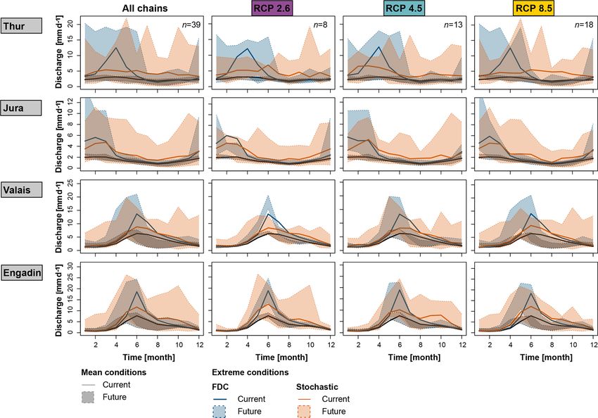
M. I. Brunner et al.: Extreme, current, and future runoff regimes                                                                   4475

RCM combinations for different scenarios (Table A1 in the                   served. In a third step, the inverse Fourier transform is ap-
Appendix), which provide temperature, precipitation, rela-                  plied to transform the data from the spectral domain back
tive humidity, shortwave radiation, and wind speed for the                  to the temporal domain. A step-by-step description of the
locations of various meteorological stations. The selection                 stochastic simulation procedure and more background in-
of scenarios included the three RCPs2.6, 4.5, and 8.5 for                   formation on the Fourier transform are provided in Brunner
which 8, 13, and 18 GCM–RCM combinations were avail-                        et al. (2019a), and references therein. An application of the
able, respectively. Ten out of the 39 GCM–RCM combina-                      simulation procedure to four example catchments in Switzer-
tions were available at a high resolution of 12.5 km and the                land has shown that both seasonal statistics and temporal
remaining combinations at a resolution of roughly 50 km.                    correlation structures of discharge can be well reproduced
Using combinations at both resolutions allows for a larger                  (Brunner et al., 2019a). We therefore used this method to
ensemble; however, it means that those GCM–RCM combi-                       stochastically simulate 1500 years of discharge for each of
nations which are available for both resolutions obtain more                the 19 regions in our data set. Stochastic series representing
weight. During a model run, PREVAH reads the meteoro-                       current conditions were generated by using the hydrological
logical grids and further downscales the data to the compu-                 model simulations for 1981–2010 obtained by the 39 GCM–
tational grid of 200 × 200 m using bilinear interpolation. For              RCM combinations as input. Stochastic series representing
temperature, a lapse rate of −0.65 ◦ C/100 m was additionally               future conditions were generated based on each of the hydro-
used for topographic corrections.                                           logical model simulations generated with the 39 GCM–RCM
                                                                            combinations for different scenarios.
2.4   Stochastic simulation of discharge time series
                                                                            2.5     Estimation of T -year hydrographs
The discharge simulated with the hydrological model for the
current (1981–2010) and future (2071–2100) 30-year peri-                    We employed two methods for estimating 100-year low- and
ods only represents small sets of possible annual hydrograph                high-flow regimes: FDC and stochastic. The extreme regime
realizations. Among these realizations, certain hydrographs                 estimates were compared to the stochastically generated hy-
including extreme hydrographs such as a 100-year hydro-                     drographs to check for plausibility. Furthermore, they were
graph were possibly not observed. We used a stochastic dis-                 compared to a lower-bound (for low-flow regimes) or upper-
charge simulation procedure to increase the number of pos-                  bound (for high-flow regimes) benchmark regime derived by
sible annual hydrograph realizations. These realizations rep-               combining 100-year monthly discharge estimates obtained
resent the discharge statistics and temporal correlation struc-             from univariate frequency analysis. This frequency analy-
ture of the available data and extend the existing sample to as             sis was performed on the values of each month indepen-
yet unobserved annual hydrographs. To simulate such hydro-                  dently and the monthly values were fitted with a general-
graphs, we used the method of phase randomization (Theiler                  ized extreme value (GEV) distribution. This distribution was
et al., 1992; Schreiber and Schmitz, 2000). We combined this                not rejected according to the Anderson–Darling goodness-
empirical procedure with the flexible four-parameter kappa                  of-fit test computed using the procedure proposed by Chen
distribution (Hosking, 1994) to allow for the extrapolation                 and Balakrishnan (1995) (α = 0.05). The disadvantage of the
to as yet unobserved values. This phase randomization ap-                   univariate procedure is that the autocorrelation in the data,
proach preserves the autocorrelation structure of the raw se-               which is mainly visible for lags of 1 and 2 months, is ne-
ries by conserving its power spectrum (Theiler et al., 1992).               glected, which overestimates the extremeness of the 100-
The procedure consists of three main steps (Radziejewski                    year low-flow regime and therefore produces unrealistic es-
et al., 2000). In a first step, the discharge series (here, the             timates. The univariate approach will therefore only be con-
simulated discharge for past and future conditions) is con-                 sidered as a benchmark for model comparison and will not
verted from the time domain to the spectral domain by the                   find consideration in the comparison of current and future
Fourier transform (Morrison, 1994). The Fourier transform                   extreme regime estimates.
of a given time series x = (x1 , . . . , xt , . . . , xn ) of length n is
                  n                                                         2.5.1    FDC
             1    X
                             −iωt
f (ω) = √                e          xt , −π ≤ ω ≤ π,                 (1)
         2π n      t=1                                                      A first extreme regime estimate was derived by performing
                                                        √                   the frequency analysis of annual FDCs. According to Vo-
where t is the time step, ω are the phases, and i = −1 is                   gel and Fennessey (1994), an annual FDC with an assigned
the imaginary unit. In this spectral domain, the data are repre-            return period can be obtained from the pth quantile func-
sented by the phase angle and by the amplitudes of the power                tion. To do so, we fitted a GEV distribution to the quan-
spectrum as represented by the periodogram. The phase an-                   tiles corresponding to each percentile. The GEV was not re-
gle of the power spectrum is uniformly distributed over the                 jected based on the Anderson–Darling goodness-of-fit test
range −π to π . In a second step, the phases in the phase                   (α = 0.05). The fitted GEV distributions were used to esti-
spectrum are randomized, while the power spectrum is pre-                   mate the 100-year quantile for each percentile. The 100-year

www.hydrol-earth-syst-sci.net/23/4471/2019/                                                Hydrol. Earth Syst. Sci., 23, 4471–4489, 2019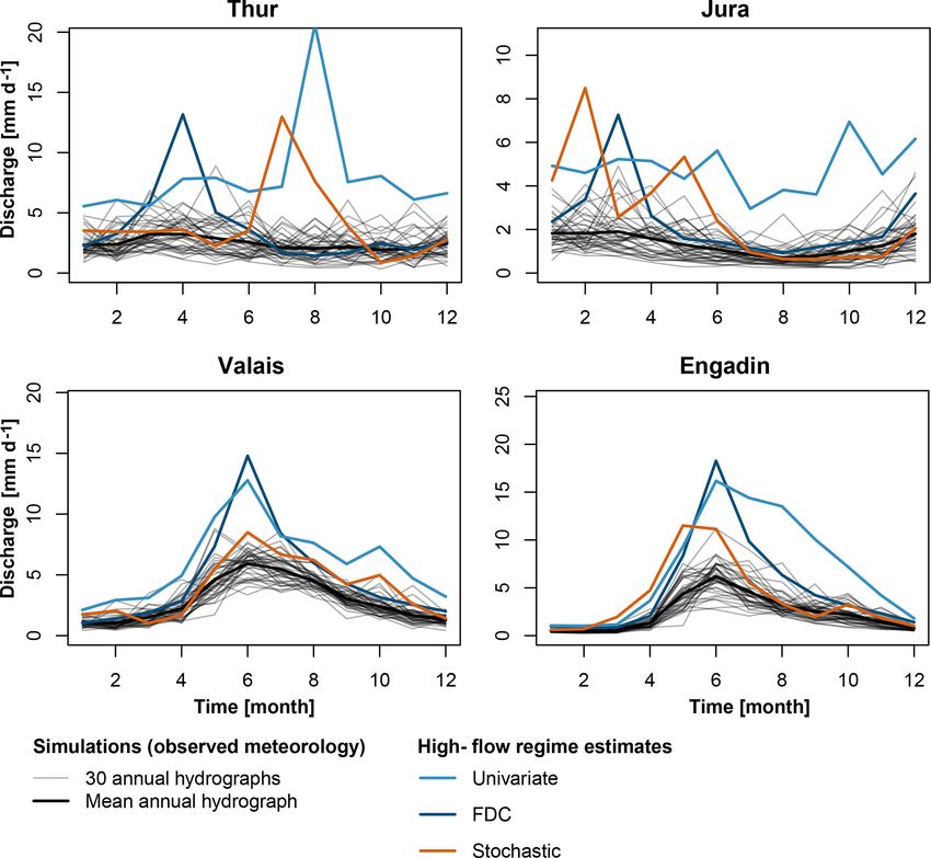
4476                                                      M. I. Brunner et al.: Extreme, current, and future runoff regimes

FDC was then derived by combining these 100-year quan-
tiles. The 100-year FDC does not contain any information
about the seasonality, but only about the statistical distribu-
tion of flow. To include information about seasonality, we
combined the estimated 100-year FDC with a typical sea-
sonal regime. To do so, the individual quantile values of the
FDC were assigned to the corresponding ranks of a typical
flow regime. This typical regime was defined as the long-
term (mean) regime of the daily input time series and varied
for current and future conditions. The estimated extreme dis-
charge regimes were aggregated to a monthly resolution to         Figure 3. Illustration of the main characteristics of an annual
make them comparable to the univariate estimates.                 rainfall-dominated flow regime under current and future conditions:
                                                                  maximum, mean, and minimum.
2.5.2    Stochastic

The second method for the estimation of extreme regimes           3     Results
performs the frequency analysis directly on a large
set of stochastically simulated annual hydrographs (here          3.1    Comparison of estimation methods
1500 years). The frequency analysis was performed on the
annual sums of the stochastically generated hydrographs.          The two estimation techniques and the benchmark approach
We identified the hydrograph corresponding to the empiri-         provide distinct estimates for the 100-year low-flow regimes
cal 100-year annual discharge sum as the 100-year regime.         (Fig. 4). The univariate technique leads to the most extreme
The application of this procedure is only possible for long       regimes, whilst the FDC and stochastic methods lead to sim-
time series as given by the stochastic series, since a 100-year   ilar estimates. The univariate estimate should only be seen as
annual sum is not necessarily observed in a short record of,      a lower benchmark and not as an estimate for a “true” 100-
say, 30 years. Like the FDC estimates, the regimes derived        year regime since the univariate approach neglects the de-
from the stochastic approach were aggregated to a monthly         pendence between monthly estimates. In contrast, the FDC
resolution.                                                       and stochastic approaches produce more plausible estimates,
                                                                  i.e., estimates at the lower bound of the observed values. The
2.6     Comparison of current and future regime estimates
                                                                  summer low-flow regimes estimated by the FDC technique
The two methods and the benchmark approach for the es-            are comparable to the regimes of the year 2003, which in-
timation of 100-year low- and high-flow regime estimates          cluded a very dry summer (Beniston, 2004; Rebetez et al.,
were applied to discharge time series representing current        2006; Schär et al., 2004; Zappa and Kan, 2007).
and future climate conditions. First, 100-year regimes were          Similarly to low-flow regimes, the 100-year high-flow
estimated for current conditions (1981–2010). To generate         regimes derived by the three estimation techniques are dis-
a control regime, we used the discharge simulated with the        tinct (Fig. 5). The univariate approach, as mentioned pre-
observed meteorological data. To represent uncertainty due        viously, produces unrealistic results in terms of seasonal-
to different GCM–RCM combinations for different scenar-           ity, since the predictions of the monthly 100-year flows ne-
ios, we derived one reference regime for each discharge time      glect the dependence between the different months. The FDC
series simulated by the 39 climate GCM–RCM combinations           and stochastic techniques produce more similar seasonalities
for different scenarios. This analysis provided us with a range   and more realistic estimates at the upper bound of the ob-
of current regime estimates due to climate model uncertainty.     served annual hydrographs. Contrary to low-flow estimates,
The regime estimates derived from the 39 GCM–RCM com-             high-flow estimates generated with the FDC or stochastic
binations were used to derive a multi-model mean, which           techniques can be different. The stochastic approach gener-
served as a reference for determining changes between cur-        ally leads to more conservative estimates than the FDC ap-
rent and future conditions. In a second step, 100-year esti-      proach in melt-dominated regions. We attribute this to the
mates were derived for future conditions using the simulated      fact that the stochastic approach performs frequency analysis
time series for the period 2071–2100 for all GCM–RCM              of annual sums, while the FDC approach performs frequency
combinations and scenarios. We assessed changes in season-        analysis of the percentiles of the FDC.
ality and magnitude of flow regimes in terms of their mini-          The plausibility of the 100-year estimates derived by using
mum, maximum, and mean discharges by comparing regime             the FDC and stochastic approaches is shown by a comparison
estimates derived for future conditions to the multi-model        with stochastically generated annual hydrographs (Fig. A1 in
mean representing current conditions. (Figure 3; results were     the Appendix for the low-flow estimates). The derived esti-
grouped by RCP.)                                                  mates, in fact, are embedded in the lower spectrum of the
                                                                  stochastically generated annual hydrographs. This is hardly

Hydrol. Earth Syst. Sci., 23, 4471–4489, 2019                                     www.hydrol-earth-syst-sci.net/23/4471/2019/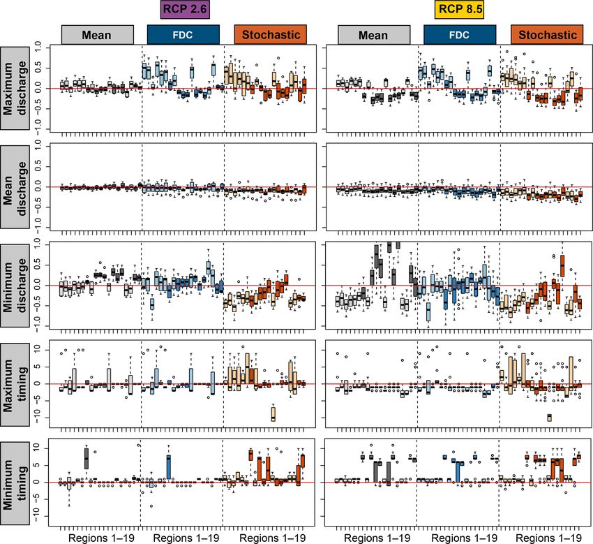
M. I. Brunner et al.: Extreme, current, and future runoff regimes                                                                    4477

Figure 4. 100-year low-flow regime estimates for current climate conditions (control) derived using univariate frequency analysis (light
blue), frequency analysis of the FDC (dark blue), and stochastically generated time series (orange). The annual hydrographs simulated using
observed meteorological data are given in grey, while the mean annual hydrograph and the hydrograph simulated for the year 2003 are given
in black. The four panels are shown on different scales.

the case for the univariate estimates, which lead to “unre-             model output realistically reproduces the observed climate.
alistically low” 100-year hydrographs partly outside of the             An exception is the Engadin, where the low-flow regimes de-
range of the stochastically generated hydrographs. Similarly,           rived from the GCM–RCM combinations overestimate sum-
the 100-year high-flow regime estimates derived by the FDC              mer low flows. This overestimation might be related to the
and stochastic methods are embedded in the higher spectrum              univariate bias correction applied, which might not perfectly
of the stochastically generated hydrographs, while the uni-             reflect the interplay between temperature and precipitation
variate estimate is “unrealistically high”. Since the univariate        and therefore the timing of snowmelt processes (Meyer et al.,
approach yields unrealistic estimates, it is not considered for         2019). The spread in the current regimes is larger for extreme
further analysis.                                                       than for mean conditions for the rainfall-dominated catch-
                                                                        ments Thur and Jura. In addition, the spread is larger for the
3.2   Current and future low-flow regime estimates                      high- than for the low-flow extreme regimes except for the
                                                                        Engadin region. This range should be kept in mind when an-
Both mean and extreme regimes are subject to uncertainty                alyzing future regime estimates.
when derived from simulated discharge. The uncertainty                     Shifts in regimes are expected for both mean and extreme
comes from the hydrological model and from the spread be-               low-flow conditions (Fig. 7). The shifts are weak for rainfall-
tween the climate simulations. Figure 6 shows mean and ex-              dominated regions (e.g., Thur and Jura), while they are strong
treme low- and high-flow regime estimates derived for the               for melt-dominated regions (e.g., Valais and Engadin). For
observed climatology for the four illustration catchments. It           the rainfall-dominated regions, changes in mean and extreme
also shows the range of regimes obtained by using differ-               regimes are most visible for RCP8.5. Here, the different real-
ent GCM–RCM combinations and scenarios. This range of                   izations lead to regimes with more pronounced summer low
regimes generally encompasses the regime derived from me-               flows. In addition, there is a reduction in spring discharge
teorological observations, which suggests that the climate              under RCP2.6 for both mean and extreme conditions when

www.hydrol-earth-syst-sci.net/23/4471/2019/                                           Hydrol. Earth Syst. Sci., 23, 4471–4489, 2019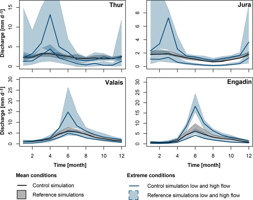
4478                                                         M. I. Brunner et al.: Extreme, current, and future runoff regimes

Figure 5. 100-year high-flow regime estimates for current conditions (control) derived using univariate frequency analysis (light blue),
frequency analysis of the FDC (dark blue), and stochastically generated time series (orange). The annual hydrographs simulated using
observed meteorological data are given in grey, while the mean annual hydrograph is given in black. The four panels are shown on different
scales.

looking at the regimes derived from the FDC approach. In               In contrast, a decrease is expected in the discharge minimum
the case of melt-dominated regions, most GCM–RCM com-                  according to the stochastic approach, while no clear changes
binations lead to clear shifts towards regimes with earlier and        are expected using the FDC approach. For melt-dominated
reduced summer flows. These shifts are more pronounced for             regions, the change pattern is different. There, a decrease in
RCP8.5 than RCPs4.5 and 2.6. Note that the spread of future            maximum discharge is expected. An increase in minimum
regimes is smaller for RCP2.6 than RCPs4.5 and 8.5 due to              discharge is expected for mean regimes, while changes are
the smaller number of chains in the ensemble.                          less clear for the extreme regimes. Shifts of 1 or 2 months
   Differences between current (i.e., multi-model mean of              are expected in timing for both rainfall- and melt-dominated
reference simulations) and future mean and extreme low-                regions. In most catchments, the timing of future maximum
flow regimes are summarized in Fig. 8. The detected changes            discharge is likely to occur earlier than under current con-
for RCP2.6 and RCP8.5 are similar (results for RCP4.5 are              ditions. Shifts towards later in the year are expected in the
not displayed, but lie in between those of RCPs2.6 and 8.5).           timing of the minimum flow. The changes in mean and max-
Changes are projected for the minimum and maximum dis-                 imum flows are similar for extreme low-flow regimes derived
charges of mean and extreme low-flow regimes and for their             by the two estimation techniques FDC and stochastic. In con-
timing, but less for the mean of these regimes. The changes            trast, the shifts in minimum flow and timing are different
in the mean flow can reach up to 30 %, while the maximum               when applying the stochastic approach instead of the FDC
and minimum flows can change up to 100 %.                              approach.
   Changes in melt- and rainfall-dominated regions are
clearly different. Both the FDC and stochastic approach                3.3   Current and future high-flow regime estimates
suggest changes in extreme low-flow regimes. In rainfall-
dominated regions, an increase is expected for the discharge           High-flow regime estimates are also expected to change
maximum independent of the estimation approach chosen.                 (Fig. 9), with no consistent change pattern visible at first

Hydrol. Earth Syst. Sci., 23, 4471–4489, 2019                                         www.hydrol-earth-syst-sci.net/23/4471/2019/
M. I. Brunner et al.: Extreme, current, and future runoff regimes                                                                  4479

Figure 6. Current 100-year mean regimes (grey), low-flow regimes (blue lower line), and high-flow regimes (blue upper line) estimated by
using the FDC method on the control discharge simulations derived by observed meteorological data (bold line) and the reference discharge
simulations derived by meteorological data simulated by the 39 GCM–RCM combinations for different scenarios for the reference period
(shaded polygons).

Figure 7. Comparison of current multi-model mean (solid line) and future 100-year low-flow regime estimates (shaded polygons) over the
39 GCM–RCM combinations and scenarios derived by the FDC (blue) and stochastic (orange) approaches. The mean regimes are provided
as a reference (grey).

www.hydrol-earth-syst-sci.net/23/4471/2019/                                          Hydrol. Earth Syst. Sci., 23, 4471–4489, 2019
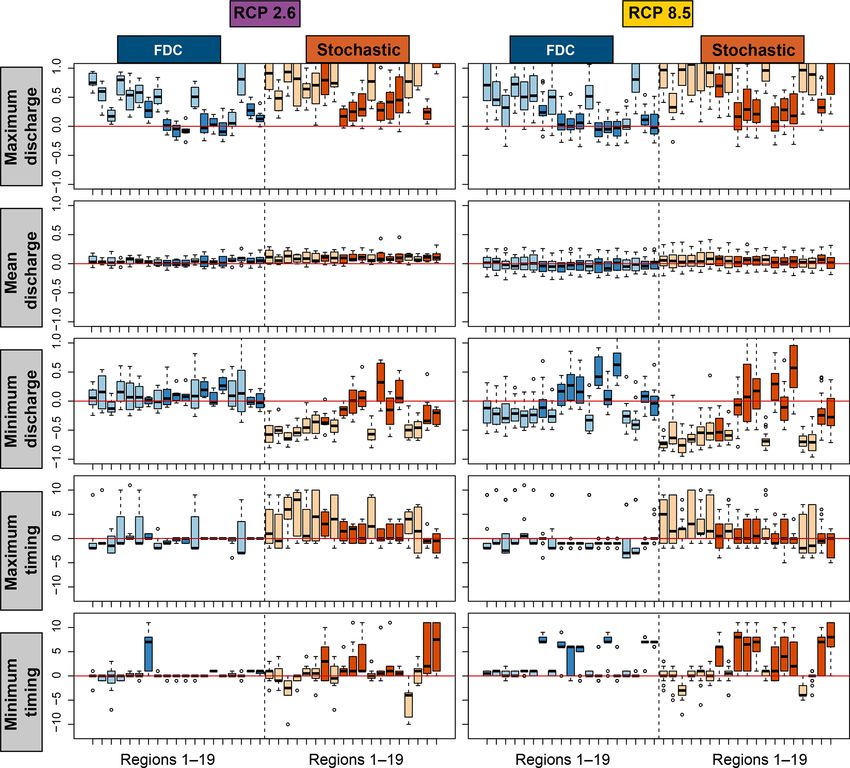
4480                                                           M. I. Brunner et al.: Extreme, current, and future runoff regimes

Figure 8. Differences between current (i.e., multi-model mean of reference simulations) and future mean (grey) and extreme low-flow
regime characteristics for the 19 regions (Fig. 1) estimated by the FDC (blue) and stochastic (orange) approaches. Five indicators are shown:
maximum discharge, mean discharge, minimum discharge, timing of minimum discharge, and timing of maximum discharge. The first three
rows show relative changes, the last two rows changes in months. Melt-dominated (dark colors) and rainfall-dominated regions (light colors)
are distinguished. The boxplots indicate the range resulting from using the 39 GCM–RCM combinations for different scenarios.

glance. Changes in high-flow extreme regimes are slightly                are much stronger, i.e., up to 100 %. In rainfall-dominated
more pronounced for RCP8.5 than for RCP2.6 (Fig. 10;                     regions, changes in maximum discharge are mostly posi-
RCP4.5 not shown because it is expected to provide results               tive, while they can be negative for melt-dominated regions.
somewhere in between RCPs2.6 and 8.5). They are simi-                    In these melt-dominated regions, an increase is expected in
lar for the estimation techniques used (FDC/stochastic). As              the minimum discharge of high-flow extreme regimes, espe-
for the low-flow regimes, only moderate and mostly posi-                 cially when using the FDC approach. In rainfall-dominated
tive changes of less than 30 % are expected in the mean dis-             regions, changes in minimum discharge are mostly negative,
charge of extreme high-flow regimes. The changes in the                  especially for RCP8.5. Changes in timing are different for the
maximum and minimum discharges of the high-flow regimes                  FDC and stochastic approach and there is no consistent pat-

Hydrol. Earth Syst. Sci., 23, 4471–4489, 2019                                           www.hydrol-earth-syst-sci.net/23/4471/2019/
M. I. Brunner et al.: Extreme, current, and future runoff regimes                                                                4481

Figure 9. Comparison of current multi-model mean (solid line) and future 100-year high-flow regime estimates (shaded polygons) over the
39 GCM–RCM combinations derived by the FDC (blue) and stochastic (orange) approaches. The mean regimes are provided as a reference
(grey).

tern across catchments. Minimum and maximum discharges                derived from the two estimates are similar except for changes
can occur earlier or later in the year than under current con-        in minimum discharge in the low-flow regime and minimum
ditions.                                                              discharge in the high-flow regimes. Both types of estimates
                                                                      seem to be plausible in the light of the stochastically gener-
                                                                      ated hydrographs, which represent a large set of possible re-
4     Discussion                                                      alizations among which extreme hydrographs can be found.
                                                                      While the estimates derived by the two methods do not dif-
4.1    Estimation methods                                             fer much, both methods have their advantages and disad-
                                                                      vantages. The FDC approach is relatively simple to imple-
The low-flow regime estimates derived with the univariate             ment but decouples seasonality from the distribution of daily
method are implausible because the method neglects the in-            discharge values. In contrast, the stochastic approach jointly
terdependence between flows of adjacent months. In con-               considers magnitude and seasonality but requires the imple-
trast, both other methods, FDC and stochastic, lead to similar        mentation of a stochastic discharge generator. The main ad-
results. The differences between the two methods mainly lie           vantage of such a generator is that the individual hydrograph
in how the seasonality is derived. In the case of the FDC ap-         realizations can be used for specific impact studies, which al-
proach, mean seasonality is used. In the case of the stochas-         lows for direct performance of the frequency analysis of the
tic approach, a rather “random” seasonality is used since the         quantity of interest. There are several possible solutions to
regime is chosen according to the annual discharge sum. The           the multivariate problem of estimating extreme regimes, and
use of one potential realization of seasonality in the stochas-       none of these two methods can therefore be said to be the
tic approach compared to the use of a mean seasonality in             better one.
the FDC approach has the disadvantage that it is less repre-             The estimation of extremes, be it of regimes or individ-
sentative but the advantage that it is consistent with the cor-       ual flow characteristics, is associated with several sources of
responding annual discharge sum. The direction of changes

www.hydrol-earth-syst-sci.net/23/4471/2019/                                        Hydrol. Earth Syst. Sci., 23, 4471–4489, 2019
4482 M. I. Brunner et al.: Extreme, current, and future runoff regimes Figure 10. Differences between current (i.e., multi-model mean of reference simulations) and future mean (grey) and extreme high-flow regime characteristics for the 19 regions (Fig. 1) estimated by the FDC (blue) and stochastic (orange) approaches. Five indicators are shown: maximum discharge, mean discharge, minimum discharge, timing of minimum discharge, and timing of maximum discharge. The first three rows show relative changes, the last two rows changes in months. Melt-dominated (dark colors) and rainfall-dominated (light colors) regions are distinguished. The boxplots indicate the range resulting from using the 39 GCM–RCM combinations for different scenarios. uncertainty. These comprise the choice of an extreme value ent in the hydrological model results, and the calibration of distribution used to fit the data (i.e., percentiles of FDCs, an- its parameters (Wilby et al., 2008; Addor et al., 2014; Clark nual sums, daily discharge sums) and the estimation of its et al., 2016). Despite these uncertainties, the extreme regime parameters (Merz and Thieken, 2005; Brunner et al., 2018a). estimates can be used to identify future changes, and as such When applied to time series representing future conditions these estimates can be further used in climate impact stud- simulated with a hydrological model, additional uncertainty ies. Potential fields of application include water scarcity as- sources are involved. These include the assumptions under- sessments, where such regime estimates are combined with lying the applied future global climate scenarios, global cli- estimates of water demand (Brunner et al., 2018b), eco- mate model structures, initial conditions, downscaling meth- hydrological studies (Wood et al., 2008), or analyses of the ods, modeled future glacier extents, the uncertainties inher- Hydrol. Earth Syst. Sci., 23, 4471–4489, 2019 www.hydrol-earth-syst-sci.net/23/4471/2019/
M. I. Brunner et al.: Extreme, current, and future runoff regimes 4483
future potential of hydropower production (Schaefli et al., 5 Conclusions
2019).
Extreme regime estimates were derived by frequency anal-
4.2 Changes in future regime estimates ysis performed on (1) annual flow duration curves (FDCs)
and (2) the discharge sums of stochastically generated an-
Changes in all types of regimes (mean/extreme low nual hydrographs. Both were found to provide realistic, sim-
flow/extreme high flow) were found to be distinct for melt- ilar results. A range of future extreme regime estimates was
dominated and rainfall-dominated regions. This refers not obtained for both extreme and mean conditions. In rainfall-
only to the entire regime, but also to individual regime char- dominated regions, the range of these future low- and high-
acteristics such as minimum, maximum, and mean flow as flow estimates comprised the current estimate. In contrast,
well as the timing of the minimum flow. The direction of in melt-dominated regions, future high-flow and especially
change was different in rainfall- and melt-dominated regions low-flow regimes were distinct from the current estimate.
for all regime types. An increase of up to 50 % in the maxi- Changes in mean discharges were moderate for all types
mum discharge of mean and extreme low- and extreme high- of regimes and catchments and did not exceed 30 %. Pro-
flow regimes was found for rainfall-dominated regions. In jected changes in the minimum discharge of mean and ex-
contrast, a decrease in the minimum discharge by up to treme high- and low-flow regimes were positive in melt-
100 % is projected to occur for these catchments and all dominated regions due to increases in winter precipitation
types of regimes. The opposite is true for melt-dominated and amount to up to 100 %. In contrast, mostly positive
regimes, where the minimum discharge increases while the changes of up to 50 % in maximum discharge were found
maximum and mean discharges decrease. The changes in ex- in rainfall-dominated regions for all types of regimes. These
treme regimes can be explained by a reduction or an earlier positive changes in maximum discharge are linked to in-
contribution of snowmelt and glacier melt (Hanzer et al., creases in winter precipitation, which coincide with the high-
2018) and by an increase in winter precipitation (Jenicek flow season. High- and low-flow regime estimates derived
et al., 2018), which coincide with the high-flow season in using the approaches proposed in this study are important
rainfall-dominated regions but with the low-flow season in for climate impact studies addressing, e.g., the future hy-
melt-dominated regions. For mean regimes, changes in melt- dropower production potential or the occurrence of water
dominated regimes were found in previous studies (Barnett shortage situations. The estimates also provide guidance for
et al., 2005; Jenicek et al., 2018; Fatichi et al., 2014; Hanzer hydraulic design, emergency planning, and drought and wa-
et al., 2018). Fatichi et al. (2014) found a projected discharge ter management.
decrease in melt-dominated regions due to reduced contri-
bution of ice melt in the Po and Rhine river basins. The
regime shifts in the rainfall-dominated regions are also in- Data availability. The climate model simulations are available on
fluenced by increases in precipitation in the winter season the web page of the Swiss National Centre for Climate Services
and decreases in the summer season. Precipitation increases (https://www.nccs.admin.ch/nccs/de/home.html, NCCS, 2018). The
in the high-flow winter season lead to increases in the dis- hydrological model simulations are available upon request from
charge maximum, while precipitation decreases in the low- Massimiliano Zappa (massimiliano.zappa@wsl.ch). The extreme
flow summer season lead to decreases in the discharge mini- regime estimates are available upon request from Manuela I. Brun-
ner (manuela.brunner@wsl.ch).
mum. The results of Fatichi et al. (2014) confirm that changes
in rainfall-dominated regions are more uncertain since the
projected changes in precipitation mostly lie within the range
of natural variability of the control scenario. Similar results
were found by Jenicek et al. (2018) for several catchments
in Switzerland and by Barnett et al. (2005) on a global scale.
We have shown here that these previous findings also apply
to extreme regimes. The regime shifts detected have impli-
cations for various sectors. Regime shifts and more severe
low flows were found to lead to more severe water scarcity
situations, where water supply is insufficient to meet water
demand (Brunner et al., 2019b). In the hydropower sector,
future regime shifts are anticipated to lead to a reduction in
production (Finger et al., 2012; Schaefli et al., 2019).
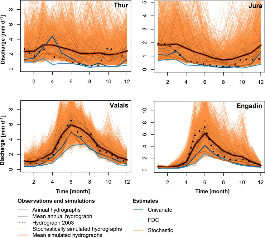
www.hydrol-earth-syst-sci.net/23/4471/2019/ Hydrol. Earth Syst. Sci., 23, 4471–4489, 20194484 M. I. Brunner et al.: Extreme, current, and future runoff regimes Appendix A Figure A1. Comparison of the 100-year low-flow regime estimates univariate, FDC, and stochastic with stochastically generated hydrographs (orange lines). The observed mean hydrograph (solid line) and the hydrograph of the year 2003 (dotted line) are given in black. Hydrol. Earth Syst. Sci., 23, 4471–4489, 2019 www.hydrol-earth-syst-sci.net/23/4471/2019/
M. I. Brunner et al.: Extreme, current, and future runoff regimes                                                            4485

Table A1. Summary of the 39 climate chains considered: global circulation model (GCM), regional climate model (RCM), representative
concentration pathway (RCP), and grid cell resolution.

                               GCM                      RCM                      RCP    Resolution
                               ICHEC-EC-EARTH           DMI-HIRHAM5               2.6     EUR-11
                               ICHEC-EC-EARTH           DMI-HIRHAM5               4.5     EUR-11
                               ICHEC-EC-EARTH           DMI-HIRHAM5               8.5     EUR-11
                               ICHEC-EC-EARTH           SMHI-RCA4                 2.6     EUR-11
                               ICHEC-EC-EARTH           SMHI-RCA4                 4.5     EUR-11
                               ICHEC-EC-EARTH           SMHI-RCA4                 8.5     EUR-11
                               MOHC-HadGEM2-ES          SMHI-RCA4                 4.5     EUR-11
                               MOHC-HadGEM2-ES          SMHI-RCA4                 8.5     EUR-11
                               MPI-M-MPI-ESM-LR         SMHI-RCA4                 4.5     EUR-11
                               MPI-M-MPI-ESM-LR         SMHI-RCA4                 8.5     EUR-11
                               ICHEC-EC-EARTH           CLMcom-CCLM5-0-6          8.5     EUR-44
                               MOHC-HadGEM2-ES          CLMcom-CCLM5-0-6          8.5     EUR-44
                               MIROC-MIROC5             CLMcom-CCLM5-0-6          8.5     EUR-44
                               MPI-M-MPI-ESM-LR         CLMcom-CCLM5-0-6          8.5     EUR-44
                               ICHEC-EC-EARTH           DMI-HIRHAM5               2.6     EUR-44
                               ICHEC-EC-EARTH           DMI-HIRHAM5               4.5     EUR-44
                               ICHEC-EC-EARTH           DMI-HIRHAM5               8.5     EUR-44
                               ICHEC-EC-EARTH           DNMI-RACMO22E             4.5     EUR-44
                               ICHEC-EC-EARTH           DNMI-RACMO22E             8.5     EUR-44
                               MOHC-HadGEM2-ES          DNMI-RACMO22E             2.6     EUR-44
                               MOHC-HadGEM2-ES          DNMI-RACMO22E             4.5     EUR-44
                               MOHC-HadGEM2-ES          DNMI-RACMO22E             8.5     EUR-44
                               CCma-CanESM2             SMHI-RCA4                 4.5     EUR-44
                               CCma-CanESM2             SMHI-RCA4                 8.5     EUR-44
                               ICHEC-EC-EARTH           SMHI-RCA4                 2.6     EUR-44
                               ICHEC-EC-EARTH           SMHI-RCA4                 4.5     EUR-44
                               ICHEC-EC-EARTH           SMHI-RCA4                 8.5     EUR-44
                               MOHC-HadGEM2-ES          SMHI-RCA4                 2.6     EUR-44
                               MOHC-HadGEM2-ES          SMHI-RCA4                 4.5     EUR-44
                               MOHC-HadGEM2-ES          SMHI-RCA4                 8.5     EUR-44
                               MIROC-MIROC5             SMHI-RCA4                 2.6     EUR-44
                               MIROC-MIROC5             SMHI-RCA4                 4.5     EUR-44
                               MIROC-MIROC5             SMHI-RCA4                 8.5     EUR-44
                               MPI-M-MPI-ESM-LR         SMHI-RCA4                 2.6     EUR-44
                               MPI-M-MPI-ESM-LR         SMHI-RCA4                 4.5     EUR-44
                               MPI-M-MPI-ESM-LR         SMHI-RCA4                 8.5     EUR-44
                               NCC-NorESM1-M            SMHI-RCA4                 2.6     EUR-44
                               NCC-NorESM1-M            SMHI-RCA4                 4.5     EUR-44
                               NCC-NorESM1-M            SMHI-RCA4                 8.5     EUR-44

www.hydrol-earth-syst-sci.net/23/4471/2019/                                      Hydrol. Earth Syst. Sci., 23, 4471–4489, 2019
4486 M. I. Brunner et al.: Extreme, current, and future runoff regimes
Author contributions. The idea and setup for the analyses were de- Beniston, M., Farinotti, D., Stoffel, M., Andreassen, L. M., Cop-
veloped by MIB. MZ did the hydrological model simulations. HZ, pola, E., Eckert, N., Fantini, A., Giacona, F., Hauck, C., Huss,
MH, and DF provided the future glacier extents. The analyses were M., Huwald, H., Lehning, M., López-Moreno, J. I., Magnusson,
performed by MIB and discussed with MZ and DF. MIB wrote the J., Marty, C., Morán-Tejéda, E., Morin, S., Naaim, M., Proven-
first draft of the manuscript, which was revised by all the co-authors zale, A., Rabatel, A., Six, D., Stötter, J., Strasser, U., Terzago, S.,
and edited by MIB. and Vincent, C.: The European mountain cryosphere: A review of
its current state, trends, and future challenges, The Cryosphere,
12, 759–794, https://doi.org/10.5194/tc-12-759-2018, 2018.
Competing interests. The authors declare that they have no conflict Berghuijs, W. R., Woods, R. A., Hutton, C. J., and Siva-
of interest. palan, M.: Dominant flood generating mechanisms across
the United States, Geophys. Res. Lett., 43, 4382–4390,
https://doi.org/10.1002/2016GL068070, 2016.
Acknowledgements. We thank MeteoSwiss for providing observed Blöschl, G., Hall, J., Parajka, J., Perdigão, R. A. P., Merz, B.,
meteorological data and the Swiss National Centre for Climate Ser- Arheimer, B., Aronica, G. T., Bilibashi, A., Bonacci, O., Borga,
vices (NCCS) for providing the climate model simulations. M., Ivan, C., Castellarin, A., and Chirico, G. B.: Changing cli-
mate shifts timing of European floods, Science, 357, 588–590,
https://doi.org/10.1126/science.aan2506, 2017.
Brönnimann, S., Rajczak, J., Fischer, E., Raible, C., Rohrer, M.,
Financial support. This research has been supported by the
and Schär, C.: Changing seasonality of moderate and extreme
Swiss Federal Office for the Environment (FOEN) (grant
precipitation events in the Alps, Nat. Hazards Earth Syst. Sci., 18,
no. 15.0003.PJ/Q292-5096).
2047–2056, https://doi.org/10.5194/nhess-18-2047-2018, 2018.
Brunner, M. I., Viviroli, D., Sikorska, A. E., Vannier, O., Favre,
A.-C., and Seibert, J.: Flood type specific construction of syn-
Review statement. This paper was edited by Axel Bronstert and re- thetic design hydrographs, Water Resour. Res., 53, 1390–1406,
viewed by two anonymous referees. https://doi.org/10.1002/2016WR019535, 2017.
Brunner, M. I., Sikorska, A. E., Furrer, R., and Favre, A.-C.: Un-
certainty assessment of synthetic design hydrographs for gauged
and ungauged catchments, Water Resour. Res., 54, WR021129,
https://doi.org/10.1002/2017WR021129, 2018a.
References Brunner, M. I., Zappa, M., and Stähli, M.: Scale matters:
effects of temporal and spatial data resolution on water
Addor, N., Rössler, O., Köplin, N., Huss, M., Weingartner, R., and scarcity assessments, Adv. Water Resour., 123, 134–144,
Seibert, J.: Robust changes and sources of uncertainty in the pro- https://doi.org/10.1016/j.advwatres.2018.11.013, 2018b.
jected hydrological regimes of Swiss catchments, Water Resour. Brunner, M. I., Bárdossy, A., and Furrer, R.: Technical note:
Res., 50, 1–22, https://doi.org/10.1002/2014WR015549, 2014. Stochastic simulation of streamflow time series using phase
Alderlieste, M., Van Lanen, H., and Wanders, N.: Future low flows randomization, Hydrol. Earth Syst. Sci., 23, 3175–3187,
and hydrological drought: How certain are these for Europe?, in: https://doi.org/10.5194/hess-23-3175-2019, 2019a.
Proceedings of FRIEND-Water 2014, vol. 363, IAHS, Montpel- Brunner, M. I., Björnsen Gurung, A., Zappa, M., Zekollari,
lier, 60–65, 2014. H., Farinotti, D., and Stähli, M.: Present and future wa-
Anghileri, D., Voisin, N., Castelletti, A., Pianosi, F., Nijssen, ter scarcity in Switzerland: Potential for alleviation through
B., and Lettenmaier, D.: Value of long-term streamflow fore- reservoirs and lakes, Sci. Total Environ., 666, 1033–1047,
casts to reservoir operations for water supply in snow- https://doi.org/10.1016/j.scitotenv.2019.02.169, 2019b.
dominated river catchments, Water Resour. Res., 52, 4209–4225, Castellarin, A., Vogel, R. M., and Brath, A.: A stochastic index flow
https://doi.org/10.1002/2015WR017864, 2016. model of flow duration curves, Water Resour. Res., 40, 1–10,
Aon Benfield: 2016 annual global climate and catas- https://doi.org/10.1029/2003WR002524, 2004.
trophe report, Tech. rep., Aon Benfield, available at: Chen, G. and Balakrishnan, N.: A general purpose approximate
http://thoughtleadership.aonbenfield.com/Documents/ goodness-of-fit test, J. Qual. Technol., 2, 154–161, 1995.
20170117-ab-if-annual-climate-catastrophe-report.pdf (last Claps, P. and Fiorentino, M.: Probabilistic flow duration curve for
access: 15 March 2019), 2016. use in environmental planning and management, in: Integrated
Arnell, N. W.: The effect of climate change on hydrologi- approach to environmental data management systems, edited by:
cal regimes in Europe, Global Environ. Change, 9, 5–23, Harmancioglu, N. B., Alpaslan, M. N., Ozkul, S. D., and Singh,
https://doi.org/10.1016/S0959-3780(98)00015-6, 1999. V. P., Springer, Dordrecht, 255–266, 1997.
Barnett, T. P., Adam, J. C., and Lettenmaier, D. P.: Po- Clark, M. P., Wilby, R. L., Gutmann, E. D., Vano, J. A., Gangopad-
tential impacts of a warming climate on water avail- hyay, S., Wood, A. W., Fowler, H. J., Prudhomme, C., Arnold,
ability in snow-dominated regions, Nature, 438, 303–309, J. R., and Brekke, L. D.: Characterizing uncertainty of the hy-
https://doi.org/10.1038/nature04141, 2005. drologic impacts of climate change, Curr. Clim. Change Rep., 2,
Beniston, M.: The 2003 heat wave in Europe: A shape of 55–64, https://doi.org/10.1007/s40641-016-0034-x, 2016.
things to come? An analysis based on Swiss climatological Clarvis, M. H., Fatichi, S., Allan, A., Fuhrer, J., Stoffel, M.,
data and model simulations, Geophys. Res. Lett., 31, L02202, Romerio, F., Gaudard, L., Burlando, P., Beniston, M., Xo-
https://doi.org/10.1029/2003GL018857, 2004.
Hydrol. Earth Syst. Sci., 23, 4471–4489, 2019 www.hydrol-earth-syst-sci.net/23/4471/2019/You can also read