A global total column ozone climate data record - of / on ftp ...
←
→
Page content transcription
If your browser does not render page correctly, please read the page content below
Earth Syst. Sci. Data, 13, 3885–3906, 2021
https://doi.org/10.5194/essd-13-3885-2021
© Author(s) 2021. This work is distributed under
the Creative Commons Attribution 4.0 License.

               A global total column ozone climate data record
       Greg E. Bodeker1,2 , Jan Nitzbon1,3 , Jordis S. Tradowsky1 , Stefanie Kremser1 , Alexander Schwertheim1 ,
                                                    and Jared Lewis1
                           1 Bodeker Scientific, 42 Russell Street, Alexandra, 9320, New Zealand
                2 Schoolof Geography, Environment and Earth Sciences, Victoria University of Wellington,
                                                  Wellington, New Zealand
         3 Permafrost Research Section, Alfred Wegener Institute Helmholtz Centre for Polar and Marine Research,

                                                     Potsdam, Germany
                            Correspondence: Greg E. Bodeker (greg@bodekerscientific.com)

                                 Received: 31 July 2020 – Discussion started: 9 September 2020
                           Revised: 2 June 2021 – Accepted: 15 June 2021 – Published: 11 August 2021

      Abstract. Total column ozone (TCO) data from multiple satellite-based instruments have been combined to
      create a single near-global daily time series of ozone fields at 1.25◦ longitude by 1◦ latitude spanning the pe-
      riod 31 October 1978 to 31 December 2016. Comparisons against TCO measurements from the ground-based
      Dobson and Brewer spectrophotometer networks are used to remove offsets and drifts between the ground-based
      measurements and a subset of the satellite-based measurements. The corrected subset is then used as a basis
      for homogenizing the remaining data sets. The construction of this database improves on earlier versions of the
      database maintained first by the National Institute of Water and Atmospheric Research (NIWA) and now by
      Bodeker Scientific (BS), referred to as the NIWA-BS TCO database. The intention is for the NIWA-BS TCO
      database to serve as a climate data record for TCO, and to this end, the requirements for constructing climate
      data records, as detailed by GCOS (the Global Climate Observing System), have been followed as closely as
      possible.
         This new version includes a wider range of satellite-based instruments, uses updated sources of satellite data,
      extends the period covered, uses improved statistical methods to model the difference fields when homogenizing
      the data sets, and, perhaps most importantly, robustly tracks uncertainties from the source data sets through to
      the final climate data record which is now accompanied by associated uncertainty fields. Furthermore, a gap-free
      TCO database (referred to as the BS-filled TCO database) has been created and is documented in this paper. The
      utility of the NIWA-BS TCO database is demonstrated through an analysis of ozone trends from November 1978
      to December 2016. Both databases are freely available for non-commercial purposes: the DOI for the NIWA-
      BS TCO database is https://doi.org/10.5281/zenodo.1346424 (Bodeker et al., 2018) and is available from https://
      zenodo.org/record/1346424. The DOI for the BS-filled TCO database is https://doi.org/10.5281/zenodo.3908787
      (Bodeker et al., 2020) and is available from https://zenodo.org/record/3908787. In addition, both data sets are
      available from http://www.bodekerscientific.com/data/total-column-ozone (last access: June 2021).

1   Introduction                                                  assess the impacts of changes in ozone on radiative forc-
                                                                  ing of the climate system, (2) assess the effectiveness of the
                                                                  Montreal Protocol for the protection of the ozone layer, and
Total column ozone (TCO) has been identified as one of 50         (3) determine the contribution of ozone changes to observed
essential climate variables (ECVs) by GCOS (Global Cli-           long-term trends in surface UV radiation. This paper presents
mate Observing System; GCOS-138, 2010; Bojinski et al.,           an update of a database which has been used in many previ-
2014). Climate data records of ECVs serve a variety of pur-       ous studies (e.g. Bodeker et al., 2001a, b, 2005; Müller et al.,
poses; e.g. climate data records of TCO are required to (1)

Published by Copernicus Publications.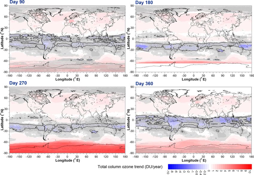
3886                                                     G. E. Bodeker et al.: A global total column ozone climate data record

2008). The database was first developed by NIWA (the New
Zealand National Institute of Water and Atmospheric Re-
search) and, in the last decade, has been maintained and up-
dated by Bodeker Scientific (BS). The non-filled database is
hereafter referred to as the NIWA-BS TCO database and the
filled database is referred to as the BS-filled TCO database.
The version 3.4 (V3.4) database reported on here extends
from 31 October 1978 to 31 December 2016. In construct-
ing this database, the guidelines for generating climate data
records of ECVs detailed in GCOS-143 (2010) have been ad-
hered to.
    Improvements over earlier versions of the database imple-
mented in V3.4 include the following:

    – New and updated sources of satellite-based TCO mea-
      surements are used, namely data from NPP-OMPS (Na-            Figure 1. A graphical representation of the different satellite-based
      tional Polar-orbiting Partnership-Ozone Mapping and           data sets used in this study and their periods of coverage. Satellites
      Profiler Suite), GOME-2 (Global Ozone Monitoring              marked with a dashed line indicate newly added source data for this
      Experiment-2), and SCIAMACHY (Scanning Imaging                version of the database.
      Absorption Spectrometer for Atmospheric CHartogra-
      phY) are now included in the combined data set. Vari-         1.25◦ × 1◦ resolution. The time periods covered by the satel-
      ous updates to previously used data sets are detailed in      lite data sets are shown graphically in Fig. 1.
      Sect. 2.                                                         In addition to the information presented in Table 1:
    – Improved statistical methods are used to model the dif-           – The four TOMS (Total Ozone Mapping Spectrometer)
      ference fields between data sets; zonal means of the dif-           data sets (Adeos, Earth Probe, Meteor 3, and Nimbus 7)
      ference fields are modelled using Legendre expansions               all use the TOMS retrieval algorithm with Adeos using
      which comprise the meridional component of a spheri-                the version 7 algorithm and the remaining three using
      cal harmonic expansion which is best suited for statisti-           the version 8 algorithm.
      cally describing a field on a sphere (see Sect. 3 for more
                                                                        – An algorithm similar to that used in the version 8 TOMS
      information).
                                                                          retrieval is used to conduct the version 8.6 retrievals of
                                                                          the SBUV (Solar Backscatter UltraViolet instrument)
    – Measurement uncertainties on the source data sets, and
                                                                          data (McPeters et al., 2013). Sparse gridded files were
      the corrections applied to those data sets, have been col-
                                                                          generated from the SBUV TCO measurements made at
      lated and are propagated through to the combined ozone
                                                                          discrete locations as input to the process that creates the
      data set so that, for the first time, this data set is now
                                                                          combined database.
      provided with uncertainty estimates for each datum.
                                                                        – The high-resolution and low-resolution OMI (Ozone
    – Furthermore, the gap-free BS-filled TCO database has                Monitoring Instrument) data sets both use a TOMS-like
      been generated (see Sect. 9) using a machine-learning               (version 8) retrieval algorithm.
      (ML) algorithm that is trained to capture the broad-
      scale morphology of the TCO field which extends to                – The GOME, GOME-2, and SCIAMACHY data sets all
      regions where measurements are missing. The ML al-                  use the GOME Direct Fitting (GODFIT) retrieval algo-
      gorithm is based on regression of available data against            rithm (Lerot et al., 2010).
      NCEP (National Centers for Environmental Prediction)              – As stated in Sect. 1.1 of the OMPS Algorithm Theo-
      CFSR (Climate Forecast System Reanalysis) reanalysis                retical Basis Document (ATBD), the algorithm used for
      tropopause height fields and against potential vorticity            retrieving the OMPS TCO is adapted from the heritage
      (PV) fields on the 550 K surface.                                   TOMS version 7 retrieval.

2    Source data                                                    3    Determining corrections to TOMS and OMI data

The various satellite-based TCO data sets used to create the        First, the corrections required to the TOMS and OMI data
version 3.4 NIWA-BS TCO database are summarized in Ta-              sets are determined by comparing the satellite-based mea-
ble 1. Where source data were provided at 1◦ × 1◦ resolu-           surements with TCO measurements made by the global Dob-
tion, bilinear interpolation was used to resample the data to       son spectrophotometer and Brewer spectrometer networks. A

Earth Syst. Sci. Data, 13, 3885–3906, 2021                                            https://doi.org/10.5194/essd-13-3885-2021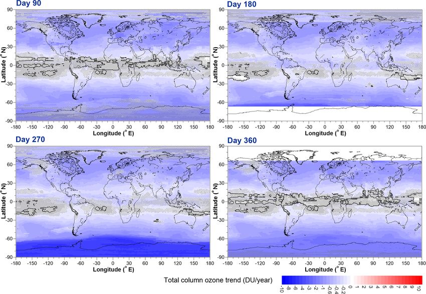
G. E. Bodeker et al.: A global total column ozone climate data record                                                         3887

Table 1. The source data sets used to create version 3.4 of the NIWA-BS TCO database.

   Data set                     Version    Period        Resolution (long × lat)
   TOMS/OMI
   Adeos                          7          1996–1997 1.25◦ × 1◦
   Source: https://data.ceda.ac.uk/badc/toms/data/adeos (last access: June 2021)
   Earth Probe                    8          1996–2005 1.25◦ × 1◦
   Source: https://data.ceda.ac.uk/badc/toms/data/earthprobe/ (last access: June 2021)
   Meteor-3                       8          1991–1994 1.25◦ × 1◦
   Source: https://data.ceda.ac.uk/badc/toms/data/meteor3 (last access: June 2021)
   Nimbus 7                       8          1978–1993 1.25◦ × 1◦
   Source: https://data.ceda.ac.uk/badc/toms/data/nimbus7 (last access: June 2021)
                                                            ◦
   Aura OMI, low resolution       8          2004–2012 1 × 1◦
   Source: https://disc.gsfc.nasa.gov/datasets/OMTO3e_003/summary (last access: June 2021)
   Aura OMI, high resolution 8               from 2004     0.25◦ × 0.25◦
   Source: https://disc.gsfc.nasa.gov/datasets/OMTO3e_003/summary (last access: June 2021)
   SBUV/SBUV2
   Nimbus 7                       8.6        1978–1990 overpass data
   Source: https://acdisc.gesdisc.eosdis.nasa.gov/data/Nimbus7_SBUV_Level2/SBUVN7O3.008/ (last access: June 2021)
   NOAA 9                         8.6        1985–1998 overpass data
   Source: https://acd-ext.gsfc.nasa.gov/anonftp/toms/sbuv/ (last access: June 2021)
   NOAA 11                        8.6        1988–2001 overpass data
   Source: https://acd-ext.gsfc.nasa.gov/anonftp/toms/sbuv/ (last access: June 2021)
   NOAA 16                        8.6        2000–2003 overpass data
   Source: https://acd-ext.gsfc.nasa.gov/anonftp/toms/sbuv/ (last access: June 2021)
   NOAA 14                        8.6        1995–2006 overpass data
   Source: https://acd-ext.gsfc.nasa.gov/anonftp/toms/sbuv/ (last access: June 2021)
   NOAA 17                        8.6        2002–2013 overpass data
   Source: https://acd-ext.gsfc.nasa.gov/anonftp/toms/sbuv/ (last access: June 2021)
   NOAA 18                        8.6        2005–2012 overpass data
   Source: https://acd-ext.gsfc.nasa.gov/anonftp/toms/sbuv/ (last access: June 2021)
   NOAA 19                        8.6        2009–2013 overpass data
   Source: https://acd-ext.gsfc.nasa.gov/anonftp/toms/sbuv/ (last access: June 2021)
   ESA
   GOME                            1.01      1996–2011 1◦ × 1◦
   Source: https://earth.esa.int/eogateway/instruments/gome (last access: June 2021)
   GOME-2                          1.00      2007–2012 1◦ × 1◦
   Source: https://www.eumetsat.int/gome-2 (last access: June 2021)
   SCIAMACHY                       1.00      2002–2012 1◦ × 1◦
   Source: https://www.sciamachy.org/products/index.php?species=O3 (last access: June 2021)
   Other
   NPP OMPS                       1.0        from 2012 1◦ × 1◦
   Source: https://disc.gsfc.nasa.gov/datasets/OMPS_NPP_NMTO3_L3_DAILY_2/summary?keywords=omps (last access: June 2021)

map showing the locations of the Dobson and Brewer sites is           Assumed uncertainties on the measurements from these two
available at https://woudc.org/data/stations/index.php?lang=          networks are presented below.
en (last access: June 2021). We assumed in all cases that                While TOMS and OMI data are provided in gridded data
the Dobson and Brewer spectrophotometer data submitted to             files, the original overpass data, unlike the gridded data set
the WOUDC (World Ozone and Ultraviolet Radiation Data                 where several measurements from different times through the
Centre) were the highest-quality data available, that all pos-        day might be averaged within a grid cell, provide location-
sible corrections to improve the quality of the data had been         specific measurements that are more suitable for comparison
made prior to submission, and that the measurements from              with the ground-based measurement networks; i.e. the over-
these two networks were unbiased with respect to each other.          pass measurements are specific to a latitude, longitude, and

https://doi.org/10.5194/essd-13-3885-2021                                               Earth Syst. Sci. Data, 13, 3885–3906, 2021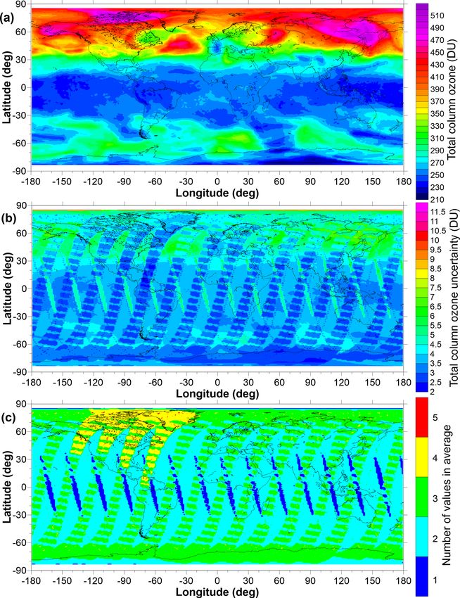
3888                                                     G. E. Bodeker et al.: A global total column ozone climate data record

date/time. To this end, overpass data from the four TOMS in-
struments and from the OMI instrument were obtained from
the GSFC (Goddard Space Flight Center) FTP server (https:
//disc.gsfc.nasa.gov/datasets, last access: July 2021). Dobson
and Brewer measurements were obtained from the WOUDC.
The 3-hourly means of the overpass data and direct-Sun Dob-
son and Brewer TCO measurements were calculated for all
sites for which Dobson and Brewer data were available. Ex-
clusion of some of the Dobson and Brewer data, as discussed
in Bodeker et al. (2001b), was required. Differences between
3-hourly means of ground-based and TOMS or OMI mea-
surements were calculated. The uncertainties on the differ-
ences were calculated as the root sum of the squares of the
uncertainties on the ground-based and satellite-based mea-
surements (see Sect. 5).
   The differences between the two data sets (satellite-based
and ground-based) can be described as an offset and a drift,        Figure 2. The results obtained by fitting Eq. (1) to the differ-
i.e.                                                                ences between Dobson/Brewer ground-based TCO measurements
                                                                    and Nimbus 7 TOMS overpass TCO measurements (ground-based
1(t) = α + βt,                                               (1)    minus satellite). Regions shaded in black denote the polar night
                                                                    where neither ground-based nor space-based measurements are pos-
where t is the time in decimal years, and α and β are fit coef-     sible. The thick black line denotes the zero contour. Differences are
ficients, denoting the offset and drift, respectively, to be de-    shown in Dobson units (DU; 1 DU = 2.69 × 10¹⁶ molecules cm−2 ).
termined through a regression model fit to the differences.
Because the offset and drift between the two data sets is
likely to depend on season and location, the α and β coef-          set (see below). The choice of NF,β = 0 is equivalent to there
ficients are expanded in a Fourier series to account for the        being no seasonal dependence in the drift. The resultant sta-
seasonality (see, e.g. Bodeker et al., 1998) and then further       tistically modelled difference field is a compromise between
expanded in spherical harmonics to account for the latitudi-        high accuracy and low complexity or, equivalently, a com-
nal and longitudinal structure in the difference field. Based       promise between simulating only meaningful structure in the
on theoretical expectations and past experience (Bodeker et         difference field and avoiding overfitting.
al., 2001b), we assume that the differences do not depend on           To avoid anomalous behaviour in the fit, which typically
longitude. Under this assumption, the spherical harmonic ex-        occurs at high latitudes and in regions where there are no
pansions reduce to Legendre polynomials. The α coefficient          satellite-/ground-based difference pairs (e.g. during the polar
then takes the form                                                 night), the region between 80◦ and the pole is populated with
                                                                    difference values of zero for 1 month on either side of the
     NX
      L,α −1                N
                             XF,α                                   winter solstice. An example of one such fit is shown in Fig. 2.
α=             Ll (θ ) αl0 +      αlf,sin sin(2πf t)                   The morphology of this Dobson/Brewer–Nimbus 7 TOMS
       l=0                   f =1                                   difference field is similar to that shown in Fig. 2 of Bodeker

                                                                    et al. (2001b) but with smaller differences resulting from
     + αlf,cos cos(2πf t) ,                                  (2)    the use of Legendre expansions in latitude, which better
                                                                    accommodate hemispheric asymmetries, rather than a trun-
where Ll denotes the lth Legendre polynomial and θ is the           cated polynomial expansion used in the earlier study. Sim-
co-latitude (90◦ − latitude). A similar expansion is made for       ilar 1(t, θ ) difference fields (not shown) were statistically
β. The choice of NL,α , NF,α , NL,β , and NF,β is somewhat          modelled for Adeos TOMS, Earth Probe TOMS, Meteor-3
arbitrary; the values need to be set sufficiently high to cap-      TOMS, and Aura OMI. Corrected TCO measurements for
ture the seasonal and latitudinal structure in α and β but not      each of these data sets were calculated as follows:
so high as to overfit the data and thereby introduce unreal-
istic structure into the statistically modelled difference field.   TCOcorr (t, θ, φ) = TCOuncorr (t, θ, φ) + 1(t, θ ),              (3)
Visual inspection of a wide variety of different choices of
NL,α , NF,α , NL,β , and NF,β led to choice of (4, 4, 3, 0) for     where φ is the longitude.
the statistical model of the TOMS and OMI difference fields
against the Dobson and Brewer networks where the Dobson             4   Determining corrections to all other data sets
and Brewer network is sparse, and (8, 4, 3, 0) for differences
from all other satellite-based data sources which are com-          The TOMS and OMI grids, corrected for their offsets and
pared against the more dense, corrected, TOMS/OMI data              drifts against the ground-based Dobson and Brewer mea-

Earth Syst. Sci. Data, 13, 3885–3906, 2021                                           https://doi.org/10.5194/essd-13-3885-2021
G. E. Bodeker et al.: A global total column ozone climate data record                                                              3889

                                                                       tion of the full data set. Because the combined TOMS/OMI
                                                                       record spans nearly the whole period (November 1978 to
                                                                       December 2016), extension into periods where TOMS/OMI
                                                                       data are not available is uncommon.
                                                                          In addition to deriving the corrections for each data set
                                                                       listed in Table 1, the uncertainties on each of these correc-
                                                                       tions were also calculated since they contribute to the uncer-
                                                                       tainties of the respective data set as discussed in Sect. 5. The
                                                                       overall uncertainties on each of the source data sets are used
                                                                       to create an uncertainty-weighted mean of all source data sets
                                                                       to produce the final TCO databases (see Sect. 6).

                                                                       5   Uncertainties on the source data sets

                                                                       One attribute of this version of the NIWA-BS TCO database
Figure 3. The results obtained by fitting Eq. (1) to the differences
                                                                       that differentiates it from previous versions is the provision
between corrected TOMS/OMI TCO zonal means and GOME TCO                of uncertainty estimates on each TCO value in the database.
zonal means. An additional basis function is included to account for   This development has been driven, in large part, by the re-
the 22 June 2003 anomaly. Regions shaded in black denote the polar     quirements for a climate data record as stipulated in GCOS-
night where space-based measurements in the UV–visible part of         143 (2010). Table 2 gives an overview of the literature on
the spectrum are not possible. The thick black line denotes the zero   which we have based the uncertainty estimates of our source
contour.                                                               data sets. For the NPP-OMPS instrument, the uncertainty on
                                                                       each TCO measurement comprises both a static component
                                                                       (in DU), and a component that scales with the TCO; i.e. it is a
surements, now form the basis to correct the other data sets           percentage of the TCO. The relevant values (1.12 DU for the
listed in Table 1. Differences between 1◦ zonal means from             static component and 0.64 % for the component that scales
the combined corrected TOMS/OMI data and from the re-                  with TCO) were derived from a linear fit to the data listed in
maining data sets are calculated individually for each data            Table 7.3-7 of Godin (2014).
set. The differences are then used as input to the regression             The random uncertainties on the raw values listed in Ta-
model described in Eq. (1). There could be a danger here that,         ble 2 are propagated through the analysis to result in an
in the case of biased longitudinal sampling by one satellite           uncertainty estimate on the final product. When regression
compared to another, the zonal means would be biased but               modelling the difference field between the ground-based
without these differences arising from any intrinsic biases            Dobson/Brewer measurements and the TOMS/OMI overpass
between the satellite-based measurements. Only the SBUV                TCO measurements, the uncertainties passed to the regres-
measurements were sparse and corrections for this potential            sion model (Eq. 1) are
sampling bias were derived as discussed below.
   If more than one TOMS/OMI meridional transect of zonal                        q
                                                                                      2 +σ2
means is available for a given day, then all available differ-         σdiff =       σDB  TOMS/OMI ovp ,                            (4)
ence values are passed to the regression model. As discussed
in Bodeker et al. (2005), on 22 June 2003, a tape recorder             where σDB is the measurement uncertainty on the Dob-
failure on the European Remote-Sensing 2 (ERS-2) satellite             son/Brewer measurements (1 %) and σTOMS/OMI ovp is the
resulted in only a small portion of the Northern Hemisphere            measurement uncertainty on the TOMS/OMI overpass mea-
being sampled by the GOME instrument thereafter. To ac-                surements.
count for possible discontinuities in the difference field intro-         The uncertainty on the modelled difference field is calcu-
duced by this anomaly, an additional basis function was in-            lated using a Monte Carlo approach, whereby the uncertain-
cluded in the regression model for the TOMS/OMI – GOME                 ties on each difference pair are used to generate new esti-
differences, set to 0 prior to 22 June 2003 and to 1 thereafter.       mates of the differences which then constitute a new data set
The resultant fit to the differences between zonal means of            of differences to which the statistical model is fitted. The pro-
TOMS/OMI and GOME is shown in Fig. 3.                                  cess is repeated 100 times. The mean and standard deviation
   The effects of the 22 June 2003 anomaly are clear in Fig. 3,        of the 100 resultant model fits provide the final difference
with higher and more variable differences after 22 June 2003           field and its uncertainty (σ1 ). The uncertainties on the cor-
than before. Statistically modelled difference fields, simi-           rected TOMS/OMI values, calculated using Eq. (3), are then
lar to that shown in Fig. 3, were generated for all non-               given by
TOMS/OMI data sets and extended, as required, to span the                                  q
temporal coverage of each of those data sets to permit correc-         σCorr (θ, φ, t) =       σuncorr (θ, φ, t)2 + σ1 (θ, t)2 .    (5)

https://doi.org/10.5194/essd-13-3885-2021                                                Earth Syst. Sci. Data, 13, 3885–3906, 2021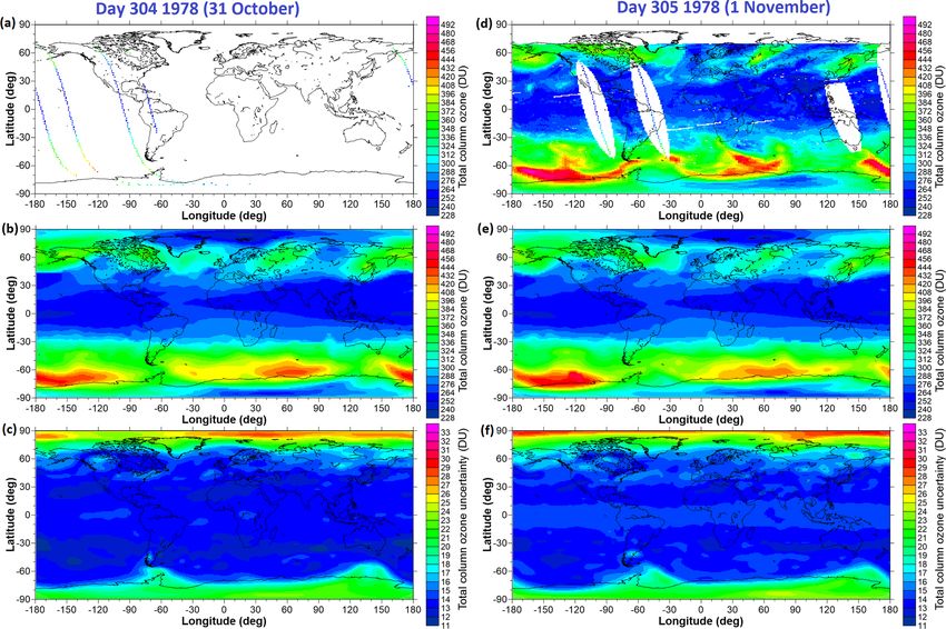
3890                                                        G. E. Bodeker et al.: A global total column ozone climate data record

Table 2. Typical uncertainties on the source data sets as reported in the references provided and as used in the construction of the TCO
databases. Note that the uncertainty on any particular measurement may differ from the typical values quoted in this table.

 Data set        Random error TCO         Source
 Dobson          1%                       Basher and Bojkov (1995): Survey of WMO-sponsored
                                          Dobson spectrophotometer intercomparisons
 Brewer          1%                       Fiolotev et al. (2005): The Brewer reference triad
 Adeos           2%                       Krueger et al. (1998): ADEOS TOMS data products user’s guide
 Earth Probe     2%                       McPeters et al. (1998): Earth Probe TOMS data products user’s guide
 Meteor-3        3%                       Herman et al. (1996): Meteor-3 TOMS data products user’s guide
 Nimbus 7        2%                       McPeters et al. (1996): Nimbus 7 TOMS data products user’s guide
 OMI             2%                       Bhartia (2002): OMI Algorithm Theoretical Basis Document Volume II, 2002
 All ESA         < 1.7 % (SZA < 80◦ )     GODFIT ATBD, 2013 (available at: https://climate.esa.int/en/projects/ozone/, last access: July 2021)
                 < 2.6 % (SZA > 80◦ )
 NPP OMPS        1.12 DU, 0.64 %          Godin (2014): OMPS NADIR TCO ATBD
 All SBUV        5.0 DU                   Pawan K. (PK) Bhartia (personal communication, 2014)

A similar procedure is used to propagate uncertainties in the
corrections of the other satellite data sets against the cor-
rected TOMS/OMI data sets. Recall that these corrections are
based on comparisons of zonal means. To estimate the uncer-
tainties on the zonal means, rather than taking the weighted
mean of the single measurements, the unweighted arithmetic
mean is calculated so that every measurement has the same
weight. The zonal mean (ZM) and its uncertainty (σZM ) are
then given by
                              v
           N
                              uN
        1 X                1u    X
ZM =          xi    σZM = t          σi2 ,                (6)
        N i                N      i

where N is the number of measurements in the zone, xi indi-
cates the measurements, and σi indicates the uncertainties on            Figure 4. The additional uncertainty introduced to the SBUV zonal
the measurements. The uncertainty on the zonal mean also                 means as a result of undersampling the zonal TCO profile. Regions
                                                                         shaded in white denote the polar night where space-based measure-
needs to account for the effects of any undersampling. If the
                                                                         ments in the UV–visible part of the spectrum are not possible.
zonal profile of TCO is highly structured, perhaps as a result
of planetary-scale waves, then, if a particular space-based in-
strument does not fully capture that structure, the uncertainty
on the zonal mean will be higher than would have been the                talling 21 d. This gives a sample data set of 210 data grids.
case otherwise. This is primarily a concern for the sparse               For each SBUV data set available on that calendar day, and
sampling by the SBUV instruments used to create the com-                 for each latitude, two zonal means are calculated, namely (1)
bined database. For the SBUV data sets, in addition to the               the true zonal mean (ZMtrue ) calculated from the 1440 values
zonal mean uncertainty calculated using Eq. (6), the poten-              comprising the zonal TCO profile at 0.25◦ resolution, and (2)
tial uncertainty resulting from the sparse sampling was also             the subsampled zonal mean (ZMsub ) calculated using only
accounted for. To estimate this additional uncertainty in the            those OMI data at the locations of the SBUV measurements.
zonal means calculated using SBUV measurements, an algo-                 For each latitude, 210 (from the 21 d window of 10 years
rithm was developed to compare the zonal mean of a well-                 of OMI data used) difference pairs of ZMtrue − ZMsub can
sampled zonal TCO profile with the zonal mean calculated                 be calculated. If the SBUV sampling of the zonal mean was
using the same zonal profile but sampled at the SBUV mea-                unbiased, all 210 values would be 0.0. The mean and stan-
surement locations. The high-spatial-resolution (0.25◦ ) OMI             dard deviation of these 210 values are then calculated, and
data set was used for this purpose. To estimate the poten-               the standard deviation is used as an estimate of the SBUV
tial zonal mean uncertainty for each day of the year result-             subsampling uncertainty (σsubsample ) which is specific to a
ing from the SBUV undersampling, grids of high-spatial-                  particular SBUV instrument and depends on the year and lat-
resolution data from OMI were considered for 10 years (2004              itude. An example of one such subsampling uncertainty field
to 2013) and for 10 d before and after the day of interest, to-          for the NOAA 19 SBUV instrument is shown in Fig. 4.

Earth Syst. Sci. Data, 13, 3885–3906, 2021                                                https://doi.org/10.5194/essd-13-3885-2021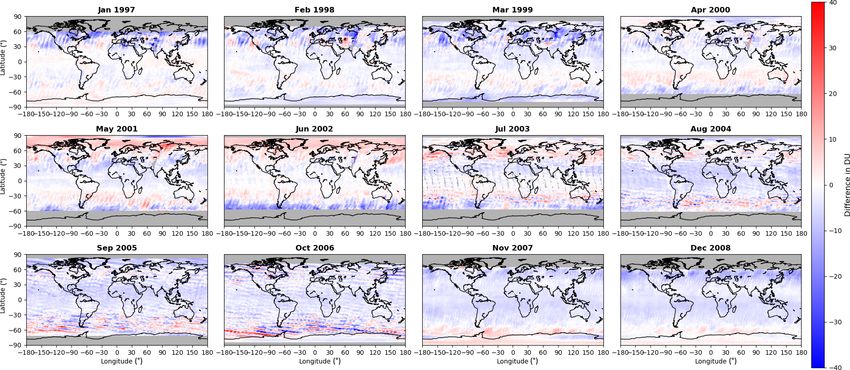
G. E. Bodeker et al.: A global total column ozone climate data record                                                           3891

   The subsampling uncertainty maximizes during periods
when the zonal profile shows more complex structure, i.e.
typically in winter and spring when midlatitude planetary
wave activity maximizes. The subsampling uncertainty on
the zonal means is added to the zonal mean uncertainty cal-
culated using Eq. (6) as
            q
σZMSBUV = σZM  2 +σ2                                    (7)
                      subsample .

6   Creating the combined data set

To construct a single TCO field for each day, a weighted
mean of all available corrected measurements in each grid
cell is calculated. A grid of 1.25◦ longitude by 1.0◦ latitude
was selected for the final product. The weights applied to the
individual available TCO measurements are derived from the
measurement uncertainties on each available measurement,
namely
            P
                wi,j,k TCOi,j,k
TCOi,j = k P
                    k wi,j,k
            P 2          2
  2           k wi,j,k σi,j,k
σTCO      = P                 ,                             (8)
      i,j    ( k wi,j,k )2

where i and j are indices over latitude and longitude, k is
an index over the measurements from different satellites in
that cell, and the weights (wi,j,k ) are calculated as 1/σ 2 ,    Figure 5. Example fields for 21 March 2005: (a) the TCO field,
where σ is the measurement uncertainty incorporating any          (b) the uncertainties on each value plotted in panel (a), and (c) the
                                                                  number of values averaged to create the means plotted in panel (a).
additional uncertainty introduced by corrections made to the
                                                                  Regions shaded in white denote the polar night where space-based
original data. Unlike previous versions of this TCO database,     measurements in the UV–visible part of the spectrum are not possi-
the daily combined TCO fields are accompanied by fields of        ble.
uncertainties and fields detailing the number of values that
were averaged to produce the single combined value. An ex-
ample of these three fields for one selected day is given in      section were calculated by subtracting the validation values
Fig. 5.                                                           from the NIWA-BS values such that positive differences rep-
   As expected, Fig. 5 shows that the uncertainty on TCO          resent elevated ozone values in the NIWA-BS database com-
values decreases with an increasing number of source data         pared to the validation databases. Figure 6 shows the globally
sets. The regions of elevated uncertainty, sloping from north-    averaged area-weighted differences between the NIWA-BS
west to south-east across the Equator, arise from having only     database and the validation databases over the full time pe-
the OMI TCO values available to build the mean. Cyan re-          riod.
gions in Fig. 5c show where additional Earth Probe TOMS              The NIWA-BS database displays a small negative bias
data contribute (with a resultant reduction in the uncertainty)   (−0.2 ± 2.7 DU) against the global mean monthly means
and regions in green where SCIAMACHY additionally con-            calculated from the Dobson and Brewer measurements ob-
tributes data, reducing the uncertainties in the resultant mean   tained from the WOUDC. A slightly larger negative bias
to less than 3 DU.                                                (−1.2 ± 1.2 DU) is seen in comparison with the SBUV V8.6
                                                                  NASA time series. The bias against the SBUV V8.6 data set
7   Validating the combined data set                              produced by NOAA is slightly more negative but not statisti-
                                                                  cally significantly different from zero (−1.3 ± 1.5 DU). The
This new NIWA-BS TCO database has been validated                  comparison against the GSG Bremen database suggests that
through comparisons with the WOUDC database and four              the NIWA-BS time series exhibits a small anomalous down-
additional independent TCO databases listed in Table 3.           ward trend starting around 2002, which is also reflected in
To account for different spatial resolutions, the NIWA-BS         the WOUDC comparison and in the ESA CCI comparison.
database was regridded to match the spatial resolution of            Seasonal mean differences between the NIWA-BS
each validation database. The differences reported in this        database and the five validation databases, as a function of

https://doi.org/10.5194/essd-13-3885-2021                                         Earth Syst. Sci. Data, 13, 3885–3906, 2021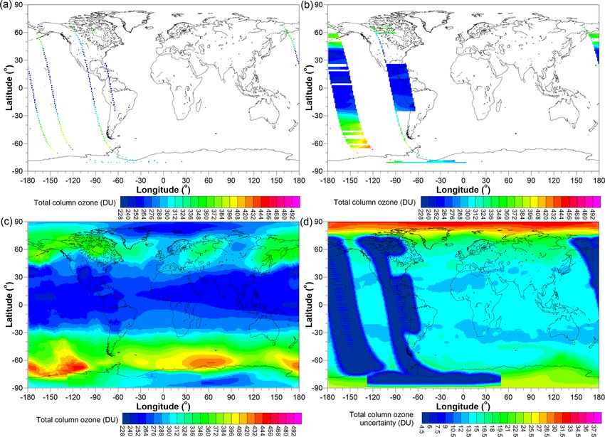
3892                                                        G. E. Bodeker et al.: A global total column ozone climate data record

Table 3. Sources and details of the independent data sets used to validate the NIWA-BS total column ozone database.

          Data set               Instruments                 Record length              Reference
          SBUV V8.6 NASA          BUV Nimbus 4,             May 1970 to Dec 2017 McPeters et al. (2013); Frith et al. (2014)
                                  SBUV Nimbus 7,
                                  SBUV/2 NOAA 9 to 19
          Source: https://acd-ext.gsfc.nasa.gov/Data_services/merged/ (last access: June 2021)
          SBUV V8.6 NOAA          SBUV Nimbus 7,            Nov 1978 to Dec 2015 Wild et al. (2012); McPeters et al. (2013)
                                  SBUV/2 NOAA 9 to 19
          Source: https://acd-ext.gsfc.nasa.gov/Data_services/merged/instruments.html (last access: June 2021)
          GSG Bremen            GOME,                   Jul 1995 to Dec 2016       Weber et al. (2013)
                                SCIAMACHY,
                                GOME-2
          Source: https://www.iup.uni-bremen.de/gome/wfdoas/ (last access: June 2021)
          ESA CCI                 GOME,                        Mar 1996 to Jun 2011     Lerot et al. (2014)
                                  SCIAMACHY,
                                  GOME-2
          Source: https://climate.esa.int/en/projects/ozone/ (last access: June 2021)

latitude, are shown in Fig. 7. In general, the differences               an underestimation of TCO in the northern subtropics during
between the NIWA-BS TCO database and the validation                      the first half of each year and underestimations just equator-
databases are smaller than the uncertainties in the NIWA-BS              ward of the polar night in the Southern Hemisphere.
database. This is not the case, however, in the high northern               As the NOAA SBUV database is available at daily reso-
latitudes in winter where the NIWA-BS database shows sta-                lution as for the NIWA-BS TCO database, daily differences
tistically significantly smaller ozone values compared to the            between zonal means from these two databases are calculated
validation data sets. This results from larger differences in            and shown in Fig. 10.
satellite measurements and ground-based measurements be-                    Over their full overlap period, the average difference is
ing inferred close to the region of permanent polar darkness             −1.44 DU, with 95 % of the differences between −8.66 and
where both satellite and ground-based measurements are                   5.35 DU. Similar to the NASA SBUV comparisons, there ap-
scarce; i.e. there were only 548 Dobson/Brewer–satellite dif-            pears to be a small underestimation in TCO over the northern
ference pairs in the winter (DJF) Arctic (poleward of 60◦ N)             subtropics in the first half of many years.
on which to base the correction.                                            Differences between monthly mean 5◦ zonal mean TCO
   A more in-depth comparison of the NIWA-BS database                    from the NIWA-BS database and the GSG Bremen TCO data
and the WOUDC database is presented in Fig. 8, where                     set which combined GOME, SCIAMACHY, and GOME-2
monthly mean zonal means (in 5◦ latitude zones) are dif-                 data are shown in Fig. 11.
ferenced (NIWA-BS minus WOUDC). Over their full pe-                         There appears to be a consistent underestimation of TCO
riod of overlap, the mean difference between the data sets               in the NIWA-BS database equatorward of the polar night
is −0.26 DU, with 95 % of the differences falling between                from January to March in most years with respect to GSG
−11.38 and 13.21 DU. Differences between the data sets are               Bremen. The mean difference between the databases is
larger at higher latitudes. A consistent feature of the NIWA-            −3.14 DU, with 95 % of the differences lying between −9.79
BS TCO database across most years is an overestimation in                and 2.81 DU.
TCO equatorward of the Antarctic and an underestimation of                  Validation data from the ESA Climate Change Initiative
TCO close to the South Pole with respect to WOUDC.                       (CCI) level 3 TCO data set are available as monthly mean
   Differences between monthly mean 5◦ zonal means from                  maps, and differences between these monthly mean maps and
the NIWA-BS database and NASA SBUV merged ozone                          NIWA-BS TCO are shown in Fig. 12.
database version 8.6 are shown in Fig. 9.                                   While there is significant spatial structure in some of
   The mean difference in TCO across the full overlap period             the monthly difference fields, there is little structure that
is −1.21 DU, with 95 % of the differences in the range −5.96             is consistent across multiple years. The mean difference
to 2.95 DU. The differences are smaller in magnitude than                is −2.36 DU, with 95 % of the differences lying between
those shown in Fig. 8 and show smaller year-to-year vari-                −10.63 and 6.34 DU.
ability, perhaps as a result of the more dense spatiotemporal
sampling by the SBUV instruments compared to the ground-
based instruments. Features common across most years are

Earth Syst. Sci. Data, 13, 3885–3906, 2021                                                https://doi.org/10.5194/essd-13-3885-2021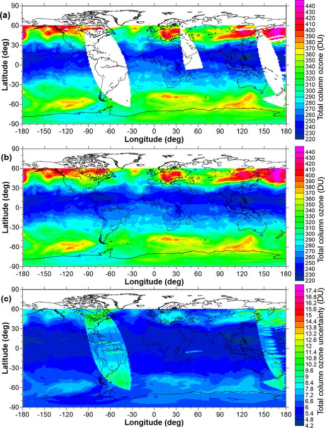
G. E. Bodeker et al.: A global total column ozone climate data record                                                          3893

Figure 6. Area-weighted global mean monthly mean differences in TCO between the NIWA-BS database and the validation databases
detailed in Table 3. The topmost panel shows the differences between the NIWA-BS database and the ground-based TCO database obtained
from the WOUDC. The remaining four panels show differences against databases derived from space-based measurements. The statistics in
the top right corner of each panel show the mean difference and standard deviation.

8   Calculation of monthly mean and annual mean
    fields                                                             2
                                                                     σi,new = σi2 + (xi − xi,exp )2 ,                            (9)
Monthly mean TCO fields at 1.25◦ longitude and 1◦ lati-              where xi,exp is the “expectation” value which is taken to be
tude resolution (the same resolution as the daily fields) have       the unweighted mean of the available measurements. The
been calculated, together with their uncertainties. The algo-        mean is then calculated as
rithm was used to calculate the mean and its uncertainty from             PN
N measurements (xi , i = 1, . . ., N ). The uncertainty on the              i=1 wi,new × xi
                                                                     x= P      N
                                                                                            ,                                (10)
mean is calculated in such a way that it depends on both the                   i=1 wi,new
uncertainties on the measurements (σi ) and on the variance                               2
in the measurements. First, a revised uncertainty for each da-       where wi,new = 1/σi,new  and the uncertainty is calculated as
tum is calculated to reflect the true confidence we have on               v
                                                                          u PN 2
each measurement as an estimator of the mean:                                    i=1 σi,new × wi
                                                                          u
                                                                     σx = t                        ,                          (11)
                                                                            (NF − 1) × N
                                                                                          P
                                                                                            i=1 wi

https://doi.org/10.5194/essd-13-3885-2021                                            Earth Syst. Sci. Data, 13, 3885–3906, 2021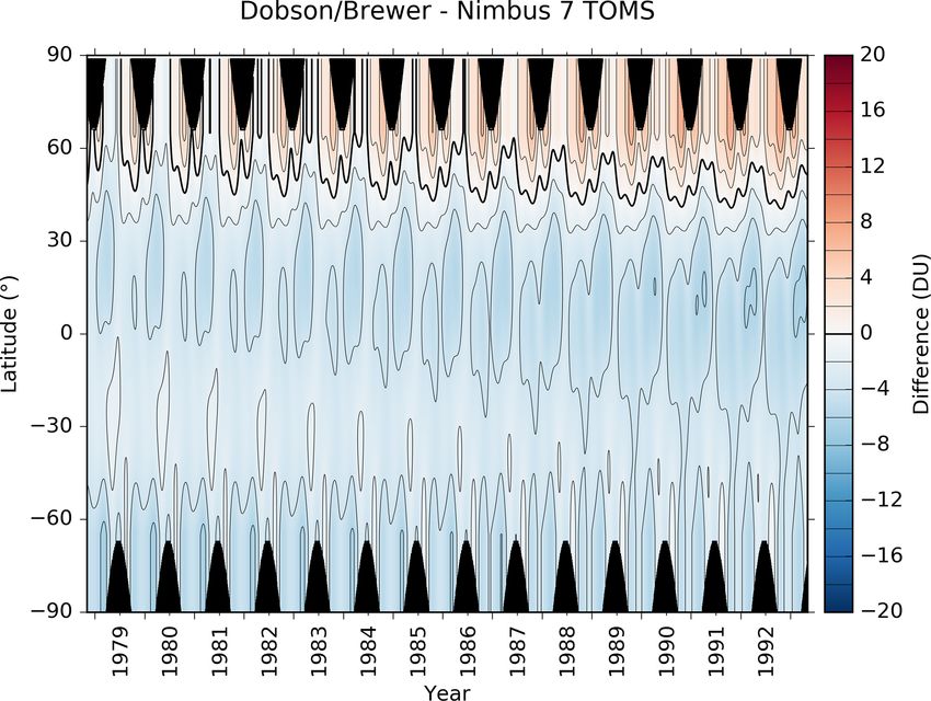
3894                                                    G. E. Bodeker et al.: A global total column ozone climate data record

Figure 7. TCO differences (NIWA-BS TCO minus validation database) as a function of latitude plotted as seasonal means over the entire
period of data available. The 1σ uncertainty range in the NIWA-BS TCO is shown in black and the standard deviation on the differences
between NIWA-BS TCO and each validation database is shown by the shading.

Figure 8. Monthly mean differences between NIWA-BS TCO and the WOUDC database for 12 selected years.

Earth Syst. Sci. Data, 13, 3885–3906, 2021                                           https://doi.org/10.5194/essd-13-3885-2021
G. E. Bodeker et al.: A global total column ozone climate data record                                                         3895

Figure 9. Differences between monthly mean zonal means calculated from the NIWA-BS TCO database and the NASA SBUV V8.6 database
(NIWA-BS minus SBUV) for 12 selected years.

where wi = 1/σi2 and NF is the degrees of freedom. In this            The result is a TCO field that replicates the original data
case, NF was taken to be N − 1 to account, in part, for            where they are available and, where no data are available,
auto-correlation in the daily time series used to calculate the    transitions preferentially into the conservatively filled field
monthly and annual means. The monthly mean and annual              (Field 1). Where the conservatively filled field has missing
mean TCO fields are provided as a component of the version         data, we transition into the ML-filled field (Field 2). Each
3.4 database.                                                      “transition” is achieved by way of the blending process de-
                                                                   scribed below.
9    Creating the BS-filled total column ozone
     database
                                                                   9.1   The conservatively filled field – Field 1
For some applications, there is a need for gap-free TCO
fields, e.g. TCO fields for validating chemistry-climate mod-      First, a spatial nearest-neighbour interpolation is used to fill
els which generate TCO fields over the entire globe for each       as many missing values as possible. This is done by searching
day of the year. To create a filled TCO database for a tar-        for cells with null TCO values that are neighboured, either to
get day, the following steps are performed, each of which is       the north and south, or to the east and west, by non-null val-
detailed in subsections below.                                     ues. If such a non-null pair is found, that pair of TCO values,
    1. A conservatively partially filled field is created (here-   together with their uncertainties, is used to estimate the inter-
       after referred to as Field 1).                              stitial value which is taken as the mean of the two neighbour-
                                                                   ing values. Preference is given to zonal nearest neighbours.
    2. A ML method is used to create a best estimate of the        The uncertainty on the interpolated values is calculated by
       completely filled TCO field for the target day (hereafter   adding in quadrature the uncertainties on the neighbouring
       referred to as Field 2).                                    values.
                                                                      After doing the spatial nearest-neighbour interpolation,
    3. The original unfilled TCO field, Field 1, and Field 2 are   cases are sought where, for a cell containing a null value on
       then “blended” (using an algorithm described below) to      day N, there are non-null values in the same cell on day N −1
       generate the final filled field.                            and day N +1. Temporal nearest-neighbour interpolation be-
                                                                   tween the previous and following day is done in the same

https://doi.org/10.5194/essd-13-3885-2021                                         Earth Syst. Sci. Data, 13, 3885–3906, 2021
3896 G. E. Bodeker et al.: A global total column ozone climate data record
Figure 10. Daily differences between 5◦ zonal means calculated from the NIWA-BS TCO database and the NOAA SBUV V8.6 database
for the same years as in Fig. 9.
way as described for the spatial nearest-neighbour interpola- 9.2 The machine-learning-estimated field – Field 2
tion.
To create a completely filled TCO field for each day, a regres-
Following the spatial–temporal nearest-neighbour interpo-
sion model, including an offset basis function, a tropopause
lation, a more extensive longitudinal interpolation finds two
height basis function, and a potential vorticity at 550 K basis
non-null values at the same latitude that are separated by two
function, is trained on a “window” of data around the target
or more null values with the constraint that the non-null val-
date. The trained regression model is used to generate a filled
ues cannot be separated by more than 30◦ in longitude. Lin-
TCO field on the target date.
ear interpolation between the two non-null values, including
The regression model is of the form
an estimate of the uncertainties, is used to determine the in-
terstitial values and their uncertainties. The spatial–temporal
TCOi,j = α(θ, φ) + β(θ, φ) × THi,j
nearest-neighbour interpolation, and the longitudinal inter-
polation, are repeated until no additional values are inserted + γ (θ, φ) × PV550i,j + Ri,j , (12)
into the grid. The result is a conservatively interpolated TCO
where i, j subscripts denote indices over latitude (θ) and lon-
field, still containing missing values, together with its origi-
gitude (φ), TH and PV550 are 6-hourly tropopause height
nal uncertainty field and traceable uncertainties on the newly
fields and 500 K potential vorticity fields, respectively, ob-
interpolated values. A plot of the original TCO field, the con-
tained from NCEP CFSR (National Centers for Environ-
servatively filled field, and the uncertainties on the conserva-
mental Prediction) CFSR (Climate Forecast System Re-
tively filled field for day 3 of 1980 are shown in Fig. 13.
analysis) reanalyses prior to 31 December 2010, and from
The structure in the uncertainty field results from the prop-
NCEPCFSv2 reanalyses thereafter (Saha et al., 2010). α, β,
agation of uncertainties when calculating the conservatively
and γ are fit coefficients and Ri,j are the residuals that re-
filled field – larger uncertainties result when interpolated val-
main due to variance that cannot be explained by the regres-
ues are spatially far from available measurements.
sion model.
Earth Syst. Sci. Data, 13, 3885–3906, 2021 https://doi.org/10.5194/essd-13-3885-2021G. E. Bodeker et al.: A global total column ozone climate data record 3897 Figure 11. Differences between monthly mean 5◦ zonal mean TCO calculated from the NIWA-BS and GSG Bremen databases for 12 selected years (NIWA-BS minus GSG). Figure 12. Differences between monthly mean TCO fields calculated from the NIWA-BS database and those available from the ESA CCI database for 12 selected months/years. https://doi.org/10.5194/essd-13-3885-2021 Earth Syst. Sci. Data, 13, 3885–3906, 2021
3898 G. E. Bodeker et al.: A global total column ozone climate data record
The Ylm can be expressed as
0 if m = 0
Y
√l ,
m m
Yl = 2N(l,m) Pl (cos θ ) cos(m × φ), if m > 0 (14)
√
2N(l,m) Pl−m (cos θ ) sin(m × φ) if m < 0.
For the purposes of fitting √ Eq. (14) to the TCO fields, the
normalization constants ( 2N(l,m) ) can be ignored as they
are taken up into the fit coefficients. When fitting Eq. (12),
the initial N value for α is set as 10 and for β and γ as 2.
The maximum allowed N value for α is 10 and for β and
γ is 5. The initial l 0 value for α was set at 5 (with a maxi-
mum allowed value of 5) and for β and γ as 2 (with max-
imum allowed values of 5). These initial values and limits
on the spherical harmonics expansions were selected based
on careful consideration of the scales of spatial structures in
TCO fields, and on how the dependence of TCO on TH and
PV550K varies spatially. The training of the algorithm hap-
pens “around” the target date as fields on neighbouring dates
and years are used to establish the dependence of TCO on
TH and PV550K. A search ellipse, initially extending 3 d on
either side of the target date, and 1 year on either side of
the target date, is defined to select TCO fields for the train-
ing where the ellipse is iteratively expanded until there are
20 TCO fields available for the training. The extension to
neighbouring years is done because, in some cases, there are
missing TCO fields in the current year such that a reliable fit
Figure 13. (a) The original unfilled TCO field on 3 January 1980, of Eq. (12) cannot be performed. Within this search ellipse,
(b) the conservatively filled TCO field on the same day, and (c) the the dependence of TCO on TH and PV550K at a similar time
uncertainties on the conservatively filled field. White regions show of the year is expected to hold.
where data are missing. From these 20 TCO fields, to avoid excessive computa-
tional expense, only up to 20 000 data points are passed to
the regression model by sampling every lth value from all
As denoted in Eq. (12), the three fit coefficients depend on
data available for training such that the total number of val-
latitude and longitude. That dependence is captured by ex-
ues passed is less than or equal to 20 000. The latitude and
panding the fit coefficients in spherical harmonics in a similar
longitude of each ozone value is also passed to the regres-
way as was done in Eq. (2), i.e.
sion model so that the associated TH and PV550K values can
l0
N X
be extracted. The times associated with the TCO fields are
assumed to be local noon times (since most of the satellites
X
α(θ, φ) = αlm Ylm (θ, φ), (13)
l=0 m=−l 0 making the underlying measurements were Sun-synchronous
satellites with an Equator-crossing time close to solar noon).
where Therefore, the actual UTC time varies across the TCO field.
The TH and PV550K values are linearly interpolated to those
– θ is the co-latitude, exact UTC times.
Various “versions” of the regression model are tested; i.e.
– φ is the longitude, different basis functions are excluded/included; the offset (α)
basis function is always included. In addition to switching
– N is a regression model parameter,
different basis functions on/off, different values for N and l 0
– l 0 ≤ l where the exact limit for l 0 is also a regression are tested (perturbing these by ±1 around their start value)
model parameter, but ensuring that the maximum allowed zonal and merid-
ional expansions are not exceeded (see above). This results
– αlm indicates the fit coefficients, and in many different possible constructs of the regression model.
If any model, when evaluated over every latitude and longi-
– Ylm (θ, φ) is the spherical harmonic function of degree l tude, results in a TCO value more than 10 % above the max-
and order m. imum measured TCO value passed to the regression model,
Earth Syst. Sci. Data, 13, 3885–3906, 2021 https://doi.org/10.5194/essd-13-3885-2021G. E. Bodeker et al.: A global total column ozone climate data record 3899
or below 10 % less than the minimum value passed to the re- where C is the blended value, W is a weight calculated as de-
gression model, it is discarded to eliminate statistical models tailed below, Aproxy is a proxy value for the missing value in
that significantly overfit the TCO field. In addition to hav- Field A determined as detailed below, and Bvalue is the non-
ing a model with an excess of fit coefficients, overfitting can null value from Field B. To derive an Aproxy value, a box of
also occur when anomalous values in the TH or PV550 fields size 41 × 41 cells is centred on the missing value and divided
result in excessively high or low TCO values being gener- into six sectors each subtending an angle of 60◦ . Each sec-
ated. This is why models that exclude/include these two ba- tor is scanned for non-null values in Field A, and a weighted
sis functions are also tested. For all models that pass this ini- mean of those six values is calculated these weights:
tial test, a Bayesian information criterion (BIC; Liddle, 2007)
score is calculated as D×π
Wi = cos , (17)
2 × 10⁶
BIC = M × ln(R 2 /M) + NC × ln(M), (15)
where D is the distance to the nearest non-null value in that
where M is the number of data passed to the regression
sector measured in metres. The weight is set to zero when
model, R 2 is a modified sum of the squares of the residu-
D is greater than 1000 km. Aproxy is then set to the weighted
als, and NC is the total number of coefficients in the fit. R 2
mean of the non-null values across all six sectors.
is modified to provide a strong disincentive for models gen-
In calculating the blended value using Eq. (16), the weight
erating values outside the range of measurements, i.e. where
(W ) is calculated using the distance to the nearest non-null
model values are below the minimum or above the maximum
value across all six search sectors in Eq. (17). If no Aproxy
measurement passed to the regression model, the residual is
value can be found, then W in Eq. (16) is set to zero. Standard
inflated exponentially to impose an additional cost on the
error propagation rules are used to determine an uncertainty
model for generating values outside of the range of the data.
on the blended value. This process results in using values
Typically, for each daily TCO field, several hundred fits
from Field A where they are available which then blend into
of the regression model are performed to find the optimal
values from Field B when they are not available.
model construct (minimum BIC). This optimal model is then
used to generate the statistically modelled TCO field. The
database of different regression models is also used to cal- 9.4 Blending the original unfilled TCO field, Field 1, and
culate the structural uncertainties that result from different Field 2 to construct the final filled field
possible choices of spherical harmonic expansions. The un- For each day, the original TCO field, the conservatively filled
certainties that result from uncertainties on the regression field (Field 1), and the ML-modelled field (Field 2) are
model fit coefficients are also calculated. These two sources merged in such a way that the original values are preserved
of uncertainty are then added in quadrature. The structural where they are available. Where they are not available, the
uncertainty statistics are calculated using only those regres- filled values relax to the conservatively filled field where they
sion modelled fields (out of the several hundred) that have the are available. Where conservatively filled values are also not
same sequence of basis functions switched on and off com- available, the filled values relax to the ML-modelled field.
pared to the best fit. Examples of the unfilled TCO fields, the The ML-modelled fields, because they are modelled on
ML-modelled TCO fields, and the uncertainty on the mod- PV550K and TH (which themselves can contain anomalous
elled TCO fields for days 304 and 305 of 1978 are shown in values), can occasionally display physically unrealistic spa-
Fig. 14. tial or temporal structures so, for any given day, to obtain
a smoother ML-filled field, a (1, 4, 6, 4, 1) weighting of the
9.3 An algorithm for blending a primary and secondary five daily ML-filled fields, centred on the day of interest, is
TCO field calculated.
For the final blended data product, several possibilities ex-
This section describes an algorithm to “blend” some pri-
ist for any given day, i.e.
mary TCO field (hereafter Field A) with some secondary
field (hereafter Field B) to create a single blended field (here- – None of the three fields are available: in this case, no
after Field C), where the Field A values are preserved while final filled field is generated.
smoothly transitioning to the Field B values. This algorithm
is used below to combine the original TCO field and Field 1, – Only the ML-modelled field is available: in this case,
and/or to combine Field 1 and Field 2, and/or to combine the the ML-modelled field (possibly spatially smoothed)
original TCO field and Field 2; see Sect. 9.4. and its associated uncertainties become the final filled
If there is a null value in a cell in Field A and a non-null field for the target day.
value in the same cell in Field B, then a proxy value for Field
– Only the conservatively filled field and the ML-
A is found and combined with the value from Field B as fol-
modelled fields are available: in this case, the conser-
lows:
vatively filled field (Field 1) and the ML-modelled field
C = W × Aproxy + (1 − W ) × Bvalue , (16) (Field 2) are blended to create the final filled field.
https://doi.org/10.5194/essd-13-3885-2021 Earth Syst. Sci. Data, 13, 3885–3906, 20213900 G. E. Bodeker et al.: A global total column ozone climate data record
Figure 14. (a, d) The original unfilled TCO fields on 31 October and 1 November 1978, respectively; (b, e) the machine-learning-modelled
fields; (c, f) the uncertainties associated with the machine-learning-modelled fields. On 31 October, the optimal fit was obtained by expanding
the offset basis function in spherical harmonics of degree 10 and order 5, expanding the tropopause height basis function in spherical
harmonics of degree 4 and order 3, and the PV at 550 K basis function in spherical harmonics of degree 5 and order 3. For 1 November, these
expansions were (10, 5) for the offset basis function (4, 3) for the TH basis function and (5, 4) for the PV550K basis function.
– All three fields are available: in this case, the conserva-
tively filled field and the ML-modelled field are blended
to create an intermediate field. The original TCO field Ozone(m, θ, φ) = A(m, θ, φ)
and the intermediate field are then blended to create the [max Fourier] = 4
final filled TCO field and its uncertainty. + B(m, θ, φ) × m/12
[max Fourier = 3]
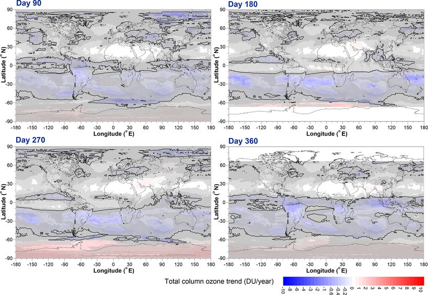
An example of the original field for TCO on 31 October + C(m, θ, φ) × mm=0 if yearG. E. Bodeker et al.: A global total column ozone climate data record 3901 Figure 15. (a) The original unfilled TCO field on 31 October 1978, (b) the conservatively filled field, (c) the final filled field, and (d) the uncertainties on the final filled field. where Ozone(m, θ, φ) is the regression modelled TCO in trend over the full period, while the C coefficients diagnose month m (m = 1 to NY×12, where NY is the total number of the change in trend from 2000 onward. The year from 1999 to years of data) and at latitude θ and longitude φ. The monthly 2000 was prescribed as the trend transition year, as this is ap- mean TCO values were calculated as detailed in Eq. (10) and proximately when stratospheric chlorine and bromine load- Eq. (11). Equation (18) is fitted independently to the monthly ing peaked (Newman et al., 2007). We also wanted to ensure mean time series at each latitude and longitude. A to I are that the first trend period included data from the late 1990s as the regression model coefficients calculated using a standard there was a greater likelihood of missing data from 1994 to least squares regression (Press et al., 1989). 1998, and we wanted to avoid end-effect biasing in the calcu- The first term in the regression model (A coefficient) rep- lation of the trends. That said, the conclusions drawn below resents a constant offset and, when expanded in a Fourier regarding changes in trend were found to be largely insen- series, represents the mean annual cycle. In addition to the sitive to the selection of the transition year within 2 years offset coefficient, each fit coefficient can depend on season; of the selected transition year. The quasi-biennial oscillation e.g. TCO trends vary with season. Therefore, each coeffi- (QBO) basis function was specified as the monthly mean cient is expanded in Fourier pairs, as explained in Sect. 2.2 of 50 hPa Singapore zonal wind. The phase of the QBO varies Bodeker and Kremser (2015). The actual number of Fourier with latitude and, to permit fitting of the phase, a second pairs for each regression coefficient is determined by finding QBO basis function, mathematically orthogonalized to the the optimal set of expansions across all fit coefficients that first, was included in the regression model as was done in minimizes a BIC as described above. The maximum number Bodeker et al. (2013). of Fourier pairs permitted for each regression model coeffi- The El Niño–Southern Oscillation (ENSO), solar cycle, cient is listed in Eq. (18). The B coefficients diagnose the Mt. Pinatubo, and El Chichón basis functions were the same https://doi.org/10.5194/essd-13-3885-2021 Earth Syst. Sci. Data, 13, 3885–3906, 2021
You can also read