Topology and obliquity of core magnetic fields in shaping seismic properties of slowly rotating evolved stars
←
→
Page content transcription
If your browser does not render page correctly, please read the page content below
MNRAS 504, 3711–3729 (2021)                                                                                                     doi:10.1093/mnras/stab991
Advance Access publication 2021 April 14

Topology and obliquity of core magnetic fields in shaping seismic
properties of slowly rotating evolved stars
                              ‹
Shyeh Tjing Loi
Department of Applied Mathematics and Theoretical Physics, University of Cambridge, Centre for Mathematical Sciences, Wilberforce Road, Cambridge CB3
0WA, UK

Accepted 2021 April 6. Received 2021 April 6; in original form 2020 December 18

                                                                                                                                                             Downloaded from https://academic.oup.com/mnras/article/504/3/3711/6225807 by guest on 18 September 2021
ABSTRACT
It is thought that magnetic fields must be present in the interiors of stars to resolve certain discrepancies between theory and
observation (e.g. angular momentum transport), but such fields are difficult to detect and characterize. Asteroseismology is
a powerful technique for inferring the internal structures of stars by measuring their oscillation frequencies, and succeeds
particularly with evolved stars, owing to their mixed modes, which are sensitive to the deep interior. The goal of this work
is to present a phenomenological study of the combined effects of rotation and magnetism in evolved stars, where both are
assumed weak enough that first-order perturbation theory applies, and we focus on the regime where Coriolis and Lorentz forces
are comparable. Axisymmetric ‘twisted-torus’ field configurations are used, which are confined to the core and allowed to be
misaligned with respect to the rotation axis. Factors such as the field radius, topology and obliquity are examined. We observe
that fields with finer-scale radial structure and/or smaller radial extent produce smaller contributions to the frequency shift. The
interplay of rotation and magnetism is shown to be complex: we demonstrate that it is possible for nearly symmetric multiplets
of apparently low multiplicity to arise even under a substantial field, which might falsely appear to rule out its presence. Our
results suggest that proper modelling of rotation and magnetism, in a simultaneous fashion, may be required to draw robust
conclusions about the existence/non-existence of a core magnetic field in any given object.
Key words: (magnetohydrodynamics) MHD – methods: numerical – waves – stars: interiors – stars: magnetic field .

                                                                                involve a coupling of fluid motions deep in the core (gravity waves/g-
1 I N T RO D U C T I O N
                                                                                mode oscillations) to those at the surface (acoustic waves/p-mode
Magnetism in stars can occur in regions where a dynamo is operating             oscillations). This has enabled core rotation rates (Beck et al. 2012)
to actively generate the field, or they may be fossil fields, i.e. accreted     and the presence of core helium burning (Bedding et al. 2011)
passively from the parent gas cloud (Mestel 2012). Regions in a star            to be inferred. Signatures of strong (i.e. dynamically significant)
where dynamo action can operate are those unstable to turbulent                 magnetic fields in the cores of evolved stars are also thought to
convection, which occurs in the cores of intermediate- to high-mass             manifest in the form of mode depression (Mosser et al. 2012a),
(> 1.2 M ) main-sequence stars, the envelopes of less massive main-            where resonant interactions between gravity and Alfvén waves cause
sequence stars, and the envelopes of red giants of all masses (Maeder           mode conversion and energy dissipation by phase mixing (Lecoanet
2008). While it is possible to directly observe magnetic fields that            et al. 2017; Loi & Papaloizou 2018; Loi 2020a). However, the exact
penetrate the surface (e.g. through spectropolarimetry), whether this           origin of observed mode depression and its necessity to invoke
be from dynamo action or a fossil field (Donati & Landstreet 2009;              magnetic fields remains controversial (Garcı́a et al. 2014; Mosser
Wade et al. 2016; Shultz et al. 2018), core magnetism is much harder            et al. 2017).
to establish and probe. For this, indirect means have been sought in               Numerous open questions surround the existence and role of
the form of numerical simulations (Brun, Browning & Toomre 2005;                internal magnetic fields in stellar physics/evolution. It is speculated
Featherstone et al. 2009) and asteroseismology (Fuller et al. 2015;             that they may be able to explain observed efficiencies of angular
Stello et al. 2016).                                                            momentum transport (Aerts, Mathis & Rogers 2019), which are
   Asteroseismology is the technique of deducing a star’s interior              much higher than non-magnetic processes can collectively account
properties from analysis of its natural modes of oscillation. Applied           for, although the exact mechanism(s) are under debate (Fuller,
first to the Sun (helioseismology), it has since been turned with               Piro & Jermyn 2019; den Hartogh, Eggenberger & Deheuvels 2020;
great success to more distant stars, yielding numerous breakthroughs            Takahashi & Langer 2020). Magnetic fields may also help resolve
particularly in the context of evolved stars (subgiants and red giants).        the problem of photospheric chemical abundances in evolved stars,
This owes to the existence of mixed modes in such objects, which                where enhanced mixing within radiative zones is required (Mathis &
                                                                                Zahn 2005; Busso et al. 2007). It is therefore of interest to find
                                                                                ways of detecting and characterizing magnetic fields in deep stellar

                                                                                interiors, for which mixed-mode asteroseismology of evolved stars
    E-mail: stl36@cam.ac.uk                                                     offers great promise.

C 2021 The Author(s).

Published by Oxford University Press on behalf of Royal Astronomical Society. This is an Open Access article distributed under the terms of the Creative
Commons Attribution License (http://creativecommons.org/licenses/by/4.0/), which permits unrestricted reuse, distribution, and reproduction in any medium,
provided the original work is properly cited.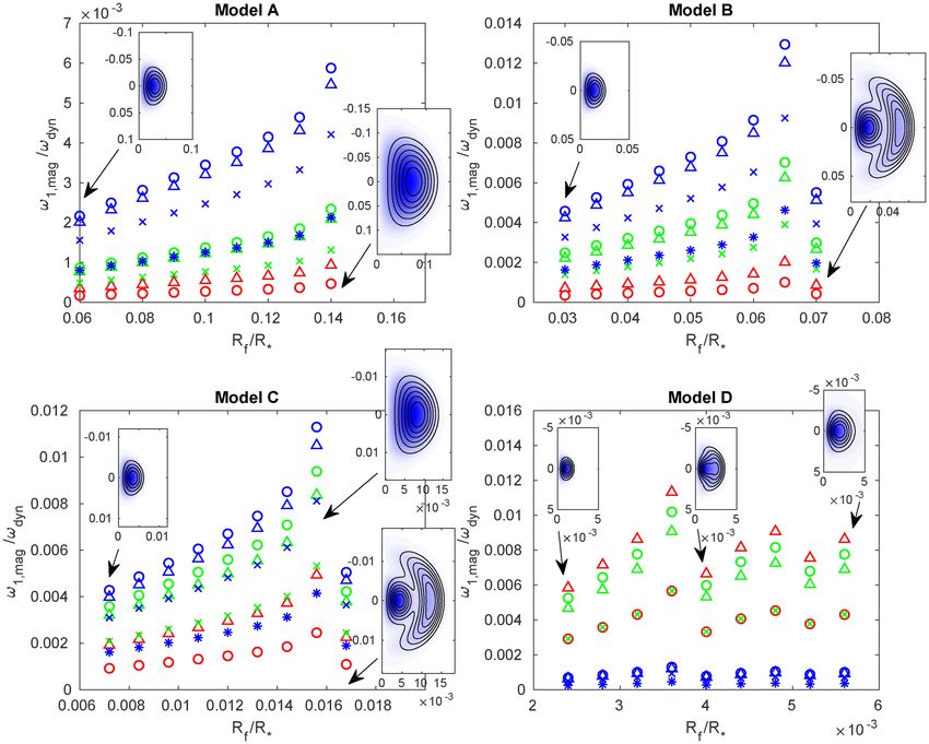
3712              S. T. Loi
Table 1. Summary of parameters for the four stellar        models, including their    expansion of their envelopes upon leaving the main sequence, and
mass M∗ , radius R∗ , dynamical frequency ωdyn = GM∗ /R∗3 , dynamical                  so rotational effects may be treated perturbatively. As mentioned
                √
speed vdyn = GM∗ /R∗ , grid size, range of oscillation frequencies ω                   above, the existence/properties of magnetic fields in red giant cores
considered, number of modes found, rotation frequency , radial extent                 is still largely speculative. While a sizeable fraction may have strong
of the magnetic field Rf , central Alfvén speed v A, cen , corresponding value of
                                                                                       fields that explain their mode depression, detailed predictions of how
the central field strength Bcen , and an estimate of the critical strength Bcrit for
comparison. Note that values of Rf and v A,cen shown are defaults. In some
                                                                                       weaker magnetism might impact the seismic properties of evolved
parts of this paper differing values are used, but where this occurs it will be        stars have been lacking. In particular, there are few studies examining
explicitly stated. Otherwise, the default values should be assumed.                    the simultaneous consequences of rotation and magnetism in these
                                                                                       objects, although several works have attempted to quantify the effects
Model                      A               B               C               D           of magnetism by itself (Cantiello, Fuller & Bildsten 2016; Gomes &
                                                                                       Lopes 2020; Loi 2020b). The recent works of Mathis et al. (2021)
Type                   Polytrope       Polytrope         MESA            MESA
                                                                                       and Bugnet et al. (2021), which have included the effects of aligned
                       (η = 4.2)       (η = 4.6)      (subgiant)      (red giant)
                                                                                       rotation in addition to a large-scale axisymmetric field, have begun

                                                                                                                                                                  Downloaded from https://academic.oup.com/mnras/article/504/3/3711/6225807 by guest on 18 September 2021
M∗ /M                    2.00            2.00           2.00            2.00
R∗ /R                    6.00            6.00           4.28            7.84
                                                                                       to fill these gaps. However, all the above works have assumed field
ωdyn /2π (μHz)            9.64            9.64           16.0            6.45          configurations that are simple and large scale. In contrast, the current
v dyn (m s−1 )         2.5 × 10⁵       2.5 × 10⁵      3.0 × 10⁵       2.2 × 10⁵        work aims to treat the unexplored regime of more complex radial
Number of grid           9565           101033         5 × 10⁴         5 × 10⁵         field structure that may also be misaligned with respect to rotation
points                                                                                 (i.e. non-axisymmetric).
ω/ωdyn                   0.5–1           0.5–1          8–12            8–12              It is the goal of this work to perform a phenomenological study
Number of modes        23 ( = 1)     72 ( = 1)      13 ( = 1)     71 ( = 1)        into the combined effects of rotation and magnetism on mixed modes
                       40 ( = 2)     124 ( = 2)     19 ( = 2)     121 ( = 2)       in evolved stars, where both Coriolis and Lorentz forces are assumed
                       56 ( = 3)     175 ( = 3)     26 ( = 3)     170 ( = 3)       to be weak enough that first-order perturbation theory applies. The
/ωdyn                   0.002           0.002           0.01           0.03
                                                                                       focus lies on low-degree mixed modes of short radial wavelength,
Rf /R∗                     0.1           0.05           0.012           0.004
v A, cen /v dyn          10−4          2 × 10⁻⁵       2 × 10⁻⁴        2 × 10⁻⁵
                                                                                       and the regime where the two forces are comparable in strength.
Bcen (MG)                 0.04           0.02              1             0.4           Axisymmetric ‘twisted torus’ configurations for the magnetic field
Bcrit (MG)                100             50              15              2            will be used, and allowed to be inclined with respect to the rotation
                                                                                       axis. This is motivated by the knowledge that rotation and magnetic
                                                                                       axes often do not coincide, as seen both in stars with fossil fields
   The mode depression phenomenon, which is exclusive to those                         (Henrichs et al. 2013; Braithwaite & Spruit 2017) and in objects
red giant stars >1.2 M (previously able to host core dynamos                          with active dynamos including the Sun (Gosling 2007) and the Earth
when on the main sequence), occurs in only a fraction of these                         (Merrill 2010). Rotation will be treated as uniform for simplicity;
(∼50 per cent for those >1.6 M ; Stello et al. 2016). It is therefore to              note that in the core region this would be physically justified as mag-
be wondered what explains the remaining stars: might they also have                    netic fields tend to enforce solid-body rotation (Spruit 1999). Besides
significant core fields but just below the critical threshold needed                   obliquity of the field, the impact of topology will also be examined,
for mode depression, or is there a genuine dichotomy in the field                      by considering twisted torus configurations of more complex radial
strengths/properties? Since magnetic fields are not spherically sym-                   structure. Note that no good knowledge exists about the most likely
metric, the Lorentz force lifts the degeneracy of modes with the same                  field topologies that may be found in red giant cores. Speculatively,
radial order n and spherical harmonic degree  but different azimuthal                 given that the most well-observed dynamos exhibit periodic reversals
order m, producing frequency splitting and giving rise to a multiplet.                 on relatively short time-scales (Jacobs 1994; Ossendrijver 2003), and
Similarly, the Coriolis force (arising from rotation) also produces                    simulations of stellar core dynamos show similar behaviour (Brun
frequency splitting (Beck et al. 2012; Mosser et al. 2015). At low ro-                 et al. 2005), one might imagine that as the convective core recedes
tation rates and/or weak fields, this problem can be treated using first-              over the main sequence it might leave behind magnetised shells of
order perturbation theory, which calculates the frequency correction                   alternating sign. Whether or how such small-scale complex structure
to the associated unperturbed eigenmode, assuming that the Coriolis                    (if it can survive to later stages) might influence frequency splittings
and Lorentz forces are small compared to pressure and buoyancy.                        has not previously been studied. It is to be noted that configurations
This approach has been used to treat solar p-modes (Gough &                            with larger spatial scales are lower in energy and expected to be
Thompson 1990), fundamental/low-order p-modes in Cepheid vari-                         more stable (Broderick & Narayan 2008; Duez & Mathis 2010).
ables (Shibahashi & Aerts 2000), and r-modes in degenerate stars                       However, we consider here the possibility that some dynamos may
(Morsink & Rezania 2002) under the influence of rotation and mag-                      preferentially create fields of smaller-scale structure, which may or
netism. For g-modes, the effects of a magnetic field were investigated                 may not eventually collapse to a lower energy state.
by Hasan, Zahn & Christensen-Dalsgaard (2005) for slowly pulsating                        This paper is structured as follows. In Section 2, we introduce the
B-stars, and Rashba et al. (2007) in the case of the Sun.                              stellar models and magnetic field configurations. In Section 3, we
   At larger rotation rates/field strengths, e.g. where the rota-                      describe how the basic (unperturbed) eigenmodes were computed,
tion/Alfvén frequency is a substantial fraction of the mode frequency,                and review relevant aspects of first-order perturbation theory. Results
non-perturbative approaches must be used. For example, there is a                      are presented in Section 4 and discussed further in Section 5, which
body of recent work on rapidly rotating stars where the Coriolis                       covers implications for asteroseismic inference and limitations of the
force is included via the traditional approximation (Buysschaert                       framework. Finally, we conclude in Section 6.
et al. 2018; Prat et al. 2019, 2020; Van Beeck et al. 2020), and
first-order perturbation theory is used for the Lorentz force only.
                                                                                       2 MODELS
This is relevant for massive main-sequence stars, for which magnetic
braking does not efficiently operate to slow down their rotation. In                   Four stellar models were examined in this study, all of mass
contrast, evolved stars rotate much more slowly due to the huge                        M∗ = 2 M . Two are polytropes of differing index, and two are

MNRAS 504, 3711–3729 (2021)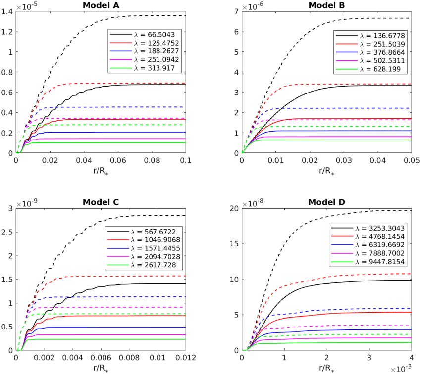
Magnetic field topology and obliquity                           3713

                                                                                                                                                                       Downloaded from https://academic.oup.com/mnras/article/504/3/3711/6225807 by guest on 18 September 2021
Figure 1. Background profiles showing the mass density ρ (left), gas pressure p (middle), and the Lamb and buoyancy frequencies S and N (right) for the two
polytropic models (A and B), of index η = 4.2 (top) and 4.6 (bottom). In the rightmost panels, S is plotted in red, green and blue for  = 1, 2, and 3, and N is
plotted in black. The dashed vertical lines indicate the default value of the field radius Rf used in most of the calculations. Note that S and N are shown plotted
up to the stellar surface, while the plots of ρ and p are zoomed in to the core region.

Figure 2. As in Fig. 1, but for the two MESA models (C and D). Note that plots of all quantities are zoomed in to the core region; the full stellar radii are 4.3
and 7.8R for Models C and D, respectively.

realistic evolved stellar models generated by the publicly avail-                    effects are too small to produce significant deformations away
able stellar evolutionary code ‘Modules for Experiments in Stel-                     from sphericity, or otherwise influence the hydrostatic background
lar Astrophysics’ (MESA, version r11701) (Paxton et al. 2011).                       structure. The magnetic field models were calculated separately
Their parameters are summarized in Table 1, and described in                         (see Section 2.3 for details), scaled to a desired strength and
further detail below. The structure of these models was computed                     imposed on the core region of each model within a boundary of
neglecting rotation and magnetism, as it is assumed that these                       radius Rf .

                                                                                                                             MNRAS 504, 3711–3729 (2021)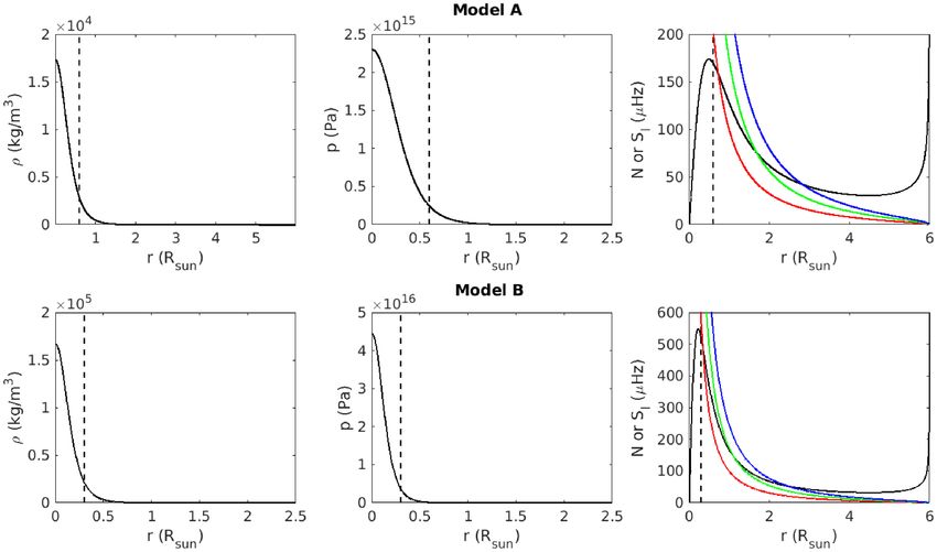
3714         S. T. Loi

                                                                                                                                                                    Downloaded from https://academic.oup.com/mnras/article/504/3/3711/6225807 by guest on 18 September 2021
Figure 3. Prendergast solutions for the first nine λ roots of Model C, shown in a meridional half-plane (note that the configurations are all axisymmetric). The
vertical axis coincides with the axis of symmetry of the field, while the horizontal axis plots the cylindrical radius. Contours show poloidal projections of the
field lines, while underlying colour indicates the strength of the toroidal component. Units on the colour bar are in MG. For the corresponding distributions of
the total field strength, and similar plots for the other stellar models, see Supplementary Figs S1–S7.

   The rotation profile is assumed to be uniform and described by                  2.1 Polytropes
a single scalar frequency , whose value is indicated in Table 1
                                                                                   Solutions to the Lane-Emden equation
for each of the models. For the polytropic models (A and B),
 was chosen to be a smallfixed fraction (0.2 per cent) of the                     1 d        2 dτ
                                                                                             χ        + τη = 0 ,                                             (1)
dynamical frequency ωdyn = GM∗ /R∗3 , where R∗ is the stellar                      χ 2 dχ        dχ
radius. For the MESA models (C and D),  was chosen to be consistent
                                                                                   which comes from substituting the polytropic relation p ∝ ρ 1 + 1/η
with characteristic rotational splittings of ∼100 nHz observed for
                                                                                   into the equations of hydrostatic equilibrium, provide simple models
dipole modes in red giant stars of around 2 M (Mosser et al.
                                                                                   for stars. Here, p is the gas pressure, ρ is the mass density, η is the
2012b, fig. 6). This translates to  values of about 1 per cent
                                                                                   polytropic index, χ is the radial coordinate, and τ is the polytropic
and 3 per cent of the dynamical frequencies of Models C and D,
                                                                                   temperature. These models are easy to generate and were considered
respectively.

MNRAS 504, 3711–3729 (2021)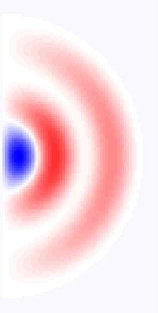
Magnetic field topology and obliquity                         3715

                                                                                                                                                                 Downloaded from https://academic.oup.com/mnras/article/504/3/3711/6225807 by guest on 18 September 2021
Figure 4. Frequencies ω0 (specified as a multiple of the dynamical frequency ωdyn ) and radial orders n of all modes with spherical harmonic degrees  = 1, 2,
and 3 obtained over the full search range. These are the modes in the spherically symmetric case (no rotation or magnetism).

in this study to see how much the results depended on the structure               Note that the values listed under ‘# grid points’ in Table 1 are only half
of the background.                                                                as large, as they refer to the size of the grid on which the eigenmodes
   Two polytropic models were generated, having the same mass                     were saved (this stems from the way the integration routine was
M∗ = 2 M and radius R∗ = 6 R , but different values of η. These                 implemented).
are referred to as Models A and B, where A has η = 4.2 and B has η =
4.6. The value of η controls the central condensation of a polytrope:
Model B has a smaller, denser core and larger, more tenuous envelope              2.3 Magnetic field
than Model A. These are shown in Fig. 1, which shows the radial                   Realistic modelling of magnetic fields in stars is a non-trivial task,
variation of p, ρ and the Lamb and buoyancy frequencies, S and N.                owing to the need to satisfy various physical and stability constraints.
A key difference between polytropes and realistic stellar models is               Besides the well-known solenoidal condition ∇ · B = 0, where B
that the former lack an evanescent zone between regions of p-mode                 is the magnetic field, all components of B need to be finite and
and g-mode propagation, and are non-convective throughout. Thus,                  continuous everywhere (to avoid infinite current sheets). If one
all modes in polytropes are heavily mixed, with substantial amounts               desires to model a spatially confined field (e.g. core of an evolved
of both p- and g-like character.                                                  star) then such a field cannot in general be force free (Spruit 2013).
                                                                                  Furthermore, any purely poloidal or purely toroidal configuration is
                                                                                  unstable and so only mixed configurations are allowed (Tayler 1973;
2.2 Evolved stellar models
                                                                                  Flowers & Ruderman 1977). Most simple configurations, including
A sequence of 2 M stellar models (with metallicity Z = 0.02) along               uniform vertical fields, purely toroidal fields, and dipole fields, which
a single evolutionary track was generated using MESA, the inlist of               have been widely used in many works, violate one or more of the
which is given in Appendix A. Two of the output models were se-                   above and are thus unlikely to be good descriptions of fields in reality.
lected for further analysis, corresponding to a subgiant (Model C) and            Instead, various analytical studies and numerical simulations point
a red giant (Model D), at ages of 976 Myr and 1.01 Gyr, respectively.             strongly towards so-called twisted-torus configurations (Prendergast
It was noticed that under the default settings of MESA a significant              1956; Braithwaite & Nordlund 2006; Yoshida, Yoshida & Eriguchi
level of jaggedness on the grid scale would be present. To remedy                 2006; Duez & Mathis 2010; Duez, Braithwaite & Mathis 2010b),
this, the mesh criteria were tightened to force MESA to use a finer               which are axisymmetric and dipole like in angular appearance (in the
grid, and further smoothing was applied to the outputs. The resultant             sense that they have two poles) but differ in several important ways
profiles of ρ, p, and N for Models C and D are shown in Fig. 2.                   from actual dipoles, namely that they have no central singularity,
   In more detail, the smoothing procedure involved first replacing               vanish smoothly at a finite radius, and possess a stabilizing toroidal
each point by that lying on the least-squares line of best fit through            component of comparable magnitude to the poloidal component.
the 13 neighbouring points (cf. boxcar smoothing), which were then                   Such configurations, despite being moderately complex in appear-
linearly interpolated to a uniform grid having the same number of                 ance, are surprisingly easy to construct analytically. This was first
points. This was downsampled by a factor of 5, and then spline                    achieved by Prendergast (1956) for incompressible fluids and later
interpolated to a uniform grid having a chosen final number of points,            generalized to the compressible case by Duez & Mathis (2010) and
which were 105 and 106 points for Models C and D, respectively.                   Duez et al. (2010b). The derivation will not be covered here; the

                                                                                                                        MNRAS 504, 3711–3729 (2021)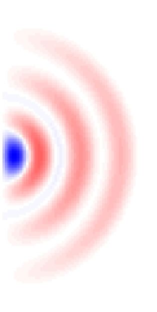
3716            S. T. Loi

                                                                                                                                                            Downloaded from https://academic.oup.com/mnras/article/504/3/3711/6225807 by guest on 18 September 2021
                                                                               Figure 6. Mode inertias calculated according to equation (10), for the two
                                                                               MESA models. These show minima corresponding to where the mode becomes
                                                                               more p-dominated. In the more evolved model (bottom), the pure g-mode
                                                                               spectrum is much denser than the pure p-mode spectrum, leading to fewer
Figure 5. Selected eigenfunctions computed in the non-rotating, non-           minima in the mixed-mode spectrum per given number of modes, compared
magnetic case (frequencies shown in Fig. 4). Black and red correspond to       to Model C (top).
the radial and horizontal components of the fluid displacement, R and H .
The associated model n and  are indicated in the panel headings. The mixed    to Rf , and in general there can be multiple roots due to the oscillatory
character of the modes is evident from the simultaneously substantial core
                                                                               nature of j1 . Roughly speaking, λ gives the inverse length scale of ,
and surface displacements in both cases. In the lower panel, which is for a
                                                                               and so larger λ roots correspond to configurations with progressively
more centrally condensed model, the inset shows a zoom-in to the core region
so that the g-mode oscillations can be better seen.                            finer radial structure. Once λ is chosen, is constructed as
                                                                                                                  r
                                                                                              λr
reader is encouraged to refer to the above works for details [also see            (r) ∝               fλ (r, Rf )      ρξ 3 j1 (λξ ) dξ
                                                                                          j1 (λRf )                 0
Loi (2020a) for a summary]. Although derived in the non-rotating                                     Rf
case, numerical work by Duez (2011) finds similar configurations in                       +j1 (λr)         ρξ 3 fλ (ξ, Rf ) dξ ,                     (5)
the presence of rotation, and these to be preferentially oblique with                              r
respect to the rotation axis. Such ‘twisted-torus’ field configurations        where fλ (r1 , r2 ) ≡ j1 (λr2 )y1 (λr1 ) − j1 (λr1 )y1 (λr2 ), and y1 is a
will be referred to here as Prendergast solutions.                             spherical Bessel function of the second kind. The final desired field
    Each Prendergast solution is completely described by two quan-             strength determines the scaling of .
tities: a scalar function of radius, (r), known as the radial flux                Prendergast solutions for the first nine λ roots of Model C are
function, and a parameter λ. These yield the magnetic field compo-             shown in Fig. 3. While the lowest order configuration may be
nents according to                                                             described as a twisted torus, higher order configurations take the
B = (Br , Bθ , Bφ )                                                     (2)    form of multiple nested tori. Note how the north–south projection
                                                                               of the field lines flips sign between radial shells, which one might
      2                                                                      imagine could mimic the end result of a periodically reversing
=      r2
            cos θ , − 1r   d
                           dr
                                sin θ , − λr sin θ       ,              (3)
                                                                               dynamo. Similar plots for the other stellar models, and corresponding
where (r, θ , φ ) are spherical polar coordinates defined with respect         distributions of the total field strength, are included as Supplementary
to the magnetic axis. Primes are used to distinguish the angular               Figs S1–S7. For the most part, the field strength is maximal at the
coordinates from those defined with respect to the rotation axis (i.e. θ       centre, with additional smaller local maxima at larger radii. Along
and φ), which is allowed to be different from the magnetic axis. The           the boundary r = Rf , all field components smoothly match to the
parameter λ must be a root of                                                  zero solution.
  Rf                                                                             The default values of Rf for each of the models are listed in Table 1,
      ρξ 3 j1 (λξ ) dξ = 0 ,                                         (4)       and marked in Figs 1 and 2. In the case of the MESA models, they
  0                                                                            were chosen to lie within the boundary of the former convective
where j1 is a spherical Bessel function of the first kind. Roots of            core, which was identified through inspection of the H and He
equation (4) will exist if ρ does not decrease too rapidly compared            composition profiles. The overall scaling of the field strength was

MNRAS 504, 3711–3729 (2021)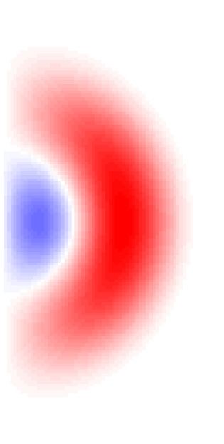
Magnetic field topology and obliquity                          3717

                                                                                                                                                                 Downloaded from https://academic.oup.com/mnras/article/504/3/3711/6225807 by guest on 18 September 2021
                                                                                 Figure 9. Top row: Structure of the matrices Mmag and Mrot , whose diagonal
                                                                                 entries directly give the value of the corotating-frame frequency shift in
                                                                                 units of ωdyn = GM∗ /R∗3 . Bottom row: The eigenvectors of (22), i.e. the
                                                                                 coefficients of expansion of corotating-frame modes with respect to the basis
                                                                                 of inertial-frame modes, in the case of alignment (left) and misalignment by
                                                                                 an angle of π /3 (right). These values were calculated for a p-dominated mode
                                                                                 of Model C with n = −16,  = 1. Rotation and field strength were set to their
                                                                                 default values listed in Table 1.

Figure 7. Inertial-frame frequency shifts versus unperturbed mode frequency
(expressed as a multiple of the dynamical frequency) for Model C, where the
different colours correspond to three cases: black dots are for zero field,
red plusses are for non-zero field (of the default strength listed in Table 1)
with β = 0, and blue crosses are for the same field strength but with
β = π /4. In all three cases the default rotation profile has been applied,
which is  = 0.01 ωdyn for this model. The 2 + 1 curves of the same
colour in each panel correspond to the different modes in the multiplet; for
the blue case, the component with the largest |am | has been selected for
plotting.

                                                                                         Figure 10. As for Fig. 9, but a mode with n = −28,  = 2.

                                                                                 controlled through the central Alfvén speed, the default values of
                                                                                 which are also listed in Table 1. These were chosen such that the
                                                                                 magnetic contribution to the frequency splitting would be about the
                                                                                 same order as that due to rotation. For comparison, the critical field
                                                                                 strength (Fuller et al. 2015; Loi 2020a) is also listed in the table,
                                                                                 which marks the transition to dynamically significant field strengths
                                                                                 where perturbation theory would be invalid.

                                                                                 3 METHODS

                                                                                 3.1 Basic eigenmodes

             Figure 8. As for Fig. 7, but Model D and  = 1.                     First, we need to obtain the set of basic eigenmodes that exist in
                                                                                 the absence of rotation and magnetism. The time-dependent fluid
                                                                                 displacement vector field for a normal mode of frequency ω can be

                                                                                                                        MNRAS 504, 3711–3729 (2021)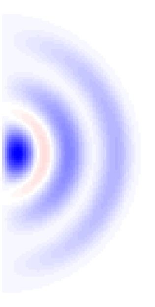
3718          S. T. Loi
                                                                            radial orders and frequencies that scale roughly as 1/|n|. Examples
                                                                            of the associated eigenfunctions are shown in Fig. 5, where the finest
                                                                            scales of variation can be seen to occur in the deep interior. A useful
                                                                            measure of the p- or g-like character of a mode is the mode inertia:
                                                                                   R∗ 2  2
                                                                                    0 ρr    R (r) + ( + 1)H2 (r) dr
                                                                            I =                                          ,                    (10)
                                                                                       R2 (R∗ ) + ( + 1)H2 (R∗ )
                                                                            which measures the mass of fluid displaced and is larger for modes
                                                                            localized to the core where ρ is larger, i.e. g-dominated modes. Fig. 6
                                                                            shows the values of I for all modes of Models C and D. The small
                                                                            number of modes with very low inertia correspond to the p-dominated
                                                                            modes, which occur near the frequencies of pure envelope p-modes.
                                                                            For Models A and B, their lack of an evanescent zone means that I

                                                                                                                                                      Downloaded from https://academic.oup.com/mnras/article/504/3/3711/6225807 by guest on 18 September 2021
                                                                            values are relatively constant over the considered frequency range;
                                                                            these are not shown.

                                                                            3.2 First-order perturbation theory
          Figure 11. As for Fig. 9, but a mode with n = −49,  = 3.
                                                                            To calculate frequency corrections to the basic eigenmodes induced
                                                                            by rotation and magnetism, first-order perturbation theory was used,
written
                                                                            which is a standard formalism (e.g. see Dziembowski & Goode 1984;
ξ (r, θ, φ, t) = ξr (r, θ, φ)r̂ + ξθ (r, θ, φ)θ̂ + ξφ (r, θ, φ)φ̂           Unno et al. 1989). It is valid in the limit of small perturbing forces,
                                                                            which is the regime focused on here. This section overviews relevant
                  exp(−iωt) ,                                         (6)
                                                                            aspects of this theory, in particular its application to the problem of
where                                                                       misaligned rotation and magnetism.
                                                                               The presence of a non-spherically symmetric force (e.g. Coriolis
ξr (r, θ, φ) =         R,m (r)Ym (θ, φ) ,                                 and Lorentz) lifts the degeneracy otherwise possessed by modes of
                 ,m
                                                                            the same n and  but different m. For a given , there exist 2 + 1
                                  ∂ m                                       values of m going from − to +. To first order, pure rotation of
ξθ (r, θ, φ) =         H,m (r)     Y (θ, φ) ,
                 ,m
                                  ∂θ                                       frequency  perturbs the mode frequencies by a value proportional
                       H,m (r) ∂ m                                         to m, giving a multiplet of 2 + 1 peaks. On the other hand, pure
ξφ (r, θ, φ) =                   Y (θ, φ) .                           (7)   magnetism of characteristic field strength B perturbs the frequencies
                        sin θ ∂φ
                 ,m                                                        by a value proportional to B2 and independent of the sign of m,
Note that torsional motions have been neglected as the only restoring       giving a multiplet of  + 1 peaks where modes of the same |m|
forces at this stage are pressure and buoyancy. Also, for spherically       continue to experience a degeneracy. Note that this statement applies
symmetric backgrounds R, m and H, m will not depend on m, so we           to axisymmetric fields, for which the quantum numbers  and m can
shall write R, m → R , H, m → H .                                       be defined, and not for general non-axisymmetric fields where  and
   Substituting into the equations of motion and linearizing, and           m would lose their meaning.
projecting out a single spherical harmonic, we get the equations of            Under the combined influence of the two effects, the picture
stellar oscillation                                                         is more complicated. From the point of view of the star (i.e. in
                                                                          the stationary/corotating frame), there can still be only 2 + 1
 dR
       = (+1)
              r
                  − γρrp ω2 H − 2r + γ1p dpdr
                                                 R ,              (8)      frequencies since that is the number of originally degenerate modes.
  dr
                                                                           Under axisymmetric conditions (aligned rotation and magnetic axes)
 dH                2               −1 1
       = 1r 1 − Nω2 R − ρN 2 dp            + r H .               (9)      each of these is associated with a different m, and from the point of
                                      dr
  dr                                                                        view of an observer (i.e. in the inertial frame) there are thus 2 +
Note that we have made the Cowling approximation (suitable for              1 peaks, where the frequencies are additionally Doppler shifted by
modes with small radial scales) thus reducing the system to second          a value of m. This is similar to the pure rotation case, except that
order, and neglected spatial variations of the adiabatic index γ .          due to the Lorentz force the multiplet may exhibit asymmetries; for a
   The eigenmodes used for subsequent analysis in this work were            complete discussion and seismic diagnosis of these asymmetries,
obtained by directly solving equations (8) and (9) under appropriate        we refer the reader to the detailed discussion in Bugnet et al.
boundary conditions (regularity at r = 0, and vanishing Lagrangian          (2021). Under non-axisymmetric conditions (misaligned rotation
pressure perturbation at the surface). They were solved via standard        and magnetic axes), there would still be 2 + 1 modes in the
methods (shooting with a fourth-order Runge–Kutta scheme and                stationary/corotating frame, but now each mode can no longer be
matching at an intermediate radius) to obtain a set of unperturbed          associated with a single m since the system has no axis of symmetry.
eigenmodes for spherical harmonic degrees  = 1, 2, and 3 over              Rather, each would be an admixture of the 2 + 1 different values of
chosen ω ranges. These were [0.5, 1] ωdyn for Models A and B, and           m, giving rise to (2 + 1)2 peaks in the inertial frame after Doppler
[8, 12] ωdyn for Models C and D. The numbers of modes found within          shifting. Their amplitudes are directly related to the coefficients of
each interval are listed in Table 1. The radial order n of the various      expansion: for example, in the limit of mutual alignment (which is a
modes was computed using the Eckart (1960) scheme.                          special case of this more general framework), a single m dominates
   Fig. 4 plots the frequencies and radial orders of all modes. The         strongly for each corotating-frame mode and thus only 2 + 1 out of
vast majority of these are highly g-dominated, with large negative          (2 + 1)2 possible peaks have non-zero amplitudes.

MNRAS 504, 3711–3729 (2021)
Magnetic field topology and obliquity 3719
Downloaded from https://academic.oup.com/mnras/article/504/3/3711/6225807 by guest on 18 September 2021
Figure 12. Splitting diagram for a p-dominated mode of Model C, with n = −16 and = 1 (i.e. that used in Fig. 9), under the default rotation and field strength
listed in Table 1, for six different values of the obliquity angle. Short, thick, horizontal black lines joined by thin dotted lines illustrate the splitting process,
from the unperturbed mode (leftmost line at ω1 = 0) into a multiplet of 2 + 1 modes in the corotating frame (middle group), and then further into (2 +
1)2 modes in the inertial frame (rightmost group). In the rightmost group, the various modes have been horizontally offset for clarity. The different grey-scale
shades correspond to the absolute value of the associated am coefficient, with black being 1 (maximum amplitude) and white being 0. For comparison, horizontal
coloured dashed lines mark the position of the non-magnetic rotationally split multiplet in the inertial frame.
Figure 13. As for Fig. 12, but a mode with n = −28 and = 2 (i.e. that used in Fig. 10).
The mathematical treatment is as follows. Let m and m be defined that m < 0 modes are prograde). The equation of motion can be
as the azimuthal quantum numbers with respect to the rotation and written
magnetic axes, respectively, and let β be the obliquity angle. Let
ω and ω̄ be the frequencies in the inertial and corotating frames,
respectively, and thus related by ω̄ = ω + m (this definition means ω̄2 ξ = L0 ξ + Lrot ξ + Lmag ξ , (11)
MNRAS 504, 3711–3729 (2021)3720 S. T. Loi
where Lrot and Lmag , which correspond to the Coriolis and Lorentz where the summation is such that the factorials are non-negative.
forces, are assumed to be much smaller than L0 , which represents These satisfy
the combination of pressure and buoyancy. Their functional forms in
terms of the fluid displacement ξ and background quantities are Ym (θ, φ) = + () m
m =− dmm (β) Y (θ , φ ) , (20)
∇p which when substituted into (7) leads to
L0 ξ = (ρ∇ · ξ + ξ · ∇ρ) − ρ1 ∇ (γ p∇ · ξ + ξ · ∇p) , (12)
ρ2
ξ 0,m (r, θ, φ, t) = + ()
m =− dmm (β) ξ 0,m (r, θ , φ , t) . (21)
Lrot ξ = 2iω̄ × ξ + × ( × ξ ) , (13)
Hence, equation (18) can be expressed as a = Da , where a = (am :
1 m = −, · · · , +) and a = (am : m = −, · · · , +). We can then
Lmag ξ = B × {∇ × [(B · ∇)ξ − B(∇ · ξ ) − (ξ · ∇)B]}
ρ recast equation (17) in the more general form of a matrix eigenvalue
1 problem:
+ [∇ × (ξ × B)] × (∇ × B)
ρ ω̄1 a = Mrot a + DMmag D a , (22)
Downloaded from https://academic.oup.com/mnras/article/504/3/3711/6225807 by guest on 18 September 2021
1
− 2 (ρ∇ · ξ + ξ · ∇ρ) (∇ × B) × B. (14) where the Wigner d-matrix has the property that D−1 = D , and
ρ
diag( Lrot ξ 0,m , ξ 0,m : m=−,··· ,+)
The goal is to solve for the first-order frequency corrections ω̄1 , Mrot = 2ω0 ξ 0 , ξ 0
, (23)
where ω̄ = ω0 + ω̄1 + · · · . Here, ω0 is the frequency associated with
the unperturbed eigenmode ξ 0 , where ξ = ξ 0 + ξ 1 + · · · . Substitut- diag Lmag ξ 0,m , ξ 0,m : m =−,··· ,+
Mmag = 2ω0 ξ 0 , ξ 0
. (24)
ing these expansions into equation (11) and truncating at first order
gives It is easy to see that this reduces to the aligned case when β =
L1 ξ 0 + L0 ξ 1 = ω02 ξ 1 + 2ω0 ω̄1 ξ 0 , (15) 0 ⇒ D = I, in which case the eigenvectors a are simply the columns
of I. The vectorial nature of a is not to be confused with a spatial
where L1 = Lrot + Lmag . Now L0 is self-adjoint, implying that {ξ 0 } coordinate vector; rather, it is a coordinate representation of the
form a complete
orthogonal basis. Therefore, it is possible to express admixture of m, with 2 + 1 components.
any ξ 1 = k ck ξ 0(k) , where k is some enumeration of the set of {ξ 0 }. A word of caution is to be made about the self-adjointness of
Combining this with the fact that ω02 ξ 0 = L0 ξ 0 , the Lorentz operator Lmag . In the fully self-consistent case where
deformation is taken into account, the combined operator in equation
(j )
L1 ξ 0 +
(j )
ck ω0 − ω0 (k)2 (j )2 (k) (j ) (j ) (j )
ξ 0 = 2ω0 ω̄1 ξ 0 (16) (11) would be self-adjoint thus producing real frequencies, which
k
is expected in ideal MHD. Note that in practice this deformation
is small, and its dynamical consequences can largely be neglected
for some eigenmode labelled j (with chosen n and ). (Duez, Mathis & Turck-Chièze 2010a). As it stands, L0 and Lrot
(j )
If L1 were axisymmetric, it would suffice to consider ξ 0 as being defined in equations (12) and (13) are self-adjoint, but Lmag as defined
made up of a single m. Then, we would be able to take the inner in equation (14) is not. The approximations used thus have the side
(j )
product of equation (16) with ξ 0,m , which is defined to be (6) but effect of introducing imaginary components to the frequencies that
restricted to a fixed m, and use orthogonality to get are not physical. However, there exists a convenient remedy in the
(j ) (j ) form of retaining only the first term on the RHS of equation (14),
1 L1 ξ 0,m , ξ 0,m
(j )
ω̄1,m = . (17) which is the dominant term for modes of short wavelength and also
(j ) (j ) (j )
2ω0 ξ0 , ξ0 happens to be self-adjoint. Hence, we make the approximation
1
The inner product is defined as ξ , η = ρξ ∗ · η dV , where the Lmag ξ ≈ B × {∇ × [(B · ∇)ξ − B(∇ · ξ ) − (ξ · ∇)B]} . (25)
ρ
integral is over the volume of the star. However, if β = 0 then L1
will not be axisymmetric, even if Lrot and Lmag individually are. In Also, since rotation frequencies are assumed to be small, we neglect
this case, L1 mixes the different m, and equation (17) needs to be the second (centrifugal) term in Lrot in favour of the first (Coriolis):
replaced by a (2 + 1) × (2 + 1) matrix equation. Let us write
Lrot ξ ≈ 2iω0 × ξ . (26)
+ +
ξ 0 (r, θ, φ, t) = am ξ 0,m = ξ 0 (r, θ , φ , t) = am ξ 0,m , The L0 term is left as is. With these simplifications, the elements of
m=− m =− Mrot and Mmag are then
(18)
Lrot ξ 0,m , ξ 0,m = 4ω0 ρ Im ξφ ξθ∗ cos θ + ξr∗ sin θ dV ,
where ξ 0,m has the same form as ξ 0,m but with (m, θ, φ) → (m , θ , (27)
φ ), and we have dropped the labels j with the understanding that all
quantities now pertain to the mode j.
Lmag ξ 0,m , ξ 0,m = Bθ Jφ∗ − Bφ Jθ∗ ξr
To transform between coordinate frames (r, θ , φ) and (r, θ , φ ),
we invoke the Wigner d-matrix, denoted here by D. Its entries are + Bφ Jr ∗ − Br Jφ∗ ξθ
given by
+ Br Jθ∗ − Bθ Jr ∗ ξφ dV , (28)
() 1/2
dmm (β) = ( + m)!( − m)!( + m )!( − m )!
⎡ where ξ r , ξ θ , ξ φ in equation (27) refer to the components of ξ 0,m , and
2+m −m−2s β m−m +2s ⎤
(−1)m−m +s cos β2 sin 2 ξr , ξθ , ξφ in equation (28) refer to the components of ξ 0,m . Here,
× ⎣ ⎦, J = (Jr , Jθ , Jφ ) is the Eulerian perturbation to the current density.
s
( + m − s)!s!(m − m + s)!( − m − s)!
Expressions for the components of J for the special case of the
(19) Prendergast solution can be found in Appendix B.
MNRAS 504, 3711–3729 (2021)Magnetic field topology and obliquity 3721
Downloaded from https://academic.oup.com/mnras/article/504/3/3711/6225807 by guest on 18 September 2021
Figure 14. As for Fig. 12, but with a field strength three times higher.
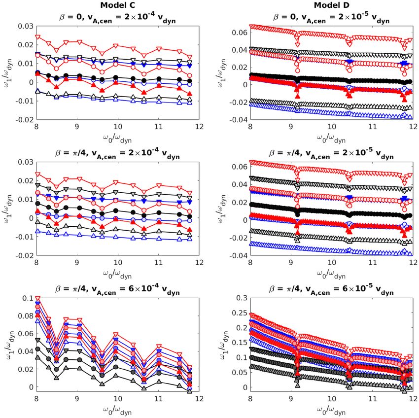
4 R E S U LT S have been chosen for plotting in Figs 7 and 8; these correspond to
the m components with the largest |am | values, i.e. largest observed
4.1 Comparison with pure rotation amplitudes. As the field strength and/or obliquity increase, it becomes
less easy to identify the m component with the largest |am |, as the
Figs 7 and 8 show the inertial-frame frequency shifts ω1 = ω̄1 − m
various |am | values become comparable.
for Models C and D as a function of ω0 , for three different cases: pure
The m-mixing process is illustrated in Figs 9–11, for a chosen
rotation (black), rotation plus magnetic field where β = 0 (red), and
mode of Model C with = 1, 2, and 3. The values of , v A, cen
rotation plus magnetic field where β = π/4 (blue). Comparing the red
and Rf are the same in all cases. Along the top row of each plot are
curve with the black curve, two aspects can be noted: (i) p-dominated
the matrices Mmag and Mrot , whose entries quantitatively represent
multiplets are more symmetric than g-dominated ones and (ii) the
the corotating-frame frequency shift that would be induced by each
asymmetries are more pronounced at lower frequencies. The first
effect in the absence of the other. Along the bottom row are matrices
point can be explained by the fact that the magnetic field is confined to
containing the 2 + 1 eigenvectors of equation (22), where each
the core where g-dominated mixed modes are localized; p-dominated
column corresponds to one eigenvector. These are shown for two
mixed modes are thus more similar to modes in the case of pure
values of β. When β = 0 (aligned case) these yield the identity
rotation, for which ω1 is roughly constant with ω0 . The second point
matrix (no m-mixing), but for β = π /3 (oblique case) the off-diagonal
can be understood through the frequency dependence of the elements
components are non-zero. Comparing the three values of , it can be
of Mrot and Mmag . While Mmag ∝ 1/ω0 , the factors of ω0 in Mrot
seen that the magnetic contribution to the frequency shifts, given
cancel out in the numerator and denominator, leaving no explicit ω0
by the components of Mmag , increases for higher . Physically this
dependence. The increased importance of magnetic effects at lower
can be understood from the fact that for modes possessing g-like
frequencies can be physically understood in terms of the increase
character, larger are associated with smaller spatial scales and
of the Alfvén frequency ωA ∝ k, where k is the wavenumber, thus
therefore larger Alfvén frequencies, for the same ω0 . In contrast, the
bringing it closer to the mode frequency. Note that we are in the
rotational contribution, given by the components of Mrot , decreases
regime where ωA ω0 and that ωA ∼ ω0 corresponds to the strong-
for increasing given the same m. Consequently, the amount of
field (dynamically significant) regime in which perturbation theory
m-mixing increases with for the same obliquity.
breaks down.
Figs 12–14 illustrate the splitting process for a chosen mode of
It is curious to note that for = 1, in both Models C and D, the
Model C for six different values of β going from 0 (aligned) to π /2
blue curves (β = π /4) exhibit more symmetric splittings than the red
(perpendicular). Similar plots for Models A and D can be found in
(β = 0). This appears to roughly hold across the whole frequency
Supplementary Figs S8–S13. It can be seen that greater m-mixing
range. However, the = 2 case does not show this behaviour, at least
occurs for intermediate obliquities (β ∼ π /4), higher , and larger
for the value of β tested.
field strengths. In Fig. 12, it is apparent that in the inertial frame
only 2 + 1 out of (2 + 1)2 peaks dominate, consistent with
the a matrix remaining approximately diagonal even at substantial
4.2 Effect of obliquity obliquities (see Fig. 9). Closer inspection of how the shape of this
As mentioned in Section 3.2, an important consequence of obliquity dominant sub-multiplet changes with obliquity reveals that while this
is to mix the different m components, giving rise to (2 + 1)2 may be asymmetric in general, it is still possible for this to appear
frequencies in the inertial frame. However, only 2 + 1 blue curves nearly symmetric for some values of β and have a spacing close to
MNRAS 504, 3711–3729 (2021)3722 S. T. Loi
Downloaded from https://academic.oup.com/mnras/article/504/3/3711/6225807 by guest on 18 September 2021
Figure 15. Inertial-frame frequency shifts versus unperturbed frequency, for all = 1 modes of Models C (left) and D (right). Values of the field strength and
obliquity are shown in the panel headers. Within each panel, the different colours correspond to the corotating-frame modes, which are each split further into
2 + 1 modes in the inertial frame. The different symbols represent the different m components: upward triangles represent m = +1 (retrograde modes), circles
represent m = 0, and downward triangles represent m = −1 (prograde modes). In addition, each symbol is filled with a colour whose saturation varies according
to the value |am |. Fully saturated (i.e. solid red/blue/black) corresponds to |am | = 1, while white corresponds to |am | = 0.
the value expected of pure rotation (Fig. 12, lower left-hand panel). default values of Rf for each model used in preceding sections are
However, the centroid of this sub-multiplet is offset compared to indicated in Table 1, but in this particular section we choose to vary
the pure rotational multiplet. At larger field strengths (see Fig. 14), Rf between 0.6 and 1.4 times the default, while keeping all other
there may be many peaks of significant amplitude in the inertial parameters (including v A, cen ) the same.
frame. Notably, due to the heavy mixing, it would be possible to Fig. 16 shows that the components of Mmag , representing the
find symmetric sub-multiplets among these (e.g. bottom row, middle magnetic contribution to the overall frequency shift, increase in rough
panel). proportion with Rf . This may be explained by the integral in equation
Frequency splittings for all = 1 modes of Models C and D (14) being larger when there is more volume of field to integrate over.
are summarized in Fig. 15, where points are coloured according to However, this trend is not strict, and in some cases as for Model D the
the associated value of |am |. The increased m-mixing with larger behaviour can be somewhat unpredictable. This appears to be tied
obliquity and field strength can clearly be seen across all modes, to the complicating influence of variations in geometry/topology of
both p- and g-dominated. The main difference between p- and g- the field as Rf is modified; this occurs for the Prendergast model
dominated mixed modes appears to lie in the centroid frequency of because of the dependence of (4) and (5) on ρ, whose shape over
the multiplet: this is located towards systematically higher values the interval r ∈ [0, Rf ] does not scale straightforwardly with Rf . At
compared to the unperturbed value for g-dominated multiplets, a points where the configuration acquires additional radial structure
feature not present in the case of pure rotation (as seen in Figs 7 and 8), (see inset panels), this tends to disrupt the trend. Further discussion
where the centroid offset is zero for all multiplets. This offset between of the field topology can be found in the next section.
p- and g-dominated multiplets increases towards lower frequencies, This plot also sheds light on the effect of central condensation.
where magnetic effects become more significant. Consider Models A and B, which are both polytropic models with
the same M∗ and R∗ (and therefore dynamical frequency), but have
different central condensations due to their differing polytropic
4.3 Radial extent of the field
indices. They also have similar central field strengths (differing by
When constructing each Prendergast field solution, one has free a factor of 2, being larger in Model A). However, the magnetic
choice over the parameter Rf , the radial extent of the field. The shifts in Model B are larger than A by a factor of about 2, and
MNRAS 504, 3711–3729 (2021)Magnetic field topology and obliquity 3723
Downloaded from https://academic.oup.com/mnras/article/504/3/3711/6225807 by guest on 18 September 2021
Figure 16. Magnetic contribution to the corotating-frame frequency shift (i.e. the components of Mmag ) as a function of the radial extent Rf of the field region,
for selected modes of each model. Red, green, and blue correspond to = 1, 2, and 3, respectively, while circles, triangles, crosses, and asterisks correspond
to |m | = 0, 1, 2, and 3, respectively. Inset plots show the field configurations for select values of Rf indicated by the arrows. Each set of like-coloured points
within each panel was generated for a single value of n. In order of increasing , these were n = −31, −50, −75 for Model A, n = −100, −179, −240 for
Model B, n = −16, −28, −49 for Model C and n = −151, −255, −397 for Model D. In the case of the two MESA models these choices of n correspond to
p-dominated modes (minima of Fig. 6).
since this scales with B2 , if Model B had the same central field Rf . The g-dominated modes are seen to be much more sensitive to
strength then the frequency shift would be ∼8 times larger than increases in Rf compared to p-dominated modes, as can be seen by
in Model A. The increased importance of magnetic effects at higher their larger values of ω1 . This can be attributed to their preferential
central condensations can be attributed to the smaller spatial scales of localization to the core, where the field is located.
oscillation in the core due to the larger buoyancy frequency, leading to
a higher Alfvén frequency. This effect is more difficult to disentangle
using Models C and D because the various modes differ wildly in their 4.4 Role of field topology
level of p-like versus g-like character, which represents a conflating As mentioned in Section 2.3, multiple values of λ can satisfy
influence. (4) for a given combination of Rf and ρ(r). These correspond to
A minor further comment about Fig. 16 concerns the -dependence fields of different topologies (cf. Fig. 3). Fig. 18 shows how the
for the different models. In Models A, B, and C, for which the modes components of Mmag vary as a function of λ. The general trend
chosen for plotting all have relatively large amounts of mixed p- and is for these to decrease with increasing λ, suggesting that fields
g-like character, higher undergo larger shifts since the dominant with more radial structure may produce smaller magnetic shifts,
factor is the shrinkage of spatial scales as increases (driving up the even if the central field strength is held constant. For Model D, the
Alfvén frequency). However, in Model D, which is more evolved trend is not so smooth (second and fourth λ values are outliers);
than Model C, the much greater p-dominated character for higher inspection of Supplementary Figs S3 and S7 shows that these have
means that the behaviour is reversed: higher values undergo smaller unusual field structure, possessing a node/minimum very near the
magnetic shifts. centre. The approach used here to control the field amplitude via
The inertial-frame frequency shifts (including the Coriolis force) scaling the central value thus produces anomalously large maximum
for all modes of Model C are shown in Fig. 17 for two values of field strengths and therefore frequency shifts. However, in all
MNRAS 504, 3711–3729 (2021)3724 S. T. Loi
might be expected, similar to the case for Rf , the g-dominated mixed
modes are far more sensitive to changes in λ than the p-dominated
ones.
5 DISCUSSION
5.1 Implications for asteroseismology
Multiplet asymmetries are a known consequence of the Lorentz
force, contrasting the Coriolis force which by itself only produces
symmetric multiplets in the limit of slow rotation. While it may
be tempting to use this signature as an indicator for the presence
or absence of core magnetism, there are several complications.
Downloaded from https://academic.oup.com/mnras/article/504/3/3711/6225807 by guest on 18 September 2021
First, magnetism is not the only possible cause of asymmetry
(cf. Deheuvels, Ouazzani & Basu 2017). Secondly, the results
here show that it is possible for multiplets to appear symmetri-
cally split, by a value close to that associated with pure rota-
tion, even when the Lorentz force is comparable to the Coriolis
force. This tends to occur for intermediate obliquities (β ∼ π /4);
see e.g. Figs 12 and 15 (middle row). This result is impor-
tant because it means that the detection of symmetric multiplets
cannot alone be used to rule out the existence of a magnetic
field.
A closely related concern is the fact that magnetic fields of non-
zero obliquity are supposed to increase the multiplicity from 2
Figure 17. Inertial-frame frequency shifts versus unperturbed frequency for + 1 to (2 + 1)2 peaks in the inertial frame. Given this, it might
all modes of Model C, for two different values of Rf , these being 0.7 (top) be similarly tempting to interpret the observed lack of additional
and 1.3 (bottom) times the default value listed in Table 1. Rotation and multiplicity as evidence of the absence of a magnetic field. However,
field strength are set to their default values, and β = 0. Red, green, and it is clear from e.g. Fig. 9 (bottom right) that most of the additional
blue correspond to = 1, 2, and 3, respectively, while different symbols components can have quite low amplitudes, perhaps an order of
correspond to different values of m . In increasing order from m = −3 to magnitude smaller than the dominant components, even in situations
+3, these are denoted by pentagrams, squares, downward triangles, circles, where the Lorentz force is comparable to the Coriolis force and β
upward triangles, diamonds, and asterisks, respectively.
is substantial. Thus in practice, many of the additional peaks may
not stand out well above the noise, and only the 2 + 1 dominant
components along the diagonal of the a matrix have sufficient
other cases the central and maximum field strengths are virtually amplitudes to be identified. It is therefore possible that magnetic
identical. fields of substantial strengths are present in stars for which this
Further insight into the cause of this systematic behaviour with scenario has previously been ruled out on the basis of the lack
λ comes from inspecting the spatial contribution of the integrand of multiplet asymmetry and/or absence of enhanced multiplicity.
defined in equation (14), by considering the value of the integral Rather, more detailed modelling on a case-by-case basis may be
evaluated from 0 to some finite r rather than all the way up to the required to support such conclusions.
stellar surface. Fig. 19 plots this as a function of the integration There may be some specific behaviours that could provide
limit r, for the = 1 modes used in Fig. 18. While some small- useful arguments for or against the existence of a core magnetic
scale fluctuations resulting from the mode structure are present, the field. As noted throughout Section 4, magnetic effects are more
overall behaviour in all cases is a relatively steep increase in the most important for modes with shorter wavelengths and higher inertias.
central regions, where the rate of growth is largely independent of λ. Signatures such as multiplet asymmetry and enhanced multiplicity
Further out where the configurations undergo their finer-scale spatial are therefore expected to be most pronounced for modes that
reversals, the integrals plateau to a constant value that is lower for have lower ω0 , higher , are more g-dominated, and in stars with
larger λ. Since all curves are monotonically increasing (if one ignores greater central condensations. In particular, the 1/ω0 dependence of
the small-scale fluctuations), this means that the integrand is always the magnetic shift and its tendency to systematically increase the
positive and so we conclude that for larger λ, it must be that the centroid frequency of a multiplet is in contrast to the behaviour
integrand itself is smaller over more of the volume. With aid of of rotation, which at leading order has no ω0 dependence and
the plots showing total field strength (Figs S4–S7), it is apparent does not alter the centroid frequency. Since g-dominated mixed
that this is driven by the steeper drop-off in field strength with radial modes are more heavily affected by a core field, the centroids
distance for configurations with larger λ. Whether this is a peculiarity of their associated multiplets would be displaced further from the
of the Prendergast solution or likely to be a property of real stellar unperturbed values compared to p-dominated mixed modes. For
magnetic fields is unknown. However, it is to be noted that a separate example, if one were to perform forward modelling of an evolved
physical argument for weaker overall field strength in regions star to reproduce well the p-dominated mode frequencies while
possessing smaller scale field structure is the higher rate of Ohmic neglecting the existence of a core field, then this would systematically
dissipation. underpredict the frequencies of g-dominated modes. The discrepancy
The inertial-frame frequency shifts (including the Coriolis force) would be worse at lower ω0 and higher . Demonstration of
for all modes of Model C are shown in Fig. 20, for two values of λ. As such behaviour or lack thereof could provide a convincing case
MNRAS 504, 3711–3729 (2021)You can also read