The Polar Cap (PC) index combination, PCC: relations to solar wind properties and global magnetic disturbances
←
→
Page content transcription
If your browser does not render page correctly, please read the page content below
J. Space Weather Space Clim. 2021, 11, 19
Ó P. Stauning, Published by EDP Sciences 2021
https://doi.org/10.1051/swsc/2020074
                                                                                                                                     Available online at:
                                                                                                                                    www.swsc-journal.org

 RESEARCH ARTICLE                                                                                                                OPEN          ACCESS

The Polar Cap (PC) index combination, PCC: relations to solar
wind properties and global magnetic disturbances
Peter Stauning*
Danish Meteorological Institute, Lyngbyvej 100, DK-2100 Copenhagen, Denmark

              Received 24 April 2020 / Accepted 4 December 2020

              Abstract – The non-negative Polar Cap PCC index built from PCN (North) and PCS (South) indices
              correlates better with the solar wind merging electric field and is more representative for the total energy
              input from the solar wind to the magnetosphere and for the development of geomagnetic disturbances
              represented by the Kp index and ring current indices than either of the hemispheric indices. The present
              work shows that the ring current index, Dst, to a high degree of accuracy can be derived from a source
              function built from PCC indices. The integration of the PCC-based source function throughout the interval
              from 1992 to 2018 without attachment to the real Dst indices based on low latitude magnetic observations
              has generated equivalent Dst values that correlate very well (R = 0.86) with the real Dst index values,
              which are represented with a mean deviation less than 1 nT and an overall RMS deviation less than
              13 nT. The precise correlation between the real and equivalent Dst values has been used to correct the
              PCC indices for saturation effects at high intensity disturbance conditions where the Dst index may take
              values beyond 100 nT. The relations between PCC and the ring current indices, Dst and ASY-H have
              been used, in addition, to derive the precise timing between polar cap convection processes reflected in
              the polar cap indices and the formation of the partial and total ring current systems. Building the ring
              current is considered to represent the energy input from the solar wind, which also powers auroral distur-
              bance processes such as substorms and upper atmosphere heating. With current available PC indices,
              detailed and accurate SYM-H or Dst index values could be derived up to nearly one hour ahead of actual
              time by integration of the PCC-based source function from any previous quiet state. Thus, the PCC indices
              enabling accurate estimates of the energy input from the solar wind are powerful tools for space weather
              monitoring and for solar-terrestrial research.

1 Introduction                                                                    plasma flow (DP3) possibly inside a residual two-cell forward
                                                                                  convection system. Although many details have been added
    In the early Space Age, Dungey (1961) formulated the                          later, these solar wind-magnetosphere interaction models still
concept of magnetic merging processes taking place at the front                   prevail now, 60 years later.
of the magnetosphere between the Interplanetary Magnetic Field                        Fairfield (1968) suggested that the maximum amplitude of
(IMF), when southward oriented, and the geomagnetic field,                         the magnetic variations observed from a ring of polar cap obser-
followed by the draping of the combined field over the pole                        vatories could be a better indicator of the overall high-latitude
and reconnection processes in the tail region, where the solar                    magnetic activity than the auroral electrojet indices based on
wind magnetic fields as well as the geomagnetic fields were                         coordinated magnetic observations at auroral latitudes (Davis
restored.                                                                         & Sugiura, 1966). He also noted that the polar cap magnetic
    The model implies a two-cell convection system, where the                     activity sometimes increased before changes in the AE indices
high-latitude antisunward ionospheric and magnetospheric                          were observed.
plasma drift across the polar cap and the return flow in a                             Kuznetsov & Troshichev (1977) defined a “PCL” index
sunward motion along auroral latitudes generate the two-cell                      based on the variability of high-latitude magnetic recordings
“forward convection” patterns, now termed DP2. Later, Dungey                      much like present mid-latitude K (and Kp) indices, and not
(1963) extended his model to include cases where IMF is north-                    equivalent to the present PC “level index”. A “PC(Bz)” index
ward (NBZ conditions), which would reverse the convection                         based on a composite of the variance and the level of polar
patterns in the central polar cap and generate sunward transpolar                 magnetic activity was proposed by Troshichev et al. (1979),
                                                                                  who used the Polar Cap magnetic activity as a signature of
*
    Corresponding author: pst@dmi.dk                                              substorm developments. The “MAGPC” index suggested by

     This is an Open Access article distributed under the terms of the Creative Commons Attribution License (https://creativecommons.org/licenses/by/4.0),
                  which permits unrestricted use, distribution, and reproduction in any medium, provided the original work is properly cited.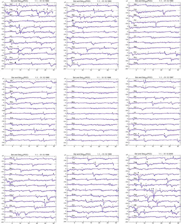
P. Stauning: J. Space Weather Space Clim. 2021, 11, 19

Troshichev & Andrezen (1985) was based on the magnitude (in           the mid-latitude Kp index, and ring current indices. Such
nT) of 15 min samples of the magnetic variation in the direction      comparisons have not yet been published.
of the 03:00–15:00 MLT meridian. The MAGPC index was                       A further prime objective is the clarification of the timing
introduced as a measure of the geo-effective interplanetary           and amplitude relations between polar cap indices (PC) and ring
electric field to be derived from available ground-based               current indices, in particular, the Dst index. Published relations
magnetic observations in the central polar caps.                      range from simplified rules for the timing and amplitude rela-
     A major problem for these initial “PC” indices was their         tions between maximum PC index values and negative peak
dependence on the daily and seasonal changes in ionospheric           Dst or SYM-H index values (e.g., Troshichev et al., 2011b;
conductivity with the varying solar illumination. These               Troshichev & Sormaov, 2018; ISO/TR/23989, 2020), to neural
variations would generate corresponding variations in the             network-based estimations of Dst values 1 h ahead from input
“sensitivity” of the response in the disturbance indices to vary-     of past 12 hours PCN and PCS values (Stepanova et al.,
ing solar wind conditions.                                            2005). The present approach makes it possible to derive precise
     The present version of the Polar Cap (PC) index is based on      and detailed ring current intensities by integration of a PCC-
the formulation by Troshichev et al. (1988). The new idea here        based source function from any quiet state (Dst  0) up to 45
is the scaling on a statistical basis of the magnetic variations to   min past actual time and marks a paradigm shift compared to
the electric field in the solar wind (Kan & Lee, 1979) in order to     previous efforts seeking direct relations between PC and
make the new PC index independent of local ionospheric prop-          SYM-H (or Dst) index values (e.g., relations between PC
erties and their daily and seasonal variations. For the calculation   maxima and Dst or SYM-H minima).
of PC index values they, furthermore, used magnetic variations             The polar cap indices, PCN and PCS, provide a great poten-
in an “optimal direction” perpendicular to the DP2 transpolar         tial for Space Weather monitoring and Space Weather-related
convection. The PC index concept was further developed by             research (e.g., Stauning et al., 2008; Stauning, 2012). The
Vennerstrøm (1991) and Troshichev et al. (2006).                      PCC index construction, as shall be shown, provides more accu-
     The standard Polar Cap (PC) indices, PCN (North) and PCS         rate estimates of the solar wind energy that enters the magneto-
(South) used also for the PCC index discussed here are derived        sphere than available from the individual PC indices or further
from polar magnetic variations recorded at Qaanaaq (Thule) in         combinations. A particularly important application is the use of
Greenland and Vostok in Antarctica, respectively. The introduc-       strongly enhanced PC index levels (Stauning, 2013c, 2020a) to
tion of the non-negative PCC index formed by combining PCN            predict violent substorm events that could threaten important
and PCS indices (Stauning, 2007) has resolved two conceptual          subauroral power grids (Kappenman, 2010).
dilemmas for the interpretation of PC indices assumed represen-
tative of the input of energy from the solar wind to the magne-
tosphere. One is the question of which one of the two                 2 Calculation of polar cap indices
hemispherical indices, which at times display considerable dif-
ferences, would provide the best representation of the incoming           The transpolar (noon to midnight) convection of plasma and
solar wind energy. The other dilemma is the problem that a con-       magnetic fields driven by the interaction of the solar wind with
siderable fraction of either index version, as shall be demon-        the magnetosphere generates electric (Hall) currents in the upper
strated, takes negative values. They would then represent             atmosphere in the opposite direction. These currents, in turn,
outflow of energy to the solar wind leaving the magnetosphere          induce magnetic variations at ground level (Troshichev et al.,
void of magnetic disturbances which could be true in some but         1988, 2006; Vennerstrøm, 1991). In order to focus on solar wind
far from all cases.                                                   effects, the horizontal magnetic variations, DF = F  FRL, of the
     The PC indices have been used in various versions in
                                                                      recorded horizontal magnetic field vector series, F, with respect
studies of the relations between polar cap disturbances and fur-
                                                                      to an undisturbed reference level, FRL, are projected to an
ther activity parameters such as solar wind electric fields, and
                                                                      “optimum direction” in space assumed perpendicular to the
magnetospheric storm and substorm indices. In de Campra &
                                                                      DP2 transpolar convection-related sunward currents. The opti-
de Artigas (2004), Gao (2012), Gao et al. (2012), Huang
                                                                      mum direction is characterized by its angle, u, to the dawn-dusk
(2005), Stepanova et al. (2005), the PCN version developed
                                                                      meridian and defines the direction for positive DFPROJ values.
by Vennerstrøm (1991) were used. Janzhura & Troshichev
                                                                      Next, the DFPROJ scalar values are scaled to generate a PC index
(2011) and Troshichev et al. (2011a) used PCN indices in the
                                                                      equal on the average to the solar wind merging electric field, EM,
AARI version while Troshichev et al. (2011b) implemented
                                                                      (also termed EKL) formulated by Kan & Lee (1979):
local summer selections of either PCN or PCS. Troshichev
                                                                                                            1=2
et al. (2012), Troshichev & Janzhura (2012), and Troshichev                        EM ¼ V SW  BY 2 þ BZ 2        sin2 ðh=2Þ       ð1Þ
& Sormakov (2019) used both the summer and winter index
selection while Troshichev & Sormakov (2015, 2018) used               where VSW is solar wind velocity, BY and BZ are Geocentric
the average of PCN and PCS indices to represent PC index              Solar-Magnetosphere (GSM) components of IMF, while h is
values in their work. In many calculations and illustrations          the polar angle of the transverse IMF vector.
presented in these publications, the index combination is just            The projected polar cap magnetic disturbances are assumed
named “PC index” and not further specified.                            proportional to EM:
     Thus, a prime objective for the present work has been to                              F PROJ ¼ a  EM þ b:                    ð2Þ
systematically compare the performances of the individual
(unipolar) PC indices and combinations such as non-negative           The PC index is now defined by:
or simple averages or seasonal selections used in correlation
studies involving the solar wind merging electric field, EM,                           PC ¼ ðF PROJ  bÞ=a ð EM Þ:                 ð3Þ

                                                              Page 2 of 23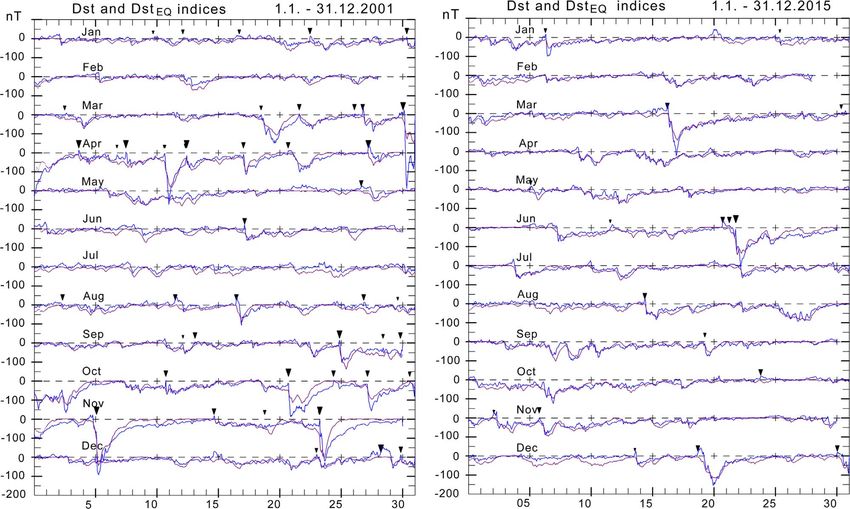
P. Stauning: J. Space Weather Space Clim. 2021, 11, 19

    The optimum angle, u, and the propagation delay, s,
between the reference location for the solar wind data and the
location for related effects at the polar cap are both estimated
from searching the optimum correlation between EM and
DFPROJ (e.g., Stauning, 2016). The correlation coefficient is
usually around 0.75 and the delay from Bow Shock Nose
(BSN) to the polar cap is close to 20 min. regardless of the
observatory positions in their daily rotation.
    The calibration constants, the slope, a, and the intercept, b,
are found by linear regression between samples of DFPROJ and
EM for each moment of the day and year using an extended
epoch of past data (Stauning et al., 2006; Troshichev et al.,
2006; Stauning, 2016). The regression parameters and the opti-
mum angle values are tabulated throughout the year at 1-min
resolution. They are kept invariant over years.
    During conditions where the IMF BZ component is negative         Fig. 1. Upper field: IMF BY (red line), IMF BZ (black, dots). Lower
or small, the forward convection (DP2) patterns prevail and          field: PCN (blue line), PCS (red), PCC (magenta, dots), and EM
generate positive DFPROJ values. The slope parameter (a) is          values (black) during 17 June 2015.
positive and the intercept term (b) is relatively small. Hence,
the PC index values (cf. Eq. (3)) are mostly positive. During
positive (northward) IMF BZ (NBZ) conditions, reverse convec-        In this case the mean of PCN and PCS would still be negative
tion patterns (DP3) may emerge and generate negative                 and quite large. During the interval of northward BZ (NBZ)
DFPROJ values which, in turn, may generate negative PC index         conditions with positive IMF BZ values and small EM values,
values.                                                              the PCC index values remain close to zero during the episode
    The PCC indices are derived from the mean of non-negative        of strongly negative PCN and small PCS values. Such events
values of the PCN and PCS indices:                                   occur most frequently during local midday hours in the summer
                                                                     season.
  PCC ¼ ðPCN if > 0 or else 0 þ PCS if > 0 or else 0Þ=2:                 The daily and seasonal variations in negative PC index
                                                              ð4Þ    values associated with negative values, DFPROJ < 50 nT, of
                                                                     the projected horizontal disturbance vector (cf. Eq. (3)) associ-
Thus, the PCC index values are always non-negative like the          ated with reverse convection conditions, are illustrated in
merging electric field, EM, used for the calibration of the indi-     Figures 2a and 2b. The 50 nT DFPROJ level corresponds to
vidual polar cap indices. The rationale behind this formulation      a PC index value of around 1 mV/m.
builds on a critical assessment of the consequences of negative          The differences between the two polar cap observatories are
index values. At negative PC index values in both hemispheres,       evident in Figures 2a and 2b. Figure 2a shows that the reverse
the global magnetic activity goes low like the PCC index             convection conditions mainly occur at around 16 UT for
values. A positive PC index in one hemisphere indicates unipo-       Qaanaaq, which is close to local noon whether in geomagnetic
lar solar wind energy entry and generation of global magnetic        or geographic time. For Vostok, geomagnetic and geographic
disturbances in agreement with the positive PCC index values         noon are more separated, which generates the double-peak
even if the PC index for the other hemisphere is dominatingly        structure in the daily variation. For the yearly variation both
negative.                                                            observatories display clear local summer maxima. The total
    It should be noted that the calculations of PCN and PCS          reverse convection intensities are significantly different for the
index values applied here differ from the IAGA-recommended           two observatories. The reverse convection intensities summed
methods with respect to the handling of reverse convection           over the years 1997–2009 amounts to 2.2  105 nT hours
samples and reference level construction. This issue is discussed    for Qaanaaq and 0.74  105 nT hours for Vostok as noted
in Section 7.                                                        in the diagrams of Figure 2 (Stauning, 2015). This difference
                                                                     has a significant impact on the symmetry of index scaling
                                                                     parameters and index values for the two unipolar PC indices.
                                                                         With forward convection cases with positive values,
3 Occurrences of negative PCN and PCS                                DFPROJ > 50 nT, of the projected horizontal disturbance vector
  index values                                                       during the same span of years (1997–2009), the total convection
                                                                     intensities amount to around 2.5  106 nT hours for both
    The occurrences of negative values of the projected mag-         observatories (Stauning, 2015). Thus, on the average, reverse
netic disturbances (reverse convection) and their adverse effects    convection intensities are around 10% of the forward
on calculations of index calibration parameters were discussed       convection integrated intensities for Qaanaaq and only 3% for
in Stauning (2013a, 2015). Figure 1 displays an example of           Vostok. For both observatories, the relative amounts of reverse
negative PCN values.                                                 convection cases are significantly higher at midday in the
    Note in Figure 1 the strongly negative values of PCN             summer season compared to different local hours and seasons.
following the abrupt IMF turning northward to make                   For Qaanaaq the peak reverse convection intensities
BZ  +4 nT shortly after 15 UT close to local noon (16 UT            (cf. Figs. 2a and 2b) are around 4  103 nT hours/h during
at Qaanaaq) while the PCS indices are close to zero at this time.    summer daytime conditions while the forward convection at

                                                             Page 3 of 23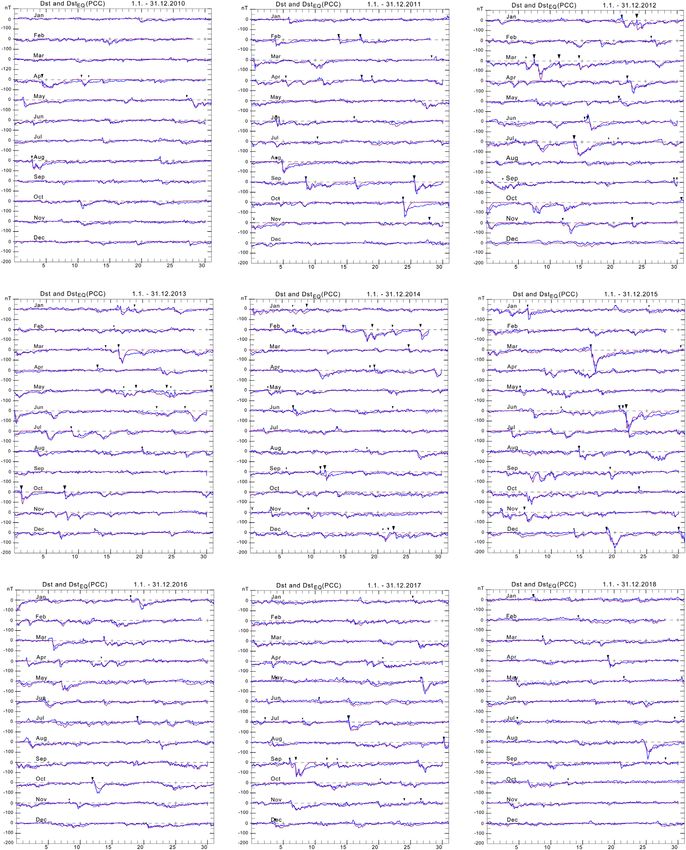
P. Stauning: J. Space Weather Space Clim. 2021, 11, 19

(a)                                                                  (a)

(b)
                                                                     (b)

Fig. 2. (a) Average daily and (b) average seasonal variations in
reverse convection intensities for Qaanaaq (THL) (blue line) and     Fig. 3. Display of hourly values of the X and Y components of
Vostok (red) defined by the hourly product of amplitude (in nT) and   magnetic data from Qaanaaq (THL) and Vostok (VOS) using fixed
duration (hours).                                                    base line levels (Xbl, Ybl) throughout the 3 years.

summer daytime is around 1.5  104 nT hours/h. Thus the              problem for the magnetometer data reported to Intermagnet as
peak reverse convection intensities are around 25% of the for-       seen in Figure 3b. Both diagrams use fixed base level values,
ward convection intensities for Qaanaaq, while for Vostok the        Xbl, Ybl, throughout the 3 years of displayed data.
reverse convection intensities are only around 6% of the                 As part of the processing prior to PC index calculations,
forward convection intensities during local summer daytime           the baseline values have been adjusted to present smooth
conditions.                                                          (secular) variations throughout the span of years included in
                                                                     the epoch from 1992 to 2018. The derived PCN and PCS values
                                                                     have, furthermore, been visually scanned (and compared to each
                                                                     other) in order to detect irregular index behaviour like the
4 Relations of PCN, PCS and PCC to the                               erroneous daily excursions in the AARI PCS indices for 2011
  merging electric field, EM                                         seen in Figure 16 here (cf. Stauning, 2018a, 2020b).
                                                                         Results from the correlations of PC index values in different
    The relations of the polar cap indices, PCN, PCS and PCC         versions with values of the merging electric field are displayed
to the merging electric field, EM (Eq. (1)), in the impinging         in Figures 4–6.
solar wind have been investigated for the span of years from             The correlation coefficients, Rx, have been derived on a
1992 to 2018. The magnetic data supplied from Intermagnet            seasonal basis for the display in Figure 4. Spring values plotted
(https://intermagnet.org) for Qaanaaq (THL) and Vostok have          at mid-March are the results from successive February, March,
been supplemented since 2009 by data from Dome-C observa-            and April data and so on. The coefficients for the correlation
tory in Antarctica (Chambodut et al., 2009; Di Mauro et al.,         between PCN and EM are displayed in blue line, The PCS –
2014). All index values have been derived by using the DMI           EM correlation in red, while the PCC – EM correlation coeffi-
index calculation methods and coefficients (Stauning, 2016).          cients are shown in heavy magenta line. The PCC indices were
Figures 3a and 3b display hourly values of the X and Y compo-        in most cases derived from Qaanaaq-based PCN and Vostok-
nents of the magnetic recordings from Qaanaaq operated by the        based PCS values. For the years 2012 and 2013 where the
Danish Space Research Institute (DTU Space) and from Vostok          Vostok data were incomplete, data from Dome-C (DMC) obser-
operated by the Arctic and Antarctic Research Institute (AARI)       vatory were used to derive an alternative PCS index, here
in St. Petersburg. Special care for index calculations was given     denoted PCD. The correlation between EM and PCD is dis-
to data from Vostok since there is, apparently, a base level         played in green line, while the correlation between EM and

                                                             Page 4 of 23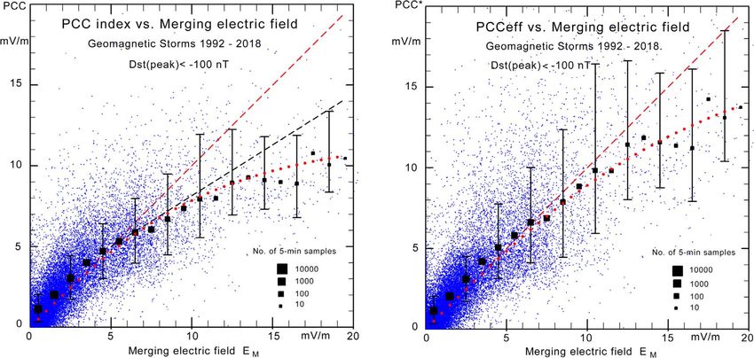
P. Stauning: J. Space Weather Space Clim. 2021, 11, 19

                                                                        Fig. 6. Display of monthly average coefficients for the correlation
                                                                        between EM and PCN(blue line), PCS (red), and PCC (magenta).

Fig. 4. Correlation of the solar wind merging electric field, EM, with
polar cap indices, PCN (blue line), PCS (red), PCC (magenta), PCD
                                                                        months, November–January, for Vostok than for the other
(green), and PCCD (black). PCD and PCCD use Dome-C magnetic
                                                                        seasons. Selecting the local winter index, PCW, that is, jumping
data.
                                                                        between the PCN and PCS traces, improves correlation values
                                                                        while selecting the local summer index (PCU) reduces correla-
                                                                        tions. It is seen that the correlation between PCC and EM is low-
                                                                        est during the northern winter months (November–January).
                                                                        However, the overall correlation between PCC and EM is clearly
                                                                        higher throughout all years and all seasons than the correlations
                                                                        between EM and either of PCN, PCS, PCA (average of PCN
                                                                        and PCS), PCW, and PCU index versions. From Figures 4
                                                                        and 5 there is a tendency for decreasing correlations between
                                                                        EM and either of the PC indices with time over the recent years.
                                                                        However, an in-depth investigation of this issue is beyond the
                                                                        scope of the present submission. Correlation coefficient values
                                                                        for the unipolar PC indices and their combinations throughout
                                                                        the available spans of years are displayed in Table 5 of the
Fig. 5. Yearly averages of correlations between EM and PCN (blue        summary Section 8.
line), PCS-Vostok (red), PCS-Dome-C (green), PCC-(Qaanaaq-
Vostok) (heavy magenta), and PCCD-(Qaanaaq-Dome-C) in heavy
black line.                                                             5 Relations between the PC and Kp indices

                                                                            The added amount of polar magnetic data available now
PCC derived by using PCN and PCD values is displayed in                 (2020), among other from the Dome-C observatory, compared
heavy black line (PCCD).                                                to the situation in 2007 where the PCC index concept originated
    It is readily seen from Figure 4 that the correlation between       (Stauning, 2007), and in 2008 and 2012 where the PCC index
PCC and EM is significantly higher than the correlation between          concept was further developed (Stauning et al., 2008; Stauning,
either of PCN or PCS and EM. It is also seen that the correlation       2012), makes it worthwhile to re-examine relations between the
between PCN and EM, in most cases, is lower than the correla-           PCC indices and other ground-based magnetic indices. Here,
tion between PCS and EM.                                                the mid-latitude Kp indices and the ring current indices derived
    The yearly correlation coefficients are presented in Figure 5.       from near-equatorial magnetic observations are considered.
Here, the correlations between PCS indices based on Dome-C                  The local K magnetic disturbance indices and, in particular,
data and EM are displayed for the full range of available data          the planetary Kp indices are to a large extent used in space
(2010–2018) in the green line while the coefficients for the             weather monitoring and solar-terrestrial research to provide indi-
correlation between PCCD based on PCN-PCD values and                    cations of the level of geomagnetic disturbances (Bartels, 1957;
EM are displayed in black line.                                         Menvielle et al., 2011). A problem for many applications of the
    Finally, in the series of displays of correlation coefficients,      K (and Kp) indices is their sparse 3-hour sampling rate. This
Figure 6 displays the monthly correlation coefficients based             limited accessibility could be contrasted to the 1-min availability
on values from the years 1998–2018 except 2003 void of                  of the PC indices that may provide almost instantaneous indica-
PCS data and 2013 with incomplete PCS data. Values for                  tions of the geomagnetic disturbance level. Thus the PC indices
Dome-C available since mid 2009 only are not included here.             might add to the timely surveillance of space weather conditions
    It is seen from Figure 6 that the correlations between PCN          otherwise provided more sparingly by the K (and Kp) indices.
and EM are clearly lower in the northern summer months, May–            With the PCN and PCS indices, the occasional occurrence of
July, than for the rest of the year. Similarly, the correlations        negative values is a conceptual problem since there is no unique
between PCS and EM are clearly lower in the local summer                relation between their values, when negative, and the K (or Kp)

                                                                Page 5 of 23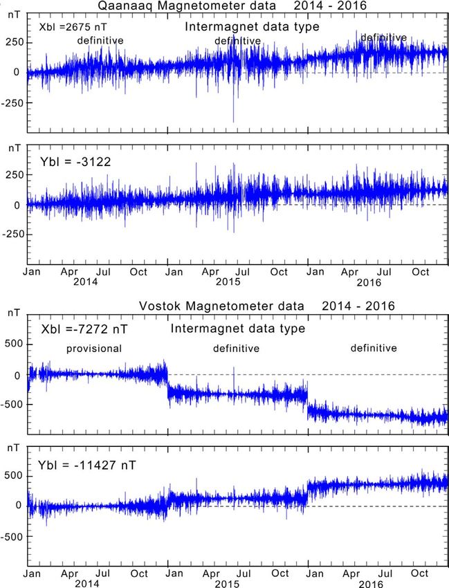
P. Stauning: J. Space Weather Space Clim. 2021, 11, 19

           (a)                                                      (b)

Fig. 7. Relations between Kp and the polar cap PCC indices. (a) Display of all KP-PCC samples. (b) Display without samples. The black
squares present averages of Kp index values and number of 15-min PCC samples for each unit of PCC while the error bars indicate standard
deviation. The dashed line indicates a linear relation while the small red dots indicate a functional relation.

indices. The use of the PCC indices improves the relation mak-        and regression results are presented in Table 1. All versions
ing it unambiguous and consistent as shown in Figure 7.               comprise the same number (53,414) of 3-h samples with the
    Figures 7a and 7b display the relation between Kp indices         requirement that valid PCN and PCS values should both be
represented on a triple fraction scale (Kp(0o) = 0.00, Kp             present.
(0+) = 0.33, Kp(1) = 0.67 and so on) and PCC index values                It is evident from the displays in Figures 8a–8d that there is
averaged over a 3-hour interval. Figure 7a displays the individ-      a problem with the negative PC index values for the interpreta-
ual Kp-PCC samples by short bars. The black squares present           tion of the Kp-PC index relations for all the displayed versions.
averages of Kp indices for each unit of PCC with the involved         Values of the correlation coefficients and results from the
number of 3-h Kp-PCC samples indicated by their size on the           regression based on 3-h samples throughout the epoch 1998–
lower right scale and with error bars to indicate standard            2018 are shown in Table 1 including the summer selection
deviation (spread). The red dashed line displays the slope and        indices (PCU). For uniformity, all parameters refer to the
intercept values derived from linear regression of Kp on PCC          no-delay cases.
(Kp as a function of PCC) with Kp being values on the regres-
sion line with slope S  1.00 (cf. Table 1). The PCC-based Kp
regression line provides a fair approximation up to Kp  5 but        6 Relations between PCC indices
clearly fails at larger PCC values.                                     and the ring current indices
         Kp ¼ Kp0 þ S  PCC
                                                              ð5Þ         The currents encircling the Earth near equator at distances of
            PCC in mV=m; S ¼ 0:987; Kp0 ¼ 0:847:                      typically 4–6 Re could be divided into the symmetrical part
                                                                      (RCS) formed all the way around the Earth, mostly by drifting
The small red dots indicate the least squares best fit between the     mirroring energetic electrons and ions, and the partial ring
3-hourly Kp and PCC values and a functional relation of the           current (RCP) mainly developing at the night side only. The
form:                                                                 ring current intensities are detected from a network of near-
   Kp ¼ Kp0 þ PCC  ð1 þ ðPCC=PCC0 Þ2 Þ
                                               1=2                    equatorial magnetometer stations and processed at World Data
                                                              ð6Þ     Centre WDC-C2 in Kyoto to provide indices for the symmetri-
     PCC in mV=m; PCC0 ¼ 10  mV=m; Kp0 ¼ 0:80:                      cal as well as the partial ring currents (Sugiura & Kamei, 1981).
                                                                      The hourly average symmetrical deflections scaled from the
The function has no direct physical origin but has been included      horizontal (H) components define the Dst indices. The corre-
to illustrate the systematic relation between Kp and PCC includ-      sponding symmetrical ring current index scaled from 1-min
ing the saturation effects at enhanced disturbance levels. For        values of the H and D components provides the SYM-H and
small PCC values, equations (5) and (6) provide nearly the same       SYM-D indices, respectively. Similarly, the asymmetrical parts
results. Equation (6) should be used for calculations of equiva-      of the 1-min H and D components generate the ASY-H and
lent Kp indices from observed PCC values in order to avoid            ASY-D indices.
unrealistic high Kp index values above 90 for PCC above 8
mV/m.                                                                 6.1 Asymmetrical ring current index, ASY-H
     The correlation between Kp and PCC for the cases presented
in Figure 7 has a value of Rx = 0.815 with no delay between the           The asymmetrical ring current indices, ASY-H, are provided
index series. Stepwise shifting the PCC timing up and down (in        by Kyoto WDC-C2 (Iyemori et al., 2000) as 1-min values. For
steps of 2 min) has demonstrated that the delay = 0 provides          the present statistical study a less detailed time resolution is con-
optimum correlation. The corresponding displays for other PC          sidered appropriate. Hence, the ASY-H indices and the polar
index versions are shown in Figures 8a–8d while the correlation       cap indices, PCC, have been averaged to form 15-min samples.

                                                             Page 6 of 23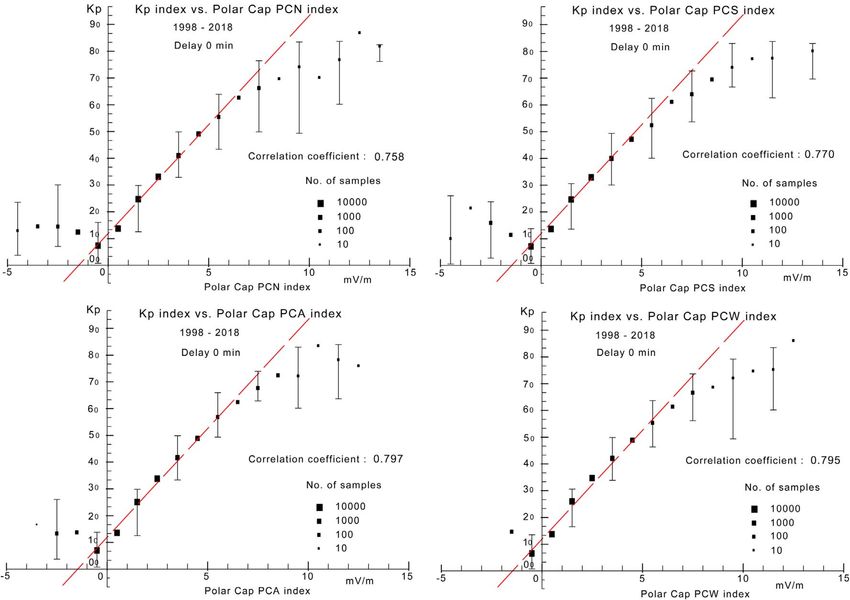
P. Stauning: J. Space Weather Space Clim. 2021, 11, 19

Table 1. Correlation coefficients and regression results for Kp-PC relations. Epoch 1998–2018.

Parameter                  PCC              PCN              PCS               PCA1)           PCW2)             PCU3)               mV/m
Correlation               0.815            0.758            0.770              0.797            0.795             0.736
Slope (S)                 0.986            0.813            0.843              0.903            0.902             0.764            (mV/m)1
Intercept (Kp0)           0.847            1.122            1.052              1.025            1.021             1.145

1)
     Average of available PCN and PCS values.
2)
     Winter values of PCN or PCS index values.
3)
     Summer values of PCN or PCS index values.

             (a)                                                        (b)

             (c)                                                        (d)

Fig. 8. Display of Kp against PCN (a), PCS (b), PCA (c) and PCW (d) in the format of Figure 7b. The dashed red lines are illustrative only and
placed to fit the positive PC index values. Note the upturns for negative PC index values.

The 15-min index data sets have been subjected to linear corre-          the figure was found to provide least RMS deviation and opti-
lation analyses using a stepwise variable delay between samples          mum correlation (Rx = 0.743) for 15-min samples of the two
of the respective time series assuming that the maximum value            index series. A noteworthy feature in the display is the persistent
of the correlation coefficient provides the most appropriate              close linear relations between the average ASY-H values and
delay. With this delay imposed on all pairs of samples of the            PCC indices up to high disturbance levels reflected in both
time series, a linear relation between the two parameter sets            indices. The regression and correlation were based on using
was found by least squares regression analysis. The average              all available ASY-H – PCC sample pairs (around 30,000).
deviation, the average numerical (absolute) deviation, and the           The relation is expressed below:
RMS standard deviation, were calculated from the assumed
linear relations.                                                                        ASYH ¼ 10:9  PCC þ 16 ½nT:                     ð7Þ
     The present investigation has considered 4-days intervals
from most major geomagnetic storms with Dst(peak) < 100 nT              Studies of the correlation between ASY-H and PC indices may
occurring between 1992 and 2018 with the onset occurring on              also be used to look at the relevance of further PC index
the first day. Figure 9 displays scatter plots of 15-min ASY-H            versions in play. It has been claimed (Troshichev, 2017; ISO/
index values against PCC values. The 8 min delay noted in                TR/23989, 2020) that either of the unipolar indices with the

                                                                Page 7 of 23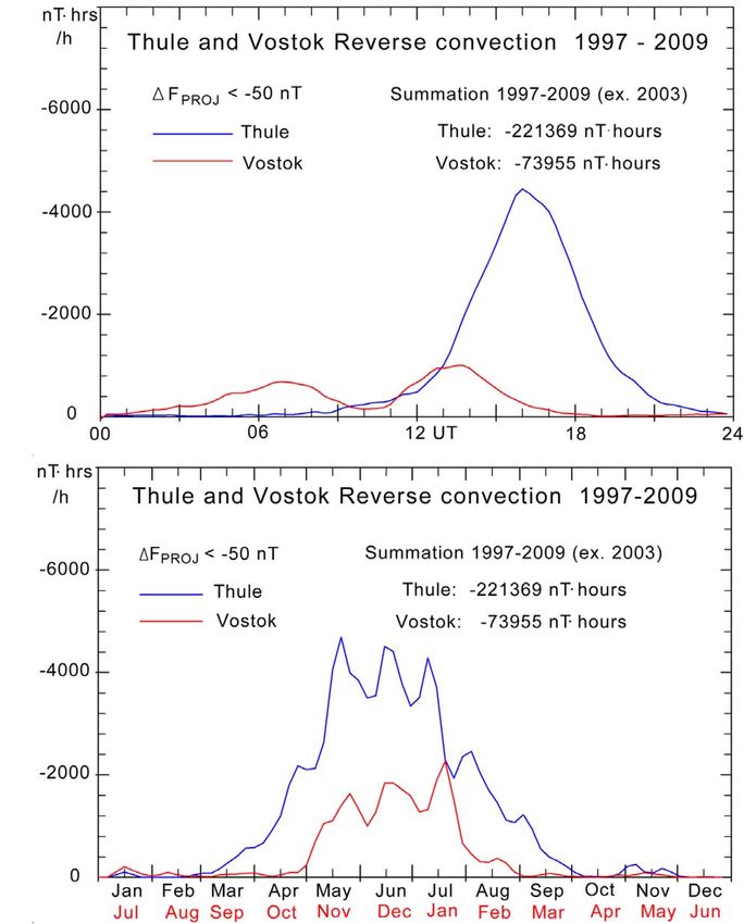
P. Stauning: J. Space Weather Space Clim. 2021, 11, 19

           (a)                                                          (b)

Fig. 9. Scatter plots of ASY-H against PCC index values. (a) Display of individual ASY-H-PCC samples. (b) Display without samples. The
black squares indicate average values and number of 15-min samples within each unit interval in PCC, while the error bars at every other unit
interval indicate standard deviation. The red dashed lines indicate least squares regression on the 15-min data samples (Eq. (7)). Note the good
fit to the interval-average squares.

     (a)                                                                (b)

     (c)                                                                (d)

Fig. 10. Displays corresponding to Figure 9b for the relations between ASY-H and PC indices represented by (a) PCN, (b) PCS, (c) PCA
(average of PCN and PCS), and (d) winter hemisphere PCW index. The red dashed lines are illustrative only and placed to fit the positive PC
index values. Note the upturns for negative PC index values.

adjustments of the reference level (QDC) to include a solar wind          criteria (magnetic storm intervals). Hence no effort was made to
sector term would provide an adequate representation of the               avoid intervals where data for one or the other index version
solar wind effects on the magnetosphere. In further publications,         were missing.
Troshichev et al. (2012) have used the seasonal selections of                  It is readily seen from Figures 10a–10d that the data for the
summer PC indices in their investigations of the relations                positive averages of index values are well represented by a lin-
between PC and ASY-H indices. The results from the examina-               ear approximation corresponding to equation (7). The problems
tion of the PC-ASY-H relations using the various versions are             reside, in particular, with the negative PC index values. While
displayed in the diagrams of Figures 10a–10d and in Table 2.              the correlation coefficient for 15-min samples of the PCC-
    It should be noted that data for the various versions have            ASY-H relation in Figure 9 is Rx = 0.74, then the correlation
been selected from the epoch 1992–2018 on basis of the same               between the ASY-H and PC indices for the cases presented in

                                                                 Page 8 of 23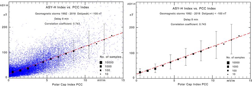
P. Stauning: J. Space Weather Space Clim. 2021, 11, 19

Table 2. Number of samples, correlation coefficients, and regression results for ASY-H/PC relations.

Parameter             PCC               PCN               PCS               PCA              PCW               PCU                 Unit
Samples              28,803            34,839            28,802            28,880           33,728            29,913
Correlation           0.743             0.702            0.679              0.716            0.700            0.683
Slope                 10.9               9.5              9.5               10.1              9.7              9.7             nT/(mV/m)
Intercept              16                 27               27                32                30               20                 nT
Mean dev.             1.7              0.3              0.8              0.5              0.1              0.6                nT
RMS dev.              23.6              24.5              25.6              24.0              24.0             25.5                nT

Figures 10a–10d (including summer indices, PCU) are all close
to a correlation coefficient value of Rx = 0.70. The number of
15-min samples, correlation coefficients and results from the
linear regression analyses are summarized in Table 2.

6.2 Symmetrical 1-min ring current index, SYM-H

     The 1-min symmetrical ring current index, SYM-H, can be
exposed to a correlation and regression study equivalent to the
study presented in Section 6.1 for the ASY-H index. Results
from such studies are displayed in Figure 11 with the delay
set to 60 min (PCC leading over SYM-H).
     With the SYM-H, contrary to the ASY-H index, the corre-            Fig. 11. Scatter plots for SYM-H vs. PCC in the format of Figure 9b
lation with PCC does not provide a clear maximum, but contin-           with delay 60 min.
ues to increase very slowly with increasing delay up to more
than 3 hours. With increasing delays, the correlation coefficient
increased from Rx(0h) = 0.533 to Rx(1h) = 0.623, Rx(2h) =
0.636, and Rx(3h) = 0.645. The explanation is probably that             provided in Jorgensen et al. (2004) are used here, while the
the large PCC values at the start of the events correlate well with     decay function provided by Feldstein et al. (1984) is used for
large slowly varying SYM-H values recorded through many                 the loss term in the first step. This function uses two decay time
hours of the continued ring current build-up. Thus, the direct          constants, s = 5.8 h for large disturbances where Dst < 55 nT,
correlation of the symmetrical ring current indices with PC             and s = 8.2 h for small disturbances where Dst > 55 nT. Now,
indices is not meaningful beyond the simple conclusion that             the relation in equation (8) has only terms relating to the source
large PC index values relate to large SYM-H index values.               function Q and may provide derived Dst index values by
                                                                        integration from a known state, once the source term is defined.
6.3 Hourly ring current index, Dst                                          In Burton et al. (1975) the source term Q was related to the
                                                                        YGSM component of the solar wind electric field. In the analyses
    The failure of reaching maximum correlation between PCC             by Stauning et al. (2008) and Stauning (2012), the relations of
and the symmetrical 1-min ring current index, SYM-H also                Q to the polar cap indices were examined for a number of storm
includes the Dst hourly ring current index. The approach                event cases during the interval 1995–2002 and 1995–2005,
suggested in Stauning et al. (2008) and Stauning (2012) has             respectively. Here we repeat these analyses using in the first step
been applied instead. Thus, the PCC index is used in a source           selected large storm events throughout 1992–2018 in order to
function to describe the gradient in the Dst index rather than          improve the statistical basis. In 4-days segments of all
in correlations with its actual value.                                  selected storm cases with Dst (peak) < 100 nT and storm
    The Dst index is considered to represent the energy stored in       onset on the first day, we first derive the temporal change at
the ring current. With Dst* being the recorded Dst index                time t = T in the hourly Dst* index from the hourly values at
corrected for contributions from magnetopause currents                  t = T  1 and t = T + 1 [h] by the simple differential term:
(MPC) mostly related to the solar wind dynamical pressure, a
relation between the accumulated kinetic energy of the charged            dDst =dt ðT hÞ ¼ ðDst ðT þ 1 hÞ  Dst ðT  1 hÞÞ=2: ð9Þ
particles encircling the Earth and the Dst* index is provided by
the Dessler-Parker-Sckopke relation (Dessler & Parker, 1959;            In order to derive the source function, Q, to be used in equation
Sckopke, 1966). Following Burton et al. (1975), the rate of             (8), the average slope values defined by equation (9) are
change in the Dst* index with time could be written:                    corrected by including the decay term defined above using the
                                                                        current Dst* value at t = T. For the amount of archived geomag-
        dDst =dt ½nT=h ¼ Q½nT=h  Dst ½nT=s ½h:           ð8Þ     netic storm data, the resulting source function, QOBS, is then
                                                                        related to the PC indices considered being potential source
The quantity Q (in nT/h) is the source term while the last term in      parameters since they relate to the interplanetary electric field
equation (8) is the ring current loss function controlled by the        albeit in the Kan & Lee (1979) version and not the YGSM-
decay time constant, s, here measured in hours. For the small           component used by Burton et al. (1975). Variable positive or
actual MPC corrections, the Dst dependent statistical values            negative delays were imposed on the relation. The PCC indices

                                                                Page 9 of 23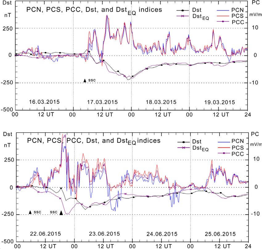
P. Stauning: J. Space Weather Space Clim. 2021, 11, 19

                                                                        importance for the relations between Dst and its possible source
                                                                        functions, primarily the PCC index. A further parameter intro-
                                                                        duced here is the optimum delay between samples of the
                                                                        PCC time series and the calculated Dst values. For these cases,
                                                                        the PCC-based index values lead by a few (45) minutes.
                                                                            In addition to the decay time constants (Feldstein et al.,
                                                                        1984) and delays, the examination has included the impact from
                                                                        the saturation of the PC indices for high levels of the merging
                                                                        electric field (e.g., Stauning, 2018a). In Figures 13a and 13b
                                                                        the individual 15-min samples are displayed by the small blue
                                                                        dots. Bin-average values are displayed by the black squares
                                                                        sized to indicate the number of 15-min samples on the lower
Fig. 12. Scatter plot of d(Dst*)/dt corrected for decay vs. polar cap   right scale. Error bars display standard deviation. The dashed
PCC index. The black squares represent bin-average values and no of     red line indicates equality between PCC and EM.
hourly samples while the error bars in every other bin represent            Figure 13a indicates that the PC indices saturate at high
standard deviation among samples.                                       levels of EM. The systematically positioned red dots display a
                                                                        functional relation between PCC and EM regulated by the
                                                                        asymptotic parameter, E0 derived by least squares regression
are provided here at a more detailed time resolution (5 min) than       between interval-average values (black squares) and the regres-
the hourly source function values. By shifting the averaging            sion curve (Stauning, 2012):
interval by delays varying on a 5-minute scale, hourly averages                                                         1=2
of the parameters are correlated with the hourly source function                       PCC ¼ EM  ð1 þ ðEM =E0 Þ2 Þ            :        ð11Þ
values to derive the delay that produces the maximum correla-
tion through the ensemble of storm events. With this delay the          Note that this functional relation is just used for visual indication
best fit linear relation between the source function values and          of the saturation problem.
the relevant source parameter is determined by the linear regres-           In a crude approximation for the parameter iteration process,
sion analysis illustrated in Figure 12.                                 the effective PCC indices (PCCeff) are set equal to the EM values
    In Figure 12, hourly values of dDst*/dt corrected for decay         up to a turning level (PCClim) at around 5 mV/m and then
have been plotted against the related PCC index values.                 forced to deviate by adding a linear relation with slope (S) less
Average values within each unit of PCC are displayed by the             than unity. The approximation is defined by the two-step linear
black squares with sizes corresponding to the number of hourly          relation in equations below:
samples according to the lower right scale.
                                                                           PCC ¼ EM       for PCC < PCClim ðPCClim ¼ EMlim Þ          ð12aÞ
    The scatter plot in Figure 12 presents the Dst* source func-
tion, QOBS, based on observed hourly Dst values corrected for           and
decay (Feldstein et al., 1984) plotted against the polar cap index,
PCC, considered to be a potential source parameter. The relation            PCC ¼ EMlim þ S  ðEM  EMlim Þ        for PCC > PCClim :
between the best fit source function, QOBS, and the source                                                                             ð12bÞ
parameter values, PCC, is then expressed in a linear function.
From the present data set (98 storm periods 1992–2018) we               Conversely, an “effective” PCC index could be defined to pro-
obtain by regression on the total amount of hourly samples:             vide a value equivalent to EM in its effect on the energy transfer
                                                                        to the magnetosphere by equations below:
       QOBS ½nT=h ¼ 4:1 ½ðnT=hÞ=ðmV=mÞ
                                                                                      PCCeff ¼ PCC       for PCC < PCClim             ð13aÞ
                         PCC ½mV=m  2:2 ½nT=h:              ð10Þ
                                                                        and
Further versions of the analysis displayed in Figure 12 have
been performed with stepwise variable delays to reach an opti-                PCCeff ¼ PCC þ ð1=S  1Þ  ðPCC – PCClim Þ
mum correlation R = 0.668 at a delay of DT = 15 min with PCC                                                                          ð13bÞ
                                                                                for PCC > PCClim
leading.
    This result is close to the corresponding source function           where Seff = 1/S  1 is less than unity.
(Q = 4.6  PCC  1.2) defined in Stauning (2012) from a                     The black dashed line in Figure 13a displays equations
smaller amount of data (storm events 1995–2005).                        (12a) and (12b) with EMlim ¼ 5 mV=m and S = 0.63 while
    With continuous time series of the PCC-based source                 Figure 13b displays the individual and average PCC values as
values, and specification of the relational constants and initial        well as the fitted function modified by equations (13a) and
Dst values, it is now possible, at least in principle, to integrate     (13b) with EMlim = PCClim = 5 mV/m and Seff = 0.60.
equation (8) to derive values of an “equivalent” Dst index,                 A test bed to handle multiple parameter adjustments is pro-
DstEQ, throughout any interval of time. The present work has            vided by the above-mentioned set of 98 magnetic storms with
brought the analysis of the relations between Dst and the polar         peak Dst below 100 nT occurring throughout the epoch from
cap index, PCC, important steps forward compared to Stauning            1992 to 2018 where PCS indices are available (with some gaps).
(2012) by including a close examination of the Feldstein et al.         For calculation of PCN indices, Qaanaaq (THL) data are
(1984) decay time constants (s = 5.8 h and s = 8.2 h) and their         virtually continuously available since 1975. Vostok magnetic
turning level (Dst, lim = 55 nT), and other parameters of              data were not available for PCS calculations during most of

                                                                Page 10 of 23
P. Stauning: J. Space Weather Space Clim. 2021, 11, 19
(a) (b)
Fig. 13. (a) Relations between the merging electric field, EM, and the polar cap, PCC, index. The small blue dots display the individual 15-min
samples. The larger black squares with error bars show the bin-average values and sample numbers. The dashed red line indicates equality
while the red dots display a functional relation between EM and PCC. The dashed black line indicates a PCC modification (b) Same data set but
with the modified PCC values (PCCeff) displayed against EM.
1993 and 1996, all of 2003, and parts of 2012 and 2013. (a)
Dome-C magnetic data have been substituted for missing or
unreliable Vostok data for PCS calculations throughout 2012
and 2013. For each storm event a sequence of 4 days is
considered with the storm starting on the first day. Starting on
the initial values defined in Feldstein et al. (1984), the parame-
ters have been changed in small successive step searching for
maximum correlation and minimum deviations.
Examples of observations-based and equivalent Dst values
are displayed in Figures 14a and 14b. For these cases the inte-
gration of the source term has been started at the real Dst value (b)
and then allowed to proceed independently throughout the 4
days in each set.
The examples in Figures 14a and 14b represent cases of
good correlation (Rx = 0.957) and poor correlation (Rx =
0.762) compared to the average correlation level (Rx = 0.810,
cf. Table 4). Note also in Figure 14b the intervals of strongly
negative PCN values which, if included, would decrease the
correlation between the published (real) Dst and the PCC-based
DstEQ values considerably. A further feature of Figure 14b is the
effects of the strong storm sudden commencement (SSC) at
15 UT on 22 June 2015. The SSC event not included in the
Dst modelling counteracts the PCC effects and prevents Fig. 14. (a, b) Examples of published (real) Dst (black line, dots) and
Dst from reaching the negative peak value displayed by the equivalent Dst (magenta, crosses) values calculated from the PCC-
DstEQ course. based source function. Values of PCC (magenta), PCN (blue), and
Figures 14a and 14b indicate good and fair agreement, PCS (red) are displayed in the upper fields on the right scale.
respectively, between the observed and the equivalent Dst
values. Generally, the agreement is best for moderate storms.
Going from the moderate to the strong storm cases gives With the understanding of the effects of adjustments of the
sometimes less agreement between real Dst values and equiva- various parameters gained from the test bed exercises, the full
lent PCC-based DstEQ values, possibly related to saturation range of available data has been used to integrate the PCC-
effects not compensated for by the PCC modifications defined based source function throughout 1992–2018 to derive equiva-
in equations (12a), (12b) and (13a), (13b). For the very weak lent DstEQ values without attachment at all to the published
cases the uncertain effects from magnetopause currents (real) Dst values. In the first step, the timing parameters have
(MPC), although small, may have relatively large effects. been adjusted to provide the overall best correlation and least
Page 11 of 23P. Stauning: J. Space Weather Space Clim. 2021, 11, 19
deviations. In the second step, the PCC high-level modification Table 3. Parameters for DstEQ calculations.
suggested in equations (13a) and (13b) has been used to provide
the best possible agreement between peak values of DstEQ and Symbol Fldst. PCC Test bed Optimal all Unit
Dst keeping the other parameters near their initial values. Fast decay, s1 5.8 6.5 5.5 h
The resulting iterated optimum parameters are presented in Slow decay, s2 8.2 7.0 7.0 h
Table 3 along with the original values used in Stauning (2012) DstX level 55 70 52 nT
while Table 4 presents the resulting quality control results. The Dst gradient 4.6 4.5 4.5 (nT/h)/(mV/m)
iterations gave slightly different parameters depending on which PCClim – 5.0 5.0 mV/m
of quality parameters being considered in the process. Thus, the PCCslope, Seff – 0.40 0.60 –
Delay DstEQ–Dst 0 45 45 min
parameter values of Table 3 are not unique but present
compromises.
The calculated DstEQ values are based on integration of the
source function defined from the PCC indices. In cases where
either PCN or (Vostok or Dome-C-based) PCS values were Table 4. Results from DstEQ calculations.
unavailable, the available hemispherical PC indices were used
Result term Fldst. PCC Test bed Optimal Unit
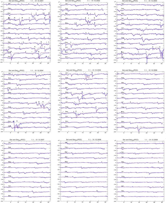
for PCC. The derived DstEQ values have been displayed in plots
along with the real Dst values throughout the entire epoch for Mean Dst 13.08 58.2 13.08 nT
control of the calculations. These plots are presented in the Mean DstEQ 15.90 58.1 13.09 nT
Appendix. Examples for the stormy years 2001 and 2015 are Mean diff. 2.83 0.11 0.01 nT
displayed in Figures 15a and 15b. Abs. diff. 9.37 23.12 8.88 nT
Figures 15a and 15b display close, although not perfect, RMS diff. 12.83 28.81 12.30 nT
Correlation 0.849 0.810 0.856
matches between the real Dst values (blue line) based on
observed near-equatorial magnetic variations and the equivalent
DstEQ values (magenta line) calculated by integration of the
PCC-based source function (Eq. (8)) using the parameters from
Table 3 including high-level modifications of the PCC indices. For the PC-Kp correlations, samples were formed by
The integration was performed in steps of 5 min starting from averaging PC indices over every time-shifted 3- h Kp interval.
DstEQ = 0 on 1 January 1992. Correlations and linear regressions were applied to these
In Tables 3 and 4 the column “Fldst. PCC” relates to samples. For use in text books’ standard formulas for correlation
the DstEQ calculations using the control parameters from and regression, the summation terms, typically, have the form
Feldstein et al. (1984) presented in Stauning (2012) and used shown here for the Kp-PC cross products:
with the PCC-based source function. The columns “Test
RXY ¼ R R RKpðn3h; nd; nyÞ PCAVR ðn3h; nd; nyÞ
bed” refer to the selection of 98 major storm event periods
(Dst(peak) < 100 nT), while the “Optimal” columns refer to ny ¼ 1998–2018; nd ¼ 1–365; n3h ¼ 1–8:
the total 1992–2018 sequence. ð14Þ
With this formulation the total number of Kp-PC samples is:
N = 20 years/epoch 365.25 days/year 8 3-h-intervals/day =
7 Discussions 58,440 samples. The interval-average numbers of these sam-
7.1 Correlation techniques ples are implemented in the sizes of the black squares referring
to the lower right (logarithmic) scale. Thus, the interval-average
In the present manuscript, all correlations are made by using squares display the general features of the relations and
the linear product-moment formula. Most regression calcula- their sizes are important for understanding the illustrations
tions are made by applying linear least squares regression using although they are not used in the correlation and regression
the basic sample types considered most useful for the purpose. calculations.
For the correlation and regression calculations for PC indices In order to provide closer relations at higher levels in spite
against solar wind parameters and global magnetic disturbance of saturation effects, a special functional relation between PCC
indices, 1-min data samples are available. However, it is and Kp was formed by least squares regression applied between
believed that the faster variations (1-min samples) are not trans- the 3-h Kp and PCC samples using the function defined in
ferred systematically between the solar wind and the polar iono- equation (6). This functional relation is not possible for the other
sphere or between the polar cap and the ring current regimes. index versions due to the occurrences of negative index values.
Thus, 15-min average values were used for PC-EM, PC-ASY-H, A similar non-linear functional relation is formed between PCC
and PC-SYM-H relations. The PC index data were first con- and EM by equation (11) but only used for illustration of
verted from 1-min to 5-min average samples by removing the saturation effects in Figures 13a and 13b.
max and min values for spike suppression. Next 15-min aver- For the ring current (Dst) relations an initial PCC-based
ages were formed assuming that spike suppression has been source function was defined from regression between hourly
applied to the other parameters by the index suppliers. averages of (time-shifted) PC indices and hourly differentials
The correlations displayed in Figures 4–6 and the correla- of (real) Dst values. At a later stage correlation and regression
tion coefficients presented in Table 5 are based on forming sum- calculations were based on using real Dst values versus equiv-
mary terms over all samples of the specific seasons, years and alent DstEQ values formed by integration of the PCC-based
calendar months. source function over one hour at a time.
Page 12 of 23P. Stauning: J. Space Weather Space Clim. 2021, 11, 19
(a) (b)
Fig. 15. Observed Dst values (blue line) and calculated DstEQ values (magenta) for (a) 2001 and (b) 2015. Storm Sudden Commencement
(SSC) events are displayed by the downward pointing black triangles to indicate times and sized to indicate their amplitudes.
7.2 Forward vs. reverse convection conditions Table 5. Correlation coefficients for epoch 1998–2018 (ex. 2003
and 2013). The PCC correlation values are emphasized.
The present work is focused on discussions of the statement Correlation PCC PCN PCS PCA1) PCW2) PCU3)
in Resolution no. 3 (2013), that IAGA is “considering that the
Polar Cap (PC) index constitutes a quantitative estimate of EM 0.770 0.708 0.725 0.755 0.738 0.697
geomagnetic activity at polar latitudes and serves as a proxy Kp 0.815 0.758 0.770 0.797 0.795 0.736
for energy that enters into the magnetosphere during solar ASY-H4) 0.743 0.702 0.679 0.716 0.700 0.683
wind-magnetosphere coupling”. 1)
The statement is based on the close relation between the Average of PCN and PCS.
2)
solar wind merging electric field parameter (EM) and PC index Selection of winter hemisphere PC indices.
3)
Selection of summer hemisphere PC indices.
values as well as the association between PC index levels and 4)
Magnetic storm events (1992–2018).
various energy dissipation processes like auroral activity and
building ring currents (Janzhura et al., 2007; Troshichev et al.,
2011b, 2014; Troshichev & Janzhura, 2012; Troshichev & the transpolar convection may turn sunward (reverse) whereby
Sormakov 2015, 2018, 2019; ISO/TR/23989, 2020). However, the PC indices may reach large negative values that could not
in these associations the occurrences of negative PC index cases possibly keep any proportionality with the decreasing but still
are usually ignored and left out without further reasoning. positive merging electric field values. A characteristic case of
However, a fundamental issue for the Polar Cap index northward turning IMF, small EM values, and large negative
concept is the realization that the antisunward transpolar PCN values is displayed in Figure 1. Figures 2a and 2b show
forward convection mode (DP2) at southward IMF is funda- that reverse convection intensities amount to around 3% of
mentally different from the reverse convection mode (DP3) the forward convection intensities for Vostok (PCS) and 10%
associated with northward IMF with respect to the source for Qaanaaq (PCN) on the average, while at daytime in the sum-
parameters in the solar wind and also with respect to the impact mer season the relative amount may rise to 6% for Vostok and
on the global level of geomagnetic activity. In the forward con- up to 25% for Qaanaaq.
vection cases (positive PC indices) the disturbance level rises These differences between DP2 and DP3 cases were not
with increasing values of the merging electric field that controls implemented in the initial DMI version developed by
the input of solar wind energy at the front of the magnetosphere. Vennerstrøm (1991), or in the various versions developed at
In these cases the PC indices track the merging electric field AARI by Troshichev et al. (1988, 2006), Janzhura & Troshichev
values. However, as the IMF turns northward (positive BZ) (2011), Troshichev & Janzhura (2012), Troshichev (2011, 2017).
Page 13 of 23P. Stauning: J. Space Weather Space Clim. 2021, 11, 19
The differences were also not implemented in the version 7.3 PC indices and the mid-latitude Kp indices
(Matzka, 2014) submitted jointly from AARI and DTU Space
for endorsement by IAGA and granted by Resolution no. 3 The local K-indices and, in particular, the Kp indices based
(2013) against prior objections by Stauning (2013b). on geomagnetic observations from a global array of distributed
In recognition of the differences between forward and low- to midlatitude observatories, respond to a wide range of
reverse convection modes, Stauning (2007) brought forward geomagnetic disturbances. Such disturbances may originate
the PCC index concept and also developed new calculation from solar flare flashes, solar wind pressure impulses, IMF
schemes for derivation of PCN and PCS scaling parameters irregularities, auroral activity such as substorms, and ring
(u, a, b) as reported in Stauning et al. (2006), and Stauning current changes. The major sources are also reflected in the
(2013a, 2016). In the selection of samples from the epoch PC indices, which is the basis for the rather close correlation
used for calculation of PC index scaling parameters, cases of between Kp and PC indices demonstrated in Section 5. Thus,
strong northward IMF (NBZ) conditions were omitted. The the PC indices in their 1-min sampling rate could be used to
derivation of the optimum angle (u) becomes more focused supplement the 3-hourly Kp indices to create a more timely
on forward convection as the samples are no longer switched monitoring of geomagnetic disturbances.
between forward and reverse convection cases. The slope In general, the Kp values increase with increasing PC index
values (a) from the regression become less steep by avoiding values. However, in contrast to the non-negative PCC indices,
the samples of large negative values of the projected horizontal the negative PCN or PCS index values cause problems (at least
disturbance vector (DFPROJ) associated with small positive conceptual) since the associated Kp index values may rise with
values of the merging electric field (EM) at NBZ conditions. numerically increasing negative PC index values. In addition, the
The intercept values (b) become less negative (see Stauning, correlation of Kp with PCN and PCS indices is inferior to the
2013a, 2015). correlation demonstrated with the PCC indices. All PC index
The relative frequency of reverse convection cases is highest versions have serious misfits at high levels in their linear trans-
in the daytime hours of the summer season as demonstrated in lation like equation (5) to become equivalent Kp indices,
Figures 2a and 2b. When reverse convection cases are included, whereas the PCC indices used with the non-linear function in
then the adverse effects on the calculations of scaling parame- equation (6) provide close fits to the Kp indices up to high levels.
ters cause, among others, uneven daily and seasonal relations
between PC index values and values of EM. The effects are 7.4 PC indices and the 1-min ring current indices
particularly evident by the low values and early saturation of
summer daytime PC index values for high EM levels seen at Building the ring currents flowing near equator at distances
the Vennerstrøm (1991) PCN version as well as in the AARI of 4–6 Earth radii (RE) is usually considered a feature related to
and IAGA-endorsed versions (see, Stauning, 2015, 2018a). the amount of energy supplied from the solar wind to the mag-
In addition to differences in the calculation of PC index netosphere (Dessler & Parker, 1959; Sckopke, 1966; Burton
scaling parameters, the definition of the reference level, from et al., 1975; Feldstein et al., 1984; Jorgensen et al., 2004).
which the magnetic disturbance values involved in calculations For the asymmetrical ring current index, ASY-H., Figures 9a
of the PC indices are measured (cf. Sect. 2), also differs between and 9b display a very close relation between average values
the IAGA-recommended PC index derivation methods of the polar cap PCC indices and the ASY-H indices all the
(Janzhura & Troshichev, 2011; Troshichev, 2011; Matzka, way from near zero to high values of both indices representing
2014; Nielsen & Willer, 2019) and the method (Stauning, magnetic storm cases. The close association could be related to
2011) applied to derive reference levels (“QDC”s) for calcula- the combined effects of a common electric field configuration
tions of the indices considered here. These differences are and effects from injection of charged particles from the tail
elaborated in Stauning (2020b). region to the inner magnetosphere during substorms associated
The differences between the IAGA-recommended PC index with enhanced transpolar convection intensities that would
calculation methods and the methods applied here, however, generate large PC index values. The linear relation between
have relatively small impacts on the principal features of the the ASY-H and the PCC indices expressed in equation (7) is
issues presented here. Regardless of the applied derivation close to but not quite the same as the result (ASY-H =
methods the PCN and PCS indices, and also their means as well 13.1 PCC + 11.5) obtained by Stauning (2012) based on a
as the summer or winter hemisphere indices do take negative different selection of magnetic storm events. The extended data
values that correlate poorly with the non-negative values of base used here includes, in particular, many additional cases of
the merging electric field, EM. Figures 4–6 document clearly valid PCS values, which are missing for most of 1996 and all of
that the PCC index values correlate considerably better with 2003 (cf. Fig. 4) that constitute a considerable fraction of the
the EM values than either of the individual PCN and PCS epoch (1995–2005) used formerly. Thus, the relation presented
indices and their mean or seasonal selections. The good results here (ASY-H = 10.9 PCC + 16) is considered to be the most
from using PCC indices in ring current mapping further accurate version. The relation between PCC and ASY-H in
supports the concept of PCC indices being the optimum choice equation (7) was found at a delay of 8 min (PCC leading) to
for estimates of solar wind energy input. With the possibility of provide a correlation coefficient of Rx = 0.743.
using data from Dome-C for useful PCS indices and Resolute Turning to other versions of the polar cap indices presented
Bay data for PCN indices (Stauning, 2018a,b), the availability in Figures 10a–10d the most striking feature is the relations
of useful PCC index series is greatly improved. Since 2009 between the ASY-H index values and negative values of the
and up to present (2020) there is hardly any interval without PCN, PCS, PCaverage, and PCwinter indices. For positive PC
useful PCC index values. index values the relations between average values are all close
Page 14 of 23You can also read