A simplified method for the detection of convection using high-resolution imagery from GOES-16 - Recent
←
→
Page content transcription
If your browser does not render page correctly, please read the page content below
Atmos. Meas. Tech., 14, 3755–3771, 2021
https://doi.org/10.5194/amt-14-3755-2021
© Author(s) 2021. This work is distributed under
the Creative Commons Attribution 4.0 License.

A simplified method for the detection of convection using
high-resolution imagery from GOES-16
Yoonjin Lee1 , Christian D. Kummerow1,2 , and Milija Zupanski2
1 Department    of Atmospheric Science, Colorado state university, Fort Collins, CO 80521, USA
2 Cooperative   Institute for Research in the Atmosphere, Colorado state university, Fort Collins, CO 80521, USA

Correspondence: Yoonjin Lee (yoonjin.lee@colostate.edu)

Received: 10 February 2020 – Discussion started: 25 June 2020
Revised: 12 March 2021 – Accepted: 25 March 2021 – Published: 25 May 2021

Abstract. The ability to detect convective regions and to         resolution reflectance data. The detection skills of the two
add latent heating to drive convection is one of the most         methods are validated against Multi-Radar/Multi-Sensor
important additions to short-term forecast models such            System (MRMS), a ground-based radar product. With the
as National Oceanic and Atmospheric Administration’s              contingency table, results applying both methods to 1-month
(NOAA’s) High-Resolution Rapid Refresh (HRRR) model.              data show a relatively low false alarm rate of 14.4 % but
Since radars are most directly related to precipitation and       missed 54.7 % of convective clouds detected by the radar
are available in high temporal resolution, their data are         product. These convective clouds were missed largely due
often used for both detecting convection and estimating           to less lumpy texture, which is mostly caused by optically
latent heating. However, radar data are limited to land           thick cloud shields above.
areas, largely in developed nations, and early convection
is not detectable from radars until drops become large
enough to produce significant echoes. Visible and infrared
sensors on a geostationary satellite can provide data that        1   Introduction
are more sensitive to small droplets, but they also have
shortcomings: their information is almost exclusively from        While weather forecast models have improved tremendously
the cloud top. Relatively new geostationary satellites, Geo-      throughout the decades (Bauer et al., 2015), local-scale phe-
stationary Operational Environmental Satellite-16 and             nomena such as convection remain challenging (Yano et al.,
Satellite-17 (GOES-16 and GOES-17), along with                    2018). Precipitation is especially hard to predict as numer-
Himawari-8, can make up for this lack of vertical in-             ical models struggle with initiating convection in the right
formation through the use of very high spatial and temporal       location and at the right intensity. To address this issue in
resolutions, allowing better observation of bubbling features     short-term predictions, many models now assimilate all-sky
on convective cloud tops. This study develops two algo-           radiances and precipitation-related products where available
rithms to detect convection at vertically growing clouds and      (Benjamin et al., 2016; Bonavita et al., 2017; Geer et al.,
mature convective clouds using 1 min GOES-16 Advanced             2017; Gustafsson et al., 2018; Jones et al., 2016; Miglior-
Baseline Imager (ABI) data. Two case studies are used             ini et al., 2018; Scheck et al., 2020). In some forecast models
to explain the two methods, followed by results applied           such as the High-Resolution Rapid Refresh (HRRR) model
to 1 month of data over the contiguous United States.             in the United States, latent heating is added, along with
Vertically growing clouds in early stages are detected using      precipitation affected radiances, to adjust model dynamics
decreases in brightness temperatures over 10 min. For             to correspond to the observed convection (Benjamin et al.,
mature convective clouds which no longer show much of a           2016). Latent heating is only added in convective regions be-
decrease in brightness temperature, the lumpy texture from        cause local-scale phenomena tend to develop first by con-
rapid development can be observed using 1 min high spatial        vective clouds before detraining stratiform precipitation. In
                                                                  order to correctly detect convective regions and add heat-

Published by Copernicus Publications on behalf of the European Geosciences Union.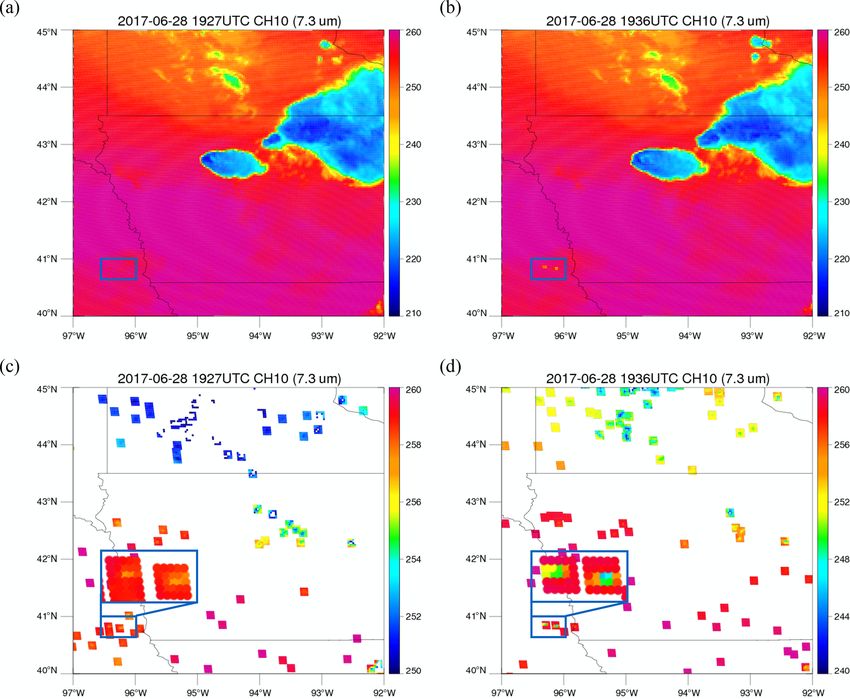
3756                                                                   Y. Lee et al.: Detection of convection using GOES-16

ing as accurately as possible, ground-based radars have been       formation, although this is largely limited to cloud top prop-
used during the short-term forecast. However, ground-based         erties. Convection detection algorithms using VIS and IR
radar data are not available over ocean or mountainous re-         sensors exist for both convective initiation (CI) and mature
gions. Therefore, this study explores whether high-temporal-       stages. With the recent growing interest in machine learn-
resolution data from recent operational geostationary satel-       ing techniques, many studies have applied machine learning
lite measurements from the Geostationary Operational En-           methods in detecting convection (Han et al., 2019; Zhang
vironmental Satellites (GOES) R Series can provide similar         et al., 2019; Cintineo et al., 2020), but knowledge in phys-
information to radar for the location of convection so that        ical features of convective clouds is still required to con-
it can be used for initializing forecast models over regions       struct a model that correctly learns during training. At the
without ground-based radar.                                        initial stages of convection, cloud tops grow vertically, and a
   Convection is classically defined from in-cloud vertical air    decrease in brightness temperature (Tb ) is observed accord-
motions (Steiner et al., 1995). However, since vertical veloc-     ingly. Many algorithms use decreased cloud top temperature
ity is rarely measured directly, the radar community initially     from the growth (related to the in-cloud vertical velocity) to
adopted radar reflectivity thresholds to define convection and     detect convective regions from various geostationary satel-
distinguish it from stratiform precipitation (Churchill and        lites over the globe such as GOES (Sieglaff et al., 2011;
Houze, 1984; Steiner et al., 1995). One problem with us-           Mecikalski and Bedka, 2006), Himawari-8 (Lee et al., 2017),
ing reflectivity threshold is its sensitivity to the selected      and Meteosat (Autonès and Claudon, 2019). Temporal trends
threshold for convection. If the threshold is set high, convec-    of Tb are evaluated on several channels around the water va-
tive regions where precipitation has just begun are not cap-       por absorption band or longwave infrared window band and
tured, while a threshold that is set too low will misclassify      combinations of these channels. Interest fields for CI include
some stratiform regions as convective. To address this issue,      temporal trend of Tb at 10.7 µm (or 11.2 µm) to infer cloud
Churchill and Houze (1984) separated precipitation types by        top cooling rates, (3.9–10.7 µm) to infer changes in cloud
using the horizontal structure of precipitation fields (Steiner    top microphysics, and (6.5–10.7 µm) to infer cloud height
et al., 1995). They classified a grid point as convective if the   changes relative to the tropopause (Mecikalski and Bedka,
grid point had rain rates twice as high as the average taken       2006). The main differences between the algorithms are the
over surrounding grid points or had reflectivity over 40 dBZ       tracking method of a cloud and the time period used to calcu-
(∼ 20 mm h−1 ). Steiner et al. (1995) refined this method with     late Tb change of the cloud. Clouds are usually tracked with
three criteria: intensity, peakedness, and surrounding area.       atmospheric motion vectors or a simple overlap method, and
They used the same threshold of 40 dBZ for intensity in            temporal trends of Tb are calculated over 15 min.
the first step, but grid points with reflectivity greater than        Convective clouds in their mature stage cannot be detected
the average reflectivity within a radius of 11 km as well          by the abovementioned algorithms as their cloud tops do not
as surrounding grid points are also classified as convective.      grow much in the vertical, and Tb decrease is not a major
Nonetheless, stratiform regions sometimes can have reflec-         feature that is applicable to such clouds. Overshooting top
tivity values greater than 40 dBZ. Zhang et al. (2008) used        (OT) is one of the clear indications of mature convective
two reflectivity criteria for convective precipitation – namely    clouds, and many existing algorithms used the OT feature
that the reflectivity be greater than 50 dBZ at any height and     in such clouds. There are two common approaches to detect-
greater than 30 dBZ at −10 ◦ C height or above. Zhang and          ing OTs: the brightness temperature difference method and
Qi (2010) define a grid point as convective if the vertically      the infrared window-texture method (Ai et al., 2017). The
integrated liquid water exceeds a threshold of 6.5 kg m−2 . Qi     brightness temperature difference method uses a difference
et al. (2013) developed a new algorithm that combined two          in Tb between the water vapor (WV) channel and IR win-
previous methods from Zhang et al. (2008) and Zhang and            dow channel (Tb,wv − Tb,IR ). Positive values of Tb,wv − Tb,IR
Qi (2010). By combining these two methods and modifying            due to the forcing of warm WV from below into the lower
the thresholds, they were able to decrease misclassification of    stratosphere are used as an indicator of OTs (Setvak et al.,
stratiform regions with strong bright band features, but could     2007). However, since the threshold for the difference be-
still miss some convective regions in their initial stage due to   tween two channels can depend on several factors, Bedka
a high-reflectivity threshold. The HRRR model uses a much          et al. (2010) suggested another method to detect OTs which
lower reflectivity threshold of 28 dBZ to detect convective        is called the infrared window-texture method. This method
regions and assigns a heating increment (Weygandt et al.,          takes advantage of a feature of OT in that it is an isolated
2016). While this is significantly lower than the thresholds       region with cold Tb surrounded by the relatively warm anvil
discussed above, its primary purpose is to initiate convection     region (Bedka et al., 2010). This method, unfortunately, can-
where there is significant echo present, while relying on the      not avoid having to choose Tb thresholds that vary accord-
model physics to assign the proper precipitation type.             ing to seasons or regions (Dworak et al., 2012). Bedka and
   While radars have been the preferred method for detecting       Khlopenkov (2016) tried to minimize the use of fixed detec-
convection, they are not the only instruments available. Vis-      tion criteria. They developed two OT detection algorithms
ible (VIS) and infrared (IR) radiances also contain some in-       based on IR and VIS channels, and an OT probability was

Atmos. Meas. Tech., 14, 3755–3771, 2021                                             https://doi.org/10.5194/amt-14-3755-2021
Y. Lee et al.: Detection of convection using GOES-16                                                                       3757

produced through a pattern-recognition scheme. The pattern        month statistical study to quantify the operational accuracy
that the scheme looks for is protrusion through the anvil         of the methods.
caused by strong updrafts. Another pattern that is obvious in
mature convective clouds with or without OT is a “lumpy sur-
face” from constant bubbling (Mecikalski and Bedka, 2006).        2     Data
Cloud top texture in VIS and IR channels has been explored
                                                                  2.1    The Geostationary Operational Environmental
using the Spinning Enhanced Visible and Infrared Imager
                                                                         Satellite R Series (GOES-R)
(SEVIRI) on the Meteosat-8 satellite in Zinner et al. (2008,
2013), respectively. In addition to evaluating spatial texture,   Earth-pointing instruments of GOES-R consist of the Ad-
Müller et al. (2019) explores spatiotemporal gradients of wa-     vanced Baseline Imager (ABI) with 16 channels, and the
ter vapor channels in SEVIRI to estimate updraft strength.        Geostationary Lightning Mapper (Schmit et al., 2017).
This study suggests a different way to calculate spatial gra-     GOES-16 is the first of the two GOES-R Series satellites
dients of visible channels in GOES-R to detect convection.        to provide data for severe weather forecast over the United
   The use of VIS and IR sensors in detecting convection          States and surrounding oceans (Schmit et al., 2017). Both Tb
can benefit significantly from the launch of National Oceanic     and reflectance data from the ABI were used to detect con-
and Atmospheric Administration’s (NOAA’s) GOES-R Se-              vective regions. Mesoscale data with 1 min temporal resolu-
ries which have high-resolution, rapidly updating (i.e., 1 min)   tion were used to fully exploit its high temporal resolution of
imagery. This study makes use of these new data, namely           the new instrument.
the 1 min data available from GOES-16 and GOES-17 in                 Reflectance at 0.64 µm (Channel 2) and Tb at 6.2 µm
“mesoscale sectors” to update methods for detecting con-          (Channel 8), 7.3 µm (Channel 10), and 11.2 µm (Channel 14)
vection in different stages. Mesoscale sectors are manually       were used in the study. Channel 2 is a “red” band with the
moved around to observe interesting weather events. One is        finest spatial resolution of 0.5 km. This fine spatial resolu-
developed for CI using Tb from an IR channel in GOES-R.           tion is useful to resolve lumpy or bubbling surfaces of clouds
As in previous papers measuring clout top cooling rate, tem-      in their mature stage. Channel 2 reflectance data were nor-
poral trends of the data were used, but since GOES-R has          malized by solar zenith angle so that a single threshold can
high temporal resolution, 10 consecutive data with 1 min in-      be used throughout the method regardless of locations of the
tervals were used. It has been challenging to correctly track     sun. Channel 14 is an IR longwave window band, which is a
convective clouds with 15 or 30 min interval data which have      good indicator of the cloud top temperature for cumulonim-
been used in previous studies due to the changing shape of        bus clouds (Müller et al., 2018). High reflectance and texture
convective clouds and merging or splitting of clouds. How-        of the cloud top seen in Channel 2 and cloud top height in-
ever, since clouds do not change as much within 1 min, using      ferred from Channel 14 are combined to determine locations
1 min data eliminates some of the errors from cloud move-         of mature convective clouds.
ments that needed to be dealt with in some previous studies,         Channels 8 and 10 are ABI water vapor channels with 2km
and the cooling rate is calculated applying linear regression     spatial resolution. Because Channel 8 sees WV at somewhat
on 1 min data over 10 min, rather than using Tb difference be-    higher altitudes than Channel 10, they can observe WV as-
tween 15 min. Another one is developed for mature convec-         sociated with updrafts as clouds develop upwards and were
tion using both reflectances from a VIS channel and Tb from       therefore used to detect early convection.
IR channels. For this algorithm, lumpy and rapidly chang-
ing surface and high cloud top height from mature convec-         2.2    NEXRAD and MRMS
tive clouds were used to detect clouds both with and without
OTs. Lumpiness is calculated using a Sobel operator which is      Multi-Radar/Multi-Sensor (MRMS) data developed at
an edge detection filter in image processing, and the lumpi-      NOAA’s National Severe Storms Laboratory were used for
ness is explored at each minute throughout 10 min to look         validation purposes. MRMS integrates the radar mosaic from
for regions with continuous bubbling. These two methods           the Next Generation Weather Radar (NEXRAD) with atmo-
were then combined to provide detection of convection in          spheric environmental data, satellite data, lightning, and rain
all stages. The above methods are not intended to replace         gauge observations to produce three-dimensional fields of
ground-based radars where these are available. Instead, the       precipitation (Zhang et al., 2016). These quantitative precipi-
focus here is complementing ground-based networks, either         tation estimation (QPE) products have a spatial resolution of
offshore or in other regions lacking coverage.                    1 km and temporal resolution of 2 min.
   The datasets that were used to detect convection and vali-        A “PrecipFlag” variable contained in the standard MRMS
date the results are described in Sect. 2, while the methods      product classifies precipitating pixels into seven categories:
used to identify initial and established convection are ex-       (1) warm stratiform rain, (2) cool stratiform rain, (3) con-
plained in Sect. 3. Section 4 highlights the results of each      vective rain, (4) tropical–stratiform rain mix, (5) tropical–
method. Two case studies were examined followed by a 1-           convective rain mix, (6) hail, and (7) snow. Details of the
                                                                  classification can be found in Zhang et al. (2016). It is a

https://doi.org/10.5194/amt-14-3755-2021                                           Atmos. Meas. Tech., 14, 3755–3771, 2021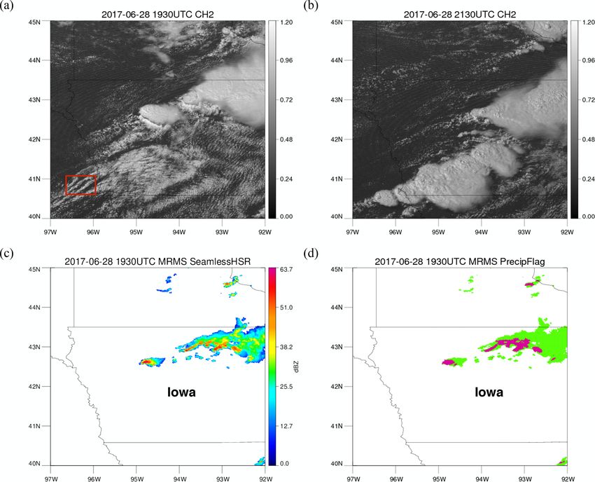
3758                                                                   Y. Lee et al.: Detection of convection using GOES-16

rather sophisticated classification of precipitation type as it
not only uses reflectivity at various heights, but also takes
into account vertically integrated liquid to distinguish con-
vective core from stratiform clouds (Qi et al., 2013). A re-
duced set of these classes was used to validate the convective
classification from GOES ABI data. In this study, warm strat-
iform rain, cool stratiform rain, and tropical–stratiform rain
mix are all assigned a stratiform rain type while grid points
with convective rain, tropical–convective rain mix, and hail
are assigned a convective rain type. Along with the classifica-
                                                                  Figure 1. (a) A typical shape of a convective cloud and its Tb dis-
tion product, MRMS provides a variable called “Radar QPE
                                                                  tribution around the convective core (blue line). (b) Schematic rep-
quality index (RQI)”. This product is associated with quality
                                                                  resentation of distributions of the upside down Gaussian matrix
of the radar data, which is a combination of errors coming        (green) and the Tb matrix (blue) when the cloud is convective.
from beam blockages and the beam spreading or ascending
with range (Zhang et al., 2016). This flag is used to mask
out regions with low radar data quality. Only data with RQI
greater than 0.5 are used in this study.                          observe small hydrometeors, but a Tb decrease at water va-
                                                                  por absorption bands of GOES-ABI is observed when these
                                                                  small hydrometeors start to develop. During the early con-
3     Methodology                                                 vective stages, Tb values that are sensitive to water vapor will
                                                                  decrease due to condensed cloud water droplets aloft gener-
This study examines methods to detect convective clouds at        ated by a strong updraft. Two ABI channels around the water
each life stage. Convective clouds can be divided into ac-        vapor absorption bands, Channel 8 (6.2 µm) and Channel 10
tively growing clouds and mature clouds. Actively growing         (7.3 µm), were selected to cover water vapor updrafts at dif-
clouds are usually clouds at the initial stage that grow nearly   ferent height levels. These channels were used to find small
vertically, while mature clouds are capped but continue to        regions consistent with developing clouds. If a cloud devel-
bubble due to the release of latent heat. They often move         ops continuously for 10 min and shows a large decrease in Tb
horizontally after they reach the tropopause. The proposed        over 10 min in either channel, the cloud is determined to be
method to detect actively growing cloud is similar to previ-      convective.
ous CI studies mentioned in the introduction in the sense that       To compute the Tb decrease in clouds, a window has
the method uses temporal trends of Tb . The high-temporal-        to be defined as it is usually difficult to precisely define
resolution data simplifies the method because the use of de-      the boundary of clouds, especially at the early stages of
rived wind motion in tracking clouds is no longer necessary.      convection. Since most of the early convective clouds are
One minute is short enough that cloud motion, at most, is to      smaller than 10 km in diameter, the window was defined as
the adjacent grid points, and clouds can be easily tracked by     a 10 km × 10 km box which is essentially a 5 × 5 matrix of
focusing on overlapped scenes.                                    satellite pixels consisting of 25 Tb values with 2 km resolu-
   The method to detect mature convective clouds is simi-         tion. Considering the fact that a convective core usually has
lar to previous studies by Bedka and Khlopenkov (2016) and        the lowest Tb within its neighborhood, the Tb matrix was
Bedka et al. (2019) in terms of using the texture of the cloud    formed around a pixel only if that pixel had the lowest Tb in
top surfaces to infer strong updrafts. Cloud top surfaces of      the 5 × 5 matrix. However, this criterion alone could not dis-
mature convective clouds are much bumpier than any other          tinguish convective cores from stratiform clouds and cloud
clouds, and their bumpiness is most evident in VIS images         edges which can also exhibit a local minimum. In addition
with the finest resolution. The following method uses a hor-      to the lowest Tb , the shape of convective clouds is therefore
izontal gradient of reflectance to represent the bumpiness of     also considered. As shown in the Fig. 1a, convective clouds
cloud tops, and the magnitude of the gradients is used to dis-    not only have the lowest Tb in their cores in all directions, but
tinguish convective cores from their anvil clouds. Cloud top      also have increasing Tb values away from the core, making
temperatures from Channel 14 are used to eliminate low cu-        their Tb distributions look like an inverted two-dimensional
mulus clouds that might appear bubbling.                          (2D) Gaussian distribution. To select Tb matrices that have
                                                                  this upside down Gaussian shape, an inverted 5 × 5 Gaus-
3.1    Detection of actively growing clouds with                  sian matrix that has mean and standard deviation of the Tb
       brightness temperature data                                matrix was created and compared with the Tb matrices. To
                                                                  focus the comparisons on the shape of the Tb distribution
In the early stage of convection, updrafts of water vapor         (Fig. 1b), the maximum Tb found in the 5 × 5 matrix was
eventually lead to condensation, the release of latent heat,      subtracted from all values, and Tb values were divided by the
and convective processes. Operational weather radars cannot       difference between maximum and minimum Tb to normalize

Atmos. Meas. Tech., 14, 3755–3771, 2021                                             https://doi.org/10.5194/amt-14-3755-2021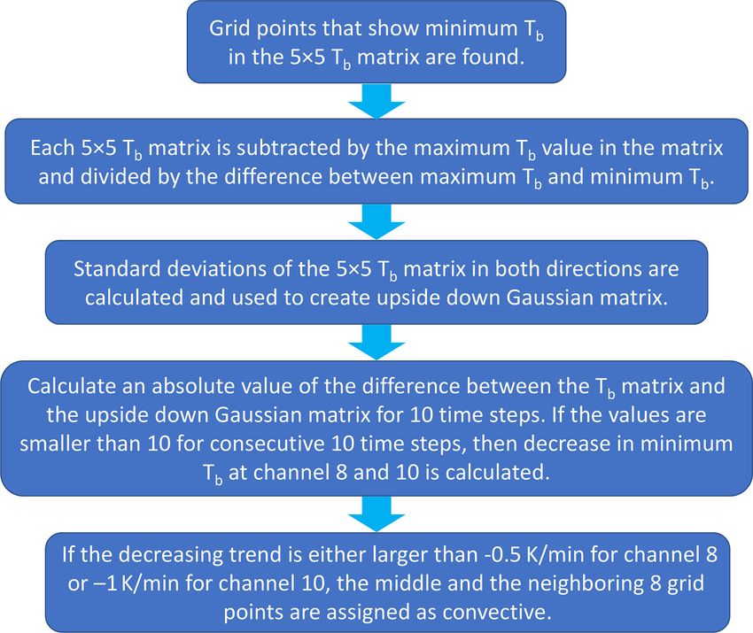
Y. Lee et al.: Detection of convection using GOES-16                                                                           3759

Figure 2. A flow chart to summarize the growing cloud detection method.

the Tb matrix itself. If the Tb matrix has a shape of a develop-     appropriate threshold that best represents the growth rate
ing cloud (i.e., 2D upside down Gaussian), the absolute value        for clouds in their early stages. These thresholds are cho-
of the difference between the Tb matrix and the upside down          sen based on the analysis of 1-month data during July of
Gaussian matrix will be small. A threshold of 10 for this ab-        2017. The 5 × 5 Tb windows that maintained the develop-
solute value of the difference between Tb matrix and upside          ing shape and had a decreasing trend of Tb during 10 min
down Gaussian matrix (sum of residuals between normal-               are collected over the 1-month period. A total of 38293 and
ized Tb and upside down Gaussian) was empirically deter-             97042 (for Channels 8 and 10, respectively) 5 × 5 windows
mined to exclude non-convective scenes. Tb matrices with             that show a decrease in Tb were collected, and precipitation
values greater than 10 are removed from the scene. This is           types from MRMS were assigned for each window. Future
done for all 10 consecutive Tb images that are 1 min apart.          MRMS convective flags up to 20 min after the detection pe-
Continuous overlaps of Tb matrices for 10 min imply that the         riod were included in the analysis because some time de-
cloud maintained a convective shape for 10 min, and there-           lays were observed in MRMS product when assigning con-
fore changes in Tb are calculated to assess if the cloud in          vective flags, especially for early convection. When compar-
the Tb matrices was growing. The minimum Tb values of                ing GOES products to future MRMS products, future loca-
the Tb matrices at each time step were linearly regressed            tions of GOES products were calculated assuming convec-
against time to measure a decreasing trend. If the fitted line       tion moves at the same speed at which clouds moved during
at each channel had a slope either smaller than −1 K min−1           the initial 10 min. Tables 1 and 2 show results applying differ-
for Channel 10 or −0.5 K min−1 for Channel 8, the grid point         ent thresholds ranging from −0.1 to −2.0 K min−1 . For each
with the lowest Tb at each time step for 10 min as well as the       row, 5 pixel × 5 pixel windows that show a larger tempera-
neighboring eight grid points in the window were classified          ture decrease than the corresponding threshold are collected,
as convective. This procedure is summarized in a flow chart          and they are analyzed for potential convection. Numbers in
in Fig. 2.                                                           the table represent the number of 5 × 5 windows that MRMS
   Water vapor channels have different sensitivity to water          precipitation flags were assigned to either non-convective or
vapor, and thus different values for the threshold are cho-          convective at the corresponding 10 min time window, as well
sen for each channel (Channels 8 and 10). Since growth               as pixels that were flagged as convective by MRMS in the
rate can vary depending on the surrounding environment               next 10 and 20 min to account for the fact that GOES can de-
and different evolution stages, it is important to find an           tect convection before the radar sees precipitation. However,

https://doi.org/10.5194/amt-14-3755-2021                                               Atmos. Meas. Tech., 14, 3755–3771, 2021
3760                                                                        Y. Lee et al.: Detection of convection using GOES-16

Table 1. Number of non-convective, convective, convective within 10 min, and convective within 20 min for using different threshold values
(Channel 8).

                 Threshold value    Non-convective     Convective      Convective       Convective     Overall accuracy
                 (K min−1 )                                          within 10 min    within 20 min          (%)
                 −0.1                          3634          2911              250               89          47.2
                 −0.2                           740          2264              154               40          76.8
                 −0.3                           277          1831              117               28          87.7
                 −0.4                           153          1504               87               21          91.3
                 −0.5                           104          1266               87               16          92.8
                 −0.6                            67          1051               44               10          94.3
                 −0.7                            49           851               30                7          94.8
                 −0.8                            32           691               27                5          95.8
                 −0.9                            22           576               21                4          96.5
                 −1.0                            12           477               19                3          97.7
                 −1.1                             7           396               16                3          98.3
                 −1.2                             5           321               14                2          98.5
                 −1.3                             4           267                9                1          98.6
                 −1.4                             3           222                9                0          98.7
                 −1.5                             2           180                8                0          98.9
                 −1.6                             1           134                7                0          99.3
                 −1.7                             1           105                7                0          99.1
                 −1.8                             1            89                6                0          99.0
                 −1.9                             1            74                4                0          98.7
                 −2.0                             1            54                2                0          98.2

Table 2. Number of non-convective, convective, convective within 10 min, and convective within 20 min for using different threshold values
(Channel 10).

                 Threshold value    Non-convective     Convective      Convective       Convective     Overall accuracy
                 (K min−1 )                                          within 10 min    within 20 min          (%)
                 −0.1                         21900          5041             1339              511          23.9
                 −0.2                          9225          3982              854              277          35.7
                 −0.3                          4357          3284              611              163          48.2
                 −0.4                          2241          2722              429              109          59.3
                 −0.5                          1234          2268              310               71          68.2
                 −0.6                           759          1954              233               40          74.6
                 −0.7                           479          1661              184               28          79.6
                 −0.8                           318          1430              139               22          83.3
                 −0.9                            22           576               21                4          86.1
                 −1.0                           147          1050               75               14          88.6
                 −1.1                           103           893               64               11          90.4
                 −1.2                            77           758               56               10          91.5
                 −1.3                            55           657               42                9          92.8
                 −1.4                            41           556               34                5          93.6
                 −1.5                            28           461               29                5          94.6
                 −1.6                            17           393               25                3          96.1
                 −1.7                            14           340               24                3          96.3
                 −1.8                            11           297               21                2          96.7
                 −1.9                             9           255               19                2          96.8
                 −2.0                             5           207               19                1          97.8

Atmos. Meas. Tech., 14, 3755–3771, 2021                                                  https://doi.org/10.5194/amt-14-3755-2021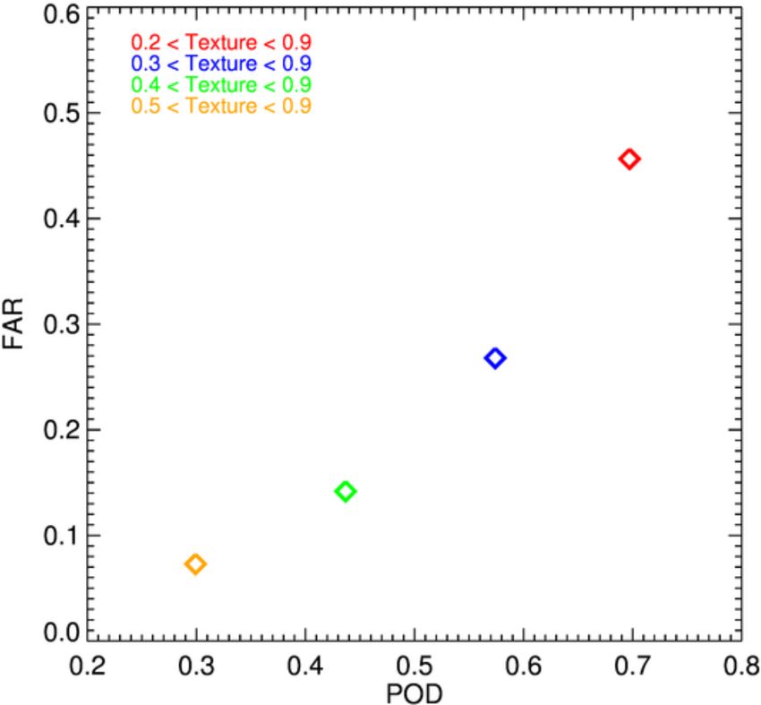
Y. Lee et al.: Detection of convection using GOES-16 3761
not all the detection by the method is done early since MRMS is highly correlated with the cloud optical depth (Minnis and
can also sometimes assign early convection as convective be- Heck, 2012) while Channel 14 brightness temperature is re-
fore it produces high reflectivity. The overall accuracy in the lated to cloud top temperature (Müller et al., 2018). These
last column is calculated by dividing the number of win- channels are used in GOES-R baseline product retrieval of
dows that were convective within 20 min (sum of convec- cloud optical depth and cloud top properties, respectively.
tive, convective within 10 min, and convective within 20 min) Any grid points with reflectance less than 0.8 or Tb greater
by the total number of the windows (sum of non-convective, than 250 K during 10 time steps (10 min) are removed since
convective, convective within 10 min, and convective within they generally represent thin or low clouds such as cirrus or
20 min). Some convective clouds in the early stage show growing clouds that can be identified by the CI method de-
a smaller decreasing trend than the thresholds, but using a scribed earlier. These thresholds are chosen rather generously
smaller value for the threshold can introduce clouds that do to include some convective clouds that have not grown into
not grow into deep convective clouds in the end. Clouds that deep convection yet, while still avoiding the misclassifica-
develop into deep convective clouds are eventually captured tion of low cumulus clouds and thin anvil clouds as convec-
by these thresholds in later times as they show rapid inten- tive. The threshold of 250 K is much warmer than typical val-
sification sooner or later. However, choosing a large cooling ues used in detecting deep convective features such as over-
rate for the threshold will lead to less detection of convec- shooting tops (Bedka et al., 2010) or enhanced V (Brunner
tive clouds as not a lot of windows show a large cooling rate. et al., 2007). A warmer threshold is intentionally chosen so
Therefore, thresholds of −0.5 and −1.0 K min−1 for Chan- that the method considers warmer convective clouds without
nels 8 and 10, respectively, are chosen so that reasonable those features in the next step when evaluating lumpiness of
amounts of convections are detected. The cooling rate ob- the cloud top. The choice of these thresholds is discussed in
served at Channel 8 is smaller than Channel 10 due to higher more detail in Sect. 4.3.
absorption at Channel 8. Channel 8 senses moisture at higher Once cold, highly reflective scenes are identified, regions
altitude, and thus when water vapor starts to condensate at with bubbling cloud top are found. Bubbling cloud top is
lower levels, it is less affected, and its Tb does not decrease a distinct feature that appears in convective clouds, even in
as much as in Channel 10. The matrix does not have to be their early stages. The lumpiness of cloud tops can be nu-
detected at both channels, but using two channels tends to merically represented by calculating horizontal gradients in
find the same vertically growing clouds over time by detect- the reflectance field with the Sobel–Feldman (Sobel) oper-
ing the cloud using Channel 8 first and then using Channel 10 ator which is commonly used in edge detection. The hori-
later. This method will be called the growing cloud detection zontal gradient is calculated at each pixel. The Sobel opera-
method hereinafter. tor convolves the target pixel and its surrounding eight grid
Furthermore, it is interesting to note that some clouds points with two kernels given in Eq. (1) to produce gradients
did not produce precipitation even with rapid growth over in the horizontal and vertical direction.
−2.0 K min−1 (for Channel 10). This would be due to mix-
+1 0 −1 +1 +2 +1
ing between convective cells and their dry environment or the
Gx = +2 0 −2 Gy = 0 0 0 (1)
highly non-linear nature of chances of precipitation.
+1 0 −1 −1 −2 −1
3.2 Detection of mature convective clouds with By using Eq. (2), gradients in each direction are combined
reflectance data to provide the absolute magnitude of the gradient at each
point.
Mature convective clouds consist of convective cores and q
stratiform or cirrus regions where clouds have detrained from Magnitude of gradient = G2x + G2y (2)
the core. The lack of discrete boundaries between differ-
ent types of clouds makes it difficult to separate convective
grid points from surrounding stratiform regions. Overshoot- Flat surfaces will have low gradients while cloud edges or
ing tops and enhanced-V pattern are well-known features in lumpy surfaces will have high gradients. This lumpy feature
mature convective clouds, but these do not appear until their is most evident in a VIS channel with the finest spatial reso-
strongest stage and not in all convective clouds. Using such lution of 0.5 km. IR fields are not very useful as the bright-
features associated with the deepest convective cores will ness temperature variations in these lumpy surfaces tend to
create a detection gap between early and mature stages of be quite small due to their relatively lower spatial resolution,
convection. The method described here tries to minimize the and only cloud edges stand out.
gap, while still accurately detecting convective clouds. The average of the horizontal gradients over the 10 1 min
Before evaluating the texture, only the grid points that are time steps is calculated for each grid point, and grid points
potentially parts of deep convection are selected using sim- are removed if the average was less than 0.4 or greater than
ple threshold values of VIS (ABI Channel 2; 0.65 µm) and IR 0.9. Values below 0.4 or above 0.9 generally imply either
(ABI Channel 14; 11.2 µm) channels. Channel 2 reflectance stratiform region with a flat surface or cloud edges with
https://doi.org/10.5194/amt-14-3755-2021 Atmos. Meas. Tech., 14, 3755–3771, 2021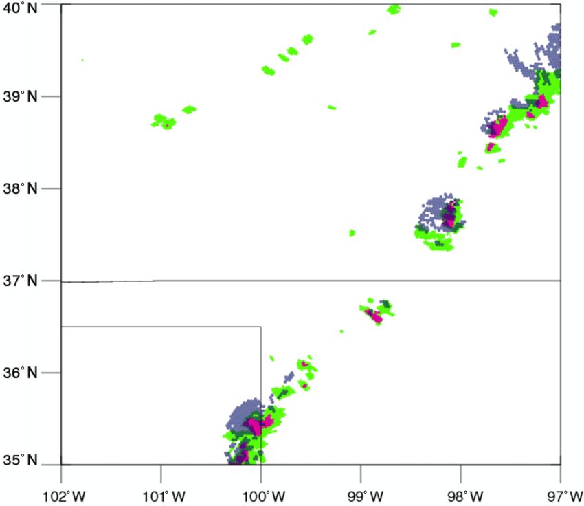
3762 Y. Lee et al.: Detection of convection using GOES-16
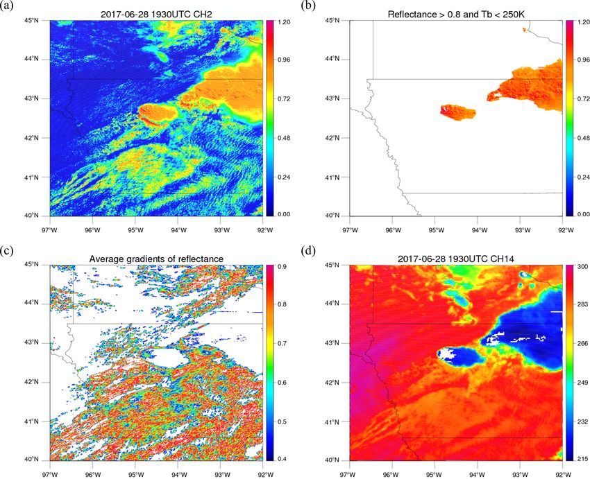
Figure 3. (a) GOES-ABI 0.65 µm visible channel imagery (0.5 km) at 19:30 UTC on 28 June 2017 over Iowa. Numbers on the color bar rep-
resent reflectances. The red box indicates regions where two convective cells are detected by the growing cloud detection method. (b) GOES-
ABI 0.65 µm visible channel imagery at 21:30 UTC on 28 June 2017. (c) MRMS Seamless Hybrid Scan Reflectivity (SHSR) at 19:30 UTC
on 28 June 2017. (d) MRMS PrecipFlag at 19:30 UTC 28 June 2017. Pink represents convective while green represents stratiform.
very high gradients, respectively. The thresholds are chosen 4 Results and discussion
to produce relatively low false alarms comparing results us-
ing other thresholds. Results using other thresholds are also 4.1 28 June 2017
shown in Sect. 4.3 for a comparison. The remaining grid
points were then interpolated into 1 km maps to be consistent Supercell thunderstorms developed in Iowa and produced
with the spatial resolution of the MRMS dataset. Neighbor- several tornado touchdowns. In Fig. 3a, deep convection
ing grid points were grouped to form clusters, and only the had already developed over central Iowa at 19:30 UTC, and
clusters with more than five grid points were assigned as a two convective cells in the red box started to develop in
mature convective cloud to remove noise. This method will southwest Iowa, although they do not stand out from sur-
be called the mature cloud detection method hereinafter. rounding low clouds in the VIS image. These two convec-
tive clouds became parts of major storm system that formed
around 21:30 UTC, producing the tornadoes (Fig. 3b) in the
area. MRMS Seamless Hybrid Scan Reflectivity (SHSR),
which gives reflectivity at the lowest possible vertical level,
is shown in Fig. 3c, and the MRMS PrecipFlag product is
Atmos. Meas. Tech., 14, 3755–3771, 2021 https://doi.org/10.5194/amt-14-3755-2021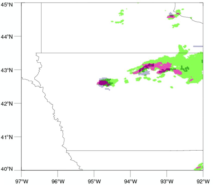
Y. Lee et al.: Detection of convection using GOES-16                                                                             3763

Figure 4. (a) GOES-ABI 7.3 µm infrared channel imagery (K) at 19:27 UTC on 28 June 2017. Blue box denotes regions where two convective
clouds start to grow. (b) Same as (a), but at 19:36 UTC. (c) Tb matrices obtained from Channel 10 (7.3 µm) that have the Gaussian shape
at 19:27 UTC on 28 June 2017. Blue box denotes the same region as the blue box in (a). Note that the scale of the color bar is adjusted
from (a, b) to better observe convective initiation. (d) Same as (c), but at 19:36 UTC.

shown in Fig. 3d. Convection is colored in pink and strati-           developing cells (Gaussian shape) at 19:27 and 19:36 UTC.
form in green. Although deep convections over the central             However, not all of the matrices in these figures showed the
and northeast part of Iowa were assigned as convective in             evolution of the developing cells (decreasing minimum Tb
MRMS at 19:30 UTC, the two growing clouds in the red                  over 10 K) between the two time steps. The two matrices in
box in Fig. 3a were not assigned a convective flag until              the blue box satisfied both criteria of maintaining the shape
19:48 UTC.                                                            of developing cells and growing vertically over 10 time steps
   Figure 4a shows brightness temperatures for ABI Chan-              while other matrices did not satisfy either one of the criteria.
nel 10 (7.3 µm) at 19:27 UTC. The two growing convective              These two matrices contain early convective clouds that grow
cells in the blue box are shown in barely visible yellow sur-         into deep convection shown in Fig. 3b, and they are correctly
rounded by high Tb values. The one on the left was detected           captured by this method.
using 10 min data from 19:25 UTC, but since both clouds                  Results for the detection of mature convective clouds are
were detected together starting at 19:27 UTC, a scene from            shown in a step-by-step fashion in Fig. 5. Figure 5a is the
19:27 UTC was used to demonstrate the method. Figure 4c               same as in Fig. 3a but is mapped using a different color ta-
and d show Tb matrices that exhibited the correct shape for           ble for better comparisons between steps. Figure 5b shows

https://doi.org/10.5194/amt-14-3755-2021                                                Atmos. Meas. Tech., 14, 3755–3771, 2021
3764                                                                           Y. Lee et al.: Detection of convection using GOES-16

Figure 5. (a) Same as Fig. 3a, but using different color table. (b) From the reflectance map in (a), regions that have reflectances over 10 min
less than 0.8 or have Tb values greater than 250 K over 10 min are assigned reflectance of zero, and therefore colored in white. (c) Map of
average gradients of reflectances over 10 min. Regions with average gradient less than 0.4 or greater than 0.9 are colored in white. (d) GOES-
ABI 11.2 µm infrared channel imagery (K) at 19:30 UTC on 28 June 2017. Regions that passed two criteria from (b) and (c) are colored in
white.

the pixels retained after eliminating all the grid points that            ing in Fig. 5d. Using a reflectance threshold sometimes lim-
did not meet the reflectance and Tb thresholds (minimum re-               its the detection of shaded convective regions that exhibits
flectance over 10 time steps greater than 0.8 and maximum                 lower reflectance than the threshold of 0.8. This is the case
Tb over 10 time steps less than 250 K). Figure 5c shows the               for the small imbedded white regions in the midst of high-
horizontal gradient values after applying the Sobel opera-                reflectance regions shown in Fig. 5b. However, these regions
tor. The color bar is set to be within the range of 0.4 and               are relatively small, and once they are upsampled into 2 km
0.9 to display potential convective regions that passed these             maps through nearest-neighbor interpolation, some of these
thresholds in colors. White regions are either regions that               regions are included in the detection as shown in Fig. 5d.
have average gradients greater than 0.9 such as cloud edges                  Detection from GOES and MRMS is compared in
or thin cirrus clouds, or regions that have average gradients             MRMS’s resolution of 1 km, and in such high resolution,
less than 0.4 such as clear sky or stratiform regions. Even-              the location of a cloud seen from GOES and MRMS can
tually, only the regions that meet the criteria in both Fig. 5b           be slightly different due to parallax displacement. For a bet-
and c are assigned to convection and shown as white shad-                 ter comparison between detection from GOES and MRMS,

Atmos. Meas. Tech., 14, 3755–3771, 2021                                                      https://doi.org/10.5194/amt-14-3755-2021
Y. Lee et al.: Detection of convection using GOES-16 3765
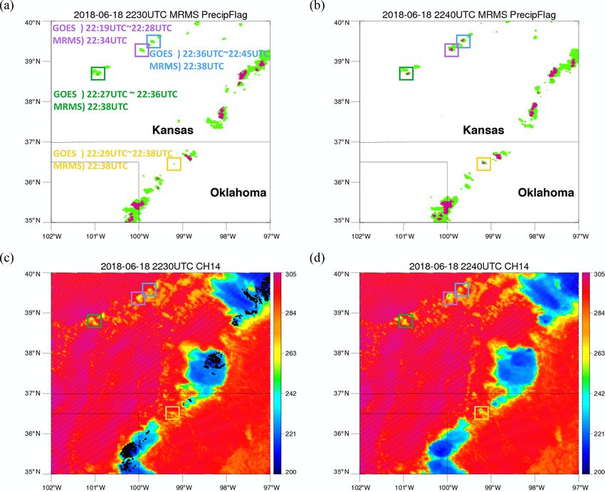
22:40 UTC is shown in Fig. 7a and b, respectively. The green
color represents stratiform and the pink color represents con-
vective clouds. Figure 7c and d are Tb maps of the same scene
at 22:30 and 22:40 UTC, respectively. Growing clouds shown
in purple, blue, yellow, and green boxes are detected by the
growing cloud detection method, but all starting from differ-
ent time. Times that each cloud is detected by GOES and
MRMS are shown in Fig. 7a. Time for the growing cloud
detection method is a period as the method uses 10 consec-
utive 1 min data. Convection in the purple box was detected
6 min earlier than MRMS detection considering the last data
used in the growing cloud detection method at 22:28 UTC.
Similarly, a cloud in the green box was detected a little ear-
lier by GOES than MRMS. The growing cloud in the yellow
box was detected at the same time by GOES and MRMS. On
the other hand, the growing cloud in the blue box was de-
tected later than MRMS detection at 22:38 UTC. This cloud
did not grow rapidly enough during 22:30–22:40 UTC pe-
Figure 6. Convective regions detected by GOES-16 (white regions riod as shown in Tb maps of Fig. 7c and d and did not meet
in Fig. 5d) are colored in navy on top of MRMS PrecipFlag at the Tb threshold for Channel 10 at the onset of convection.
19:30 UTC on 28 June 2017. (Same figure as Fig. 3d. Pink rep- However, it was detected by Channel 8 as it grew higher alti-
resents convective while green represents stratiform.) tudes. This shows that a cloud that initially did not show high
growth rate can have high growth rate as it vertically grows
and can be detected by Channel 8 later in time. These results
parallax correction based on Vicente et al. (2002) is ap- show that even though the thresholds for the growing cloud
plied to GOES detection using a constant cloud top height detection method can miss some convective clouds that grow
of 10 km. Convective regions detected by GOES (Fig. 5d) slowly in the beginning, the thresholds were adequate for de-
are plotted with the parallax correction on top of the MRMS tecting rapidly growing convective storms which are of more
map (Fig. 3d), and it is shown in Fig. 6. When compared to interest during the forecast.
high-reflectivity regions in Fig. 3c and convective regions in Black regions superimposed on the brightness tempera-
Fig. 3d, convective regions, while not perfectly aligned due ture map in Fig. 7c represent convective regions identified by
to a number of dynamic geometric reasons, do have a high the mature convection method, and Fig. 8 shows a figure of
degree of correspondence between the two detection meth- the black regions overlaid on top of the MRMS PrecipFlag
ods. However, a straight line around 43.7◦ N at the right edge map (Fig. 7a). There are slight misalignments of detected
of Fig. 5d is definitely not a convective region, and it is due convective clouds between MRMS PrecipFlag products and
to unrealistically high reflectance in the raw satellite dataset. GOES results possibly due to sheared vertical structures of
These kinds of artifacts were removed later in Sect. 4.3 when the storms. One other thing to note here is that the convec-
the method was applied to a full month of data. However, tive area detected by the mature cloud detection method is
multiple lines are difficult to remove at this stage in the pro- greater than what is detected in the previous case. This could
cessing and will result in false alarm. As quality control pro- be due to the dependency of lumpiness on some geometrical
cedures on ABI are improved, this may no longer be a source considerations. Lumpiness is a function of the pixel spatial
of significant errors. resolution, differences in optical depth, and shadows. Spa-
tial resolution decreases away from the Equator, but higher
4.2 18 June 2018 solar zenith angles (due to altitude or time of day) not only
increases optical depth, they also increase shadows. While
Another case was examined to evaluate the methods under this can of course be dealt with, it was ignored in this study
different conditions. Severe storms developed over the Great which serves primarily as a proof of concept, as the method
Plains in 18 June 2018, producing hail on the ground. At generally finds the convective core correctly.
22:30 UTC, sporadic storms across Kansas and Oklahoma
were observed by GOES-16. This scene contains both grow- 4.3 Statistical results with 1-month data
ing and mature convective clouds that are detected by MRMS
during the 22:30–22:40 UTC period. In particular, four ver- Pixel-based validation of the two methods is conducted us-
tically growing clouds in this scene show different evolution ing 1 month of data measured during June 2017. Results are
and thus allow more elaboration on the growing cloud detec- validated against MRMS data as ground-based radar is used
tion method. MRMS PrecipFlag for the scene at 22:30 and to detect convective regions during the short-term forecast,
https://doi.org/10.5194/amt-14-3755-2021 Atmos. Meas. Tech., 14, 3755–3771, 20213766 Y. Lee et al.: Detection of convection using GOES-16
Figure 7. (a) MRMS PrecipFlag at 22:30 UTC on 18 June 2018. Pink represents convective while green represents stratiform. Times next
to each box represent the times of GOES data used in the growing cloud detection method and time of detection by MRMS. (b) MRMS
PrecipFlag at 22:40 UTC on 18 June 2018. (c) GOES-ABI 11.2 µm infrared channel imagery (K) at 22:30 UTC on 18 June 2018 over the
Great Plains. (d) Same as (c), but at 22:40 UTC.
and precipitation is a rather direct indicator of convection as convective. GOES-C/MRMS-NC denotes a “false alarm”
in all stages. Since MRMS detection comprises convection that GOES detected as convective, but MRMS did not.
in all stages, MRMS data are compared with GOES detec- Lastly, GOES-NC/MRMS-NC denotes a “correct negative
tion combining the two methods. Table 3 is a contingency case” that neither MRMS nor GOES detected as convective.
table applying both methods to 1-month data and comparing From the contingency table, verification metrics of probabil-
in MRMS’s grids with a spatial resolution of 1 km. C repre- ity of detection (POD) and false alarm rate (FAR) can be
sents convection detected by either GOES or MRMS, and calculated as below.
NC represents non-convective regions. GOES-C/MRMS-C hits false alarm
is “hits” that both MRMS and GOES methods detected as POD = FAR = (3)
hits + misses hits + false alarm
convective within 5 km. In the case of the growing cloud de-
tection method, on the other hand, hits are defined if MRMS POD and FAR are useful tools in evaluating detection skill
assigned convective within 30 min due to earlier detection of a binary problem. POD and FAR calculated from Table 3
by this method. GOES-NC/MRMS-C denotes “misses” that are 45.3 % and 14.4 %. Since POD and FAR can vary de-
GOES missed detecting convection while MRMS assigned pending on the thresholds used in each method, choosing dif-
ferent thresholds is examined further.
Atmos. Meas. Tech., 14, 3755–3771, 2021 https://doi.org/10.5194/amt-14-3755-2021Y. Lee et al.: Detection of convection using GOES-16 3767
Figure 8. Convective regions detected by GOES-16 (in Fig. 7c) Figure 9. Plot of probability of detection (POD) and false alarm
are colored in navy on top of MRMS PrecipFlag at 22:30 UTC on ratio (FAR) using different texture thresholds of the mature cloud
18 June 2018 (Fig. 7a). Pink represents convective while green rep- detection method. The Tb and reflectance thresholds are kept con-
resents stratiform). stant with 250 K and 0.8, respectively.
Table 3. Contingency table of results applying both of GOES de-
tection methods and validating against MRMS data during June different combinations of the three thresholds (reflectance
of 2017. Pixel-based validation is conducted to produce this at Channel 2 and Tb at Channel 14 to remove shallow and
table. C and NC represent convective and non-convective, re- low clouds, and horizontal gradients of reflectance at Chan-
spectively. GOES-C/MRMS-C denotes “hits” that both MRMS nel 2 to remove cloud edges as well as clouds with flat
and GOES methods detected as convective within 5 km. GOES- cloud top surfaces) are presented to show how they differ
NC/MRMS-C denotes “misses” that GOES missed detecting con- from the chosen thresholds. Two thresholds for cloud top tex-
vection while MRMS assigned as convective. GOES-C/MRMS-NC ture, which are essentially horizontal gradients of reflectance,
denotes “false alarm” that GOES detected as convective, but MRMS
are evaluated first. The upper threshold does not change re-
did not. GOES-NC/MRMS-NC denotes a “correct negative case”
that neither MRMS nor GOES detected as convective. Percentages
sults much (not shown), and cloud edges are effectively re-
in the parenthesis are obtained by dividing each number by the total moved by the threshold of 0.9. The lower bound of the texture
number. thresholds are varied, keeping the upper threshold and the
Tb and reflectance thresholds constant. Resulting FAR and
MRMS-C MRMS-NC POD are shown in Fig. 9. Using 0.5 (yellow) misses signifi-
cant amounts of convective regions while using lower values
GOES-C 1 759 878 (2.73 %) 297 291 (0.46 %)
(blue and red) substantially misclassifies stratiform regions
GOES-NC 2 125 739 (3.30 %) 60 244 716 (93.51 %)
with flat cloud tops as convective, although their PODs are
much higher. Using 0.2 gives the closest results from the
pixel-based validation in Zinner et al. 2013 using lightning
Most of the detection is from the mature cloud detec- data. However, FAR of 45.6 % when using 0.2 is no differ-
tion method as mature convective clouds account for a much ent from a random chance of 50 % that it is no longer useful,
larger area. The mature cloud detection method alone has while POD of 29.9 % when using 0.5 will not give much in-
FAR of 14.2 % and POD of 43.7 %. FAR and POD of the formation. Therefore, values of 0.4 and 0.9 (green diamond
growing cloud detection method including 30 min data are in Fig. 9) were chosen as a reasonable compromise between
22.2 % and 3.9 %, respectively. Relatively small FAR com- POD and FAR.
pared to FAR from Tables 1 and 2 (1 − overall accuracy val- POD and FAR using different combinations of Tb and re-
ues) would be because Tables 1 and 2 are obtained based flectance thresholds are plotted in Fig. 10, and this time tex-
on each cloud while FAR and POD are calculated based on ture thresholds are kept constant with 0.4 and 0.9. The Tb
each grid point. Two PODs from the two methods (43.7 % threshold is varied from 230 to 250 K, and the reflectance
and 3.9 %) do not add up to 45.3 % (POD calculated from threshold is varied from 0.7 to 0.9. There is a trade-off be-
Table 3) due to overlapped detection. Since the mature cloud tween detecting more convective clouds that are transition-
detection method resort to several thresholds, results using ing into a mature stage and incorrectly assigning cumulus
https://doi.org/10.5194/amt-14-3755-2021 Atmos. Meas. Tech., 14, 3755–3771, 20213768 Y. Lee et al.: Detection of convection using GOES-16
and stratiform classification scheme improves QPE retrieval
(Qi et al., 2013; Petković et al., 2019).
As shown from these results, there are no perfect thresh-
olds that can separate convective and stratiform clouds. Nev-
ertheless, threshold values were chosen in line with our main
objective – to avoid high FAR as much as possible and have
decent POD comparable to radar products. Avoiding FAR is
a higher priority than reaching higher POD as giving false in-
formation is most detrimental during data assimilation. Low
FAR of 14.4 % is achieved, and among those misclassified
pixels, 96.4 % of them are at least raining. Since the main
objective of data assimilation is to have good initialization
of precipitation, applying these methods during data assim-
ilation can still be beneficial in case the forecast model did
not produce precipitation. Unfortunately, significant amounts
of convective areas assigned by the radar product are missed.
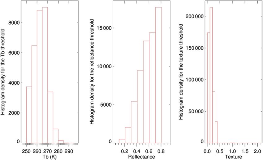
As shown in Fig. 11, most of the missed regions are excluded
due to the flat surface, and this is an intrinsic problem of us-
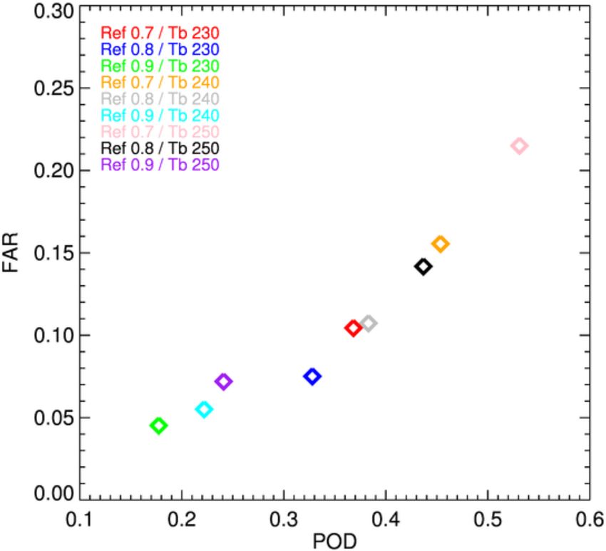
Figure 10. Plot of probability of detection (POD) and false alarm ing VIS and IR bands. If a convective cloud is developing in
ratio (FAR) for different combinations of Tb and reflectance thresh- a less cloudy scene, it can be detected by the method most of
olds. The texture threshold of 0.4 and 0.9 are kept constant.
the time. However, in case of a hurricane where cloud tops
are rather flat, or multi-layer clouds where cloud top informa-
tion is decoupled from what is underneath, convection will be
clouds as convective clouds. Having lower values for the Tb missed by the detection method. Furthermore, flat cloud top
threshold or higher value for the reflectance threshold leads regions close to bubbling area might still be convective by
to small FAR, but also leads to small POD. To make this MRMS due to high reflectivity, leading those regions to be
method effective and reduce FAR as much as possible for its classified as missed. The thresholds can be adjusted for other
potential use in the short-term forecast, 250 K for the Tb and applications that may require higher POD.
0.8 for the reflectance threshold (black diamond in Fig. 10a)
are chosen. In data assimilation, it is preferable to provide no
constraints than to provide the model with the incorrect lo-
cation of convection. A value of 240 K and 0.7 (orange) also 5 Conclusion and summary
showed similar results, but 250 K and 0.8 were chosen due to
lower FAR. This study explores two methods to detect convective clouds
Despite its FAR being relatively small, the method misses in two different stages using GOES-R ABI data with 1 min
significant amounts of convective areas observed by MRMS. intervals. Using such high-temporal-resolution data facili-
Therefore, regions that were missed are evaluated further tates cloud tracking in a more effective way and helps re-
to investigate which threshold contributed most to missing duce uncertainties coming from cloud tracking when calcu-
those regions. Figure 11 shows histograms of Tb , reflectance, lating decreases in Tb of the same cloud. Convective clouds
and texture in the convective regions that were missed by the in the early stage were detected using Tb values of ABI chan-
above method. It is clear from the figure that the largest num- nels 8 and 10. These channels were used to find cloud scenes
ber of misses were due to low texture values (87.6 % of all with the developing shape of convective clouds. They were
missed regions has lower gradients than 0.4). There are many then used again to calculate the Tb decrease for those which
reasons why convective regions appear to have flat cloud top maintained the developing shape for 10 min. A cloud scene
surfaces. Anvil or thick cirrus clouds above convective re- that had a consistent developing shape and a large decrease in
gions can smooth out or cover bubbling cloud tops, and there Tb over 10 min was classified as convective by this method.
is simply no way to avoid this problem. Another reason may Mature convective clouds were detected by masking out re-
be the nature of the classification method. Since classifica- gions with high Tb in ABI Channel 14 and low reflectance
tion by MRMS is determined by rain rate, even if convective in ABI Channel 2 and finding regions with high horizontal
clouds are in a decaying mode and do not bubble anymore, gradients of reflectance over the course of 10 min. Results
clouds can still continue to precipitate considerable amounts, from this mature cloud detection method were mostly con-
which would lead to convective category in the MRMS prod- sistent with the radar-derived products, although this method
uct. It is also possible that it is due to a misclassification of is limited to daytime use only. Nevertheless, it detects a wide
trailing stratiform regions using radars. There is indeed ongo- range of convective area, not just regions with overshooting
ing research in the radar community since a better convective tops. Both methods are provided as a testing concept with
Atmos. Meas. Tech., 14, 3755–3771, 2021 https://doi.org/10.5194/amt-14-3755-2021Y. Lee et al.: Detection of convection using GOES-16 3769
Figure 11. Histograms of Tb , reflectance, and texture values if a pixel was assigned to be convective by MRMS, but not detected by the
mature cloud detection method due to each of the thresholds.
several thresholds, and these thresholds can be tuned for an Author contributions. All three authors designed the experiments.
operational use if needed. YL processed and analyzed the data. CDK and MZ gave feedbacks
These methods work well for well-structured convective with their insights at every step of the data analysis. The paper was
clouds, but there are limitations to this method, as with most written jointly by YL, CDK, and MZ.
algorithms using IR and VIS sensors. Cirrus cloud shields are
the biggest problem as they block Tb decreases underneath
and smooth out lumpy reflectance surfaces. However, these Competing interests. The authors declare that they have no conflict
of interest.
methods can still be useful for defining convection for as-
similation into models where radar data are not available. Be-
cause regions identified as convective are most likely convec-
Financial support. This research is supported by CIRA’s Graduate
tive (∼ 85 % accuracy; 100 % − (FAR of 14.4 %)), this can
Student Support Program, as well as the WMO sponsored ICEPOP-
easily be assimilated while setting cloudy regions to “miss- 18 project through the Korean Meteorological Administration.
ing” since the accuracy of detecting convection under large
cirrus shields is poor. Furthermore, results using a Sobel op-
erator, which is commonly used in image processing, implies Review statement. This paper was edited by Bernhard Mayer and
that applying machine learning can be beneficial if the model reviewed by two anonymous referees.
can be set up to learn lumpy texture of convective clouds dur-
ing training.
References
Data availability. NEXRAD reflectivity data were obtained Ai, Y., Li, J., Shi, W., Schmit, T. J., Cao, C., and Li, W.: Deep con-
by NOAA’s National Centers for Environmental Information: vective cloud characterizations from both broadband imager and
https://doi.org/10.7289/V5W9574V (NOAA National Weather hyperspectral infrared sounder measurements, J. Geophys. Res.,
Service (NWS) Radar Operations Center, 1991). Past MRMS 112, 1700–1712, https://doi.org/10.1002/2016JD025408, 2017.
datasets are available at http://mtarchive.geol.iastate.edu/ (last Autonès, F. and Claudon, M.: Algorithm Theoretical Basis Docu-
access: 2 May 2021, IEM Mtarchive, 2021). GOES-R data were ment for the Convection Product Processors of the NWC/GEO,
made available by the Cooperative Institute for Research in the available at : https://www.nwcsaf.org/ (last access: 2 May 2021),
Atmosphere (CIRA). 2019.
Bauer, P., Thorpe, A., and Brunet, G.: The quiet revolu-
tion of numerical weather prediction, Nature, 525, 47–55,
https://doi.org/10.1038/nature14956, 2015.
https://doi.org/10.5194/amt-14-3755-2021 Atmos. Meas. Tech., 14, 3755–3771, 2021You can also read