Surges of Harald Moltke Brae, north-western Greenland: seasonal modulation and initiation at the terminus - The ...
←
→
Page content transcription
If your browser does not render page correctly, please read the page content below
The Cryosphere, 15, 3355–3375, 2021
https://doi.org/10.5194/tc-15-3355-2021
© Author(s) 2021. This work is distributed under
the Creative Commons Attribution 4.0 License.

Surges of Harald Moltke Bræ, north-western Greenland: seasonal
modulation and initiation at the terminus
Lukas Müller1,2 , Martin Horwath1 , Mirko Scheinert1 , Christoph Mayer3 , Benjamin Ebermann1 , Dana Floricioiu4 ,
Lukas Krieger4 , Ralf Rosenau1 , and Saurabh Vijay5,6
1 Technische Universität Dresden, Institut für Planetare Geodäsie, Dresden, Germany
2 Institute
          of Geodesy and Photogrammetry, ETH Zurich, Zurich, Switzerland
3 Bavarian Academy of Sciences and Humanities, Munich, Germany
4 German Aerospace Center, Wessling, Germany
5 DTU Space – National Space Institute, Kongens Lyngby, Denmark
6 Byrd Polar & Climate Research Center, Columbus, USA

Correspondence: Lukas Müller (lukamueller@ethz.ch)

Received: 5 September 2020 – Discussion started: 6 November 2020
Revised: 22 May 2021 – Accepted: 27 May 2021 – Published: 21 July 2021

Abstract. Harald Moltke Bræ, a marine-terminating glacier          through seasonally changing meltwater availability. Thus, the
in north-western Greenland, shows episodic surges. A recent        seasonal amplitude remains high for 2 or more years until the
surge from 2013 to 2019 lasted significantly longer (6 years)      fast ice flow has flattened the ice surface and the glacier sta-
than previously observed surges (2–4 years) and exhibits a         bilizes again.
pronounced seasonality with flow velocities varying by 1 or-
der of magnitude (between about 0.5 and 10 m d−1 ) in the
course of a year. During this 6-year period, the seasonal ve-
locity always peaked in the early melt season and decreased        1   Introduction
abruptly when meltwater runoff was maximum. Our data
suggest that the seasonality has been similar during previous      Surge-type glaciers are characterized by an alternation of
surges. Furthermore, the analysis of satellite images and dig-     long periods of low flow velocity (several to hundreds of
ital elevation models shows that the surge from 2013 to 2019       years, quiescent phases) and comparably short periods with
was preceded by a rapid frontal retreat and a pronounced           velocities increased by at least 1 order of magnitude (1–
thinning at the glacier front (30 m within 3 years).               15 years, active phases or surge events) (Jiskoot, 2011; Benn
    We discuss possible causal mechanisms of the seasonally        and Evans, 1998; Bhambri et al., 2017). These rapid changes
modulated surge behaviour by examining various system-             in ice flow are triggered by internal instabilities and are
inherent factors (e.g. glacier geometry) and external factors      mostly independent of external influences like weather or cli-
(e.g. surface mass balance). The seasonality may be caused         mate (Jiskoot, 2011; Benn et al., 2019). Therefore, knowl-
by a transition of an inefficient subglacial system to an ef-      edge about the occurrence and distribution of surge-type
ficient one, as known for many glaciers in Greenland. The          glaciers and an understanding of the underlying surge mech-
patterns of flow velocity and ice thickness variations indi-       anisms are crucial when studying the relationship between
cate that the surges are initiated at the terminus and de-         climate change and changes in glacier dynamics.
velop through an up-glacier propagation of ice flow accelera-         Only about 1 % of the glaciers worldwide are assumed to
tion. Possibly, this is facilitated by a simultaneous up-glacier   be surge type (Jiskoot, 1999). Surge-type glaciers normally
spreading of surface crevasses and weakening of subglacial         cluster in certain regions (such as Alaska, Svalbard and the
till. Once a large part of the ablation zone has accelerated,      Karakoram) where the conditions are favourable for surge
conditions may favour substantial seasonal flow acceleration       behaviour (e.g. a soft glacier bed and an at least partially
                                                                   temperate regime) (Sevestre and Benn, 2015; Jiskoot, 2011).

Published by Copernicus Publications on behalf of the European Geosciences Union.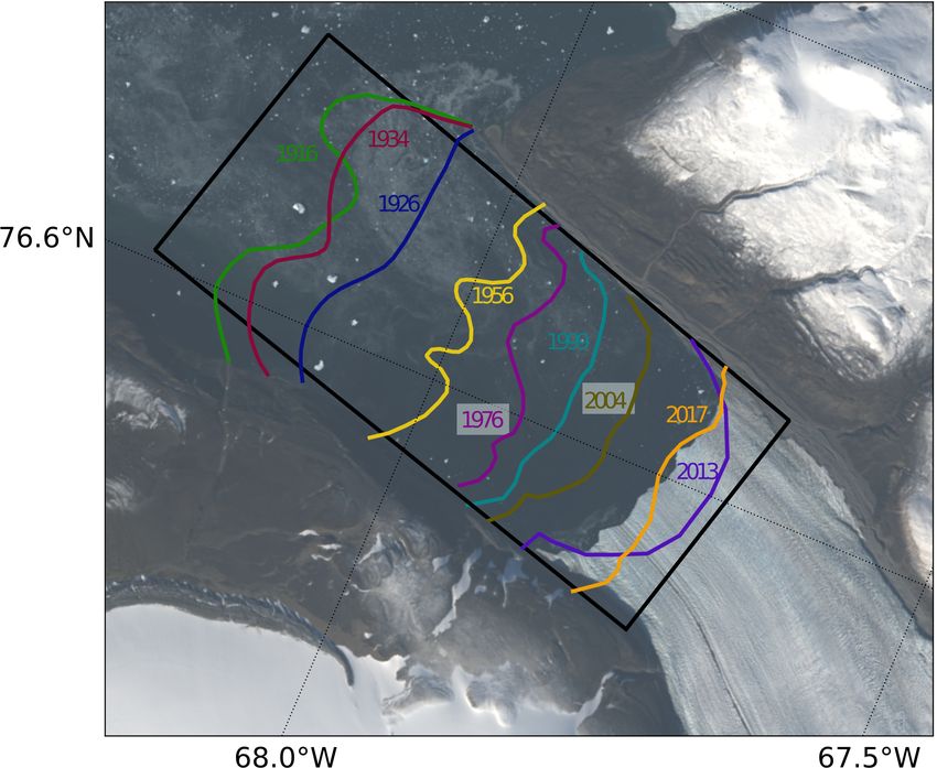
3356                                                                         L. Müller et al.: Surges of Harald Moltke Bræ

Some surge-type glaciers are also known in Greenland. For            Two different mechanisms, both involving an internal in-
example, clusters of surge-type glaciers in central–western       stability, have been considered as possible causes of glacier
Greenland and central–eastern Greenland were reported by          surges: (A) thermal and (B) hydrological (Murray et al.,
Sevestre and Benn (2015). Apart from these clusters, Hagen        2003). Mechanism (A) occurs in glaciers which are partly
Bræ in north-eastern Greenland is assumed to be a surge-type      frozen to the glacier bed such that the ice flow is in part
glacier (Solgaard et al., 2020).                                  restricted during the quiescent phase. The increasing shear
   Another surge-type glacier isolated from the known surge       stress due to the steepening of the reservoir area during the
clusters is Harald Moltke Bræ, a marine-terminating glacier       quiescent phase can subsequently trigger a feedback with an
in north-western Greenland. Remarkable changes in the flow        initially slow movement producing friction heat. This leads
behaviour of Harald Moltke Bræ were first documented by           to further acceleration and enables basal sliding over large
Koch (1928) and Wright (1939), who observed an excep-             parts of the glacier base (Murray et al., 2003; Jiskoot, 1999).
tional advance of the glacier front by about 2 km between         (B) A hydrologically driven surge event occurs when the
1926 and 1928 and inferred that the average surface flow ve-      subglacial drainage system closes after having been efficient
locity in this interval was at least 1000 m yr−1 (2.7 m d−1 ).    over several years (quiescent phase) and becomes inefficient.
Mock (1966) used the displacement of ice-surface features         When an increasing amount of meltwater meets this ineffi-
visible in aerial and terrestrial photographs to show that        cient drainage system, subglacial water pressure increases
between 1954 and 1956 the average velocity was about              and induces basal sliding (Murray et al., 2003; Jiskoot,
1 m d−1 , 10 times higher than the average velocity between       1999). Previous studies tended to explain the surge behaviour
1937 and 1938. Based on satellite remote sensing, active          of Harald Moltke Bræ by a feedback mechanism associated
phases in 1999/2000 and 2005/2006 were documented by              with weakening of soft subglacial sediments, that is, by a
Joughin et al. (2010) and Rosenau (2014), and accelerated         thermally driven mechanism (Hill et al., 2018; Joughin et al.,
flow in 2013/2014 was reported by Hill et al. (2018).             2010; Mock, 1966).
   The present study was triggered by unprecedented obser-           While system-inherent drivers are responsible for cyclic
vations of a remarkable flow behaviour of Harald Moltke           surge behaviour, the seasonality of the flow velocities of
Bræ, based on the combination of optical and radar remote         marine-terminating glaciers is caused by seasonal changes
sensing data. The latest surge lasted from 2013 to 2019,          in external forcing. According to Moon et al. (2014) and
significantly longer than the previous two active phases,         Vijay et al. (2019), seasonal velocity variations of Green-
1999/2000 and 2005/2006 (both 2 years). Simultaneously            landic glaciers can be classified into three different types.
with this surge, there was a strong seasonality with veloci-      Type (1) exhibits slow velocities in spring, a rapid acceler-
ties decreasing to the level of the quiescent phase in sum-       ation of ice flow in summer and velocities remaining high in
mer, which has not been observed at Harald Moltke Bræ             autumn. Moon et al. (2014) explain this type with the season-
in this way before. Studying this surge behaviour and its         ally changing glacier front position. Type (2) is characterized
causes may provide new insights into the surge mechanisms         by a short-lasting velocity peak during the melt season and
of marine-terminating glaciers in Greenland. We provide a         low velocities over most of the rest of the year. In type (3),
detailed overview of changes in the dynamics and the geom-        velocities increase in autumn or winter, remain high through
etry of this glacier between 1998 and 2020. We analyse and        spring and decrease abruptly in mid-summer. In contrast to
interpret the flow behaviour and propose causal processes in      type (1), types (2) and (3) are attributed to the seasonally
the light of previous studies of surge-type glaciers.             changing meltwater availability (Moon et al., 2014).
   The flow of a surge-type glacier during its quiescent phase
is typically slower in its lower part than in its upper part.
Due to the resulting negative velocity gradient in flow di-       2   Study area
rection, the upper part, called reservoir area, thickens dy-
namically, while the lower part, called receiving area, thins     Harald Moltke Bræ (Fig. 1) is one of three glaciers that ter-
(Jiskoot, 2011; Benn and Evans, 1998). This pattern reverses      minate in Wolstenholme Fjord (Mock, 1966). At its present
in the active phase. When ice flow in the receiving area is en-   (2020) front the glacier is about 5 km wide. Starting at the
hanced during the active phase, the glacier front may advance     present terminus its main stream can be tracked about 65 km
rapidly. Most known glacier surges start with an increase in      upstream (Fig. 1, red line). At a distance of about 10 km from
flow velocities in the upper part of the glacier and propagate    the present glacier front the Blue Ice Valley Glacier (Mock,
down-glacier (Raymond, 1987; Solgaard et al., 2020; Wendt         1966) flows into Harald Moltke Bræ. A medial moraine be-
et al., 2017). However, some glaciers, such as Aventsmarks-       tween these two streams stretches from their confluence to
brae (Sevestre et al., 2018) or Monacobreen (Murray et al.,       the terminus. Based on the Arctic Digital Elevation Model
2003) in Svalbard, exhibit an opposite sequence with an ini-      (ArcticDEM) and flow lines identified in Landsat images, we
tiation of the surge at the glacier front and its subsequent      estimate the size of the overall drainage basin to be about
propagation up-glacier.                                           1500 km2 consisting of Harald Moltke Brae (1200 km2 ) and
                                                                  Blue Ice Valley Glacier (300 km2 ). A 3 km long and 1 km

The Cryosphere, 15, 3355–3375, 2021                                                  https://doi.org/10.5194/tc-15-3355-2021
L. Müller et al.: Surges of Harald Moltke Bræ                                                                                 3357

wide stationary lake abuts to the northern side of Harald           uary 2011 (7, 13, 18, and 24 January 2011) and Decem-
Moltke Bræ at a centreline distance of about 20 km. It might        ber/January 2013/2014 (16 and 22 December 2013, 13 Jan-
be an additional source of freshwater influx into the glacier       uary 2014) (Krieger et al., 2020). The interferometric DEMs
system.                                                             from TanDEM-X have been vertically co-registered over flat,
                                                                    ice-free terrain adjacent to Wolstenholme Fjord by adjusting
                                                                    their absolute phase offset (Krieger et al., 2020). Ice-surface
3     Data and methods                                              height-change rates for the intermediate periods are obtained
                                                                    by computing the differences between these DEMs.
3.1    Ice flow velocity data sets                                     In addition to the measured surface elevation changes, we
                                                                    computed the monthly dynamic ice-height change rates to be
To determine flow velocity fields for outlet glaciers in
                                                                    expected due to the flow velocity distribution. This provides
Greenland, Rosenau et al. (2015) developed a processing
                                                                    information on geometric glacier changes with a high sam-
scheme based on the feature tracking method using Land-
                                                                    pling rate and enables a better understanding of how these
sat images available since 1972. Resulting velocity fields
                                                                    changes are related to the flow velocity changes. To do so,
are used in the present study. In addition, we included
                                                                    we consider only the horizontal components of ice flow and
three velocity data sets derived from synthetic aperture radar
                                                                    assume parallel ice flow as well as a constant density of the
(SAR) offset tracking: Sentinel-1 (P) and Sentinel-1 (D) pro-
                                                                    glacier ice. Then, the relationship between ice flow and the
cessed by PROMICE (Solgaard and Kusk, 2019) and DTU
                                                                    dynamic height change at a given point is
Space, respectively, and TerraSAR-X provided by MEa-
SUREs (Joughin et al., 2020). Table 1 provides technical de-        ∂H         ∂H      ∂v
tails about these four data sets. Besides the time series com-          = −v ·    −H ·    .                                     (1)
                                                                     ∂t        ∂x      ∂x
prising all available velocity data, we also use time series of
monthly and semi-monthly averaged velocity fields for our           H denotes the glacier thickness, t denotes time, x denotes
analysis (Appendix A). By monthly and semi-monthly aver-            the position along the flow line and v is the depth-averaged
aging of the velocity fields, a homogeneous and almost seam-        velocity. We evaluate v by multiplying the observed surface
less time series can be inferred for the period after 2013. This    velocities by a factor of 0.9 (Cuffey and Paterson, 2010; Wu
is necessary for computing monthly ice-height change and            and Jezek, 2004). This factor adopted in the absence of more
ice flow rates. We assume that monthly and semi-monthly             specific information is a rough approximation and a potential
averaging is appropriate here, as the resulting time series still   source of error, particularly for surge-type glaciers. Note that
contain the main velocity variations (surges and seasonality)       the total surface height change is the sum of this dynamic
relevant for our study. Gaps in the Landsat data set caused         height change and the height change due to surface mass bal-
by polar night are filled by data from SAR-based techniques.        ance (SMB).
The accuracy of the joint velocity time series is shown to             We implement Eq. (1) by using velocity fields and ice
be better than 0.5 m d−1 over most of the time but can ex-          thickness data (see the next section) interpolated to the main
ceed 1 m d−1 in single months with rapidly changing ice flow        flow line. To suppress noise, we fit a straight line to the ice
(Appendix A). All velocity time series in this paper refer to       thickness profiles and a fourth-degree polynomial to the ve-
the position indicated by the black triangle shown in Fig. 1.       locity profiles.
Based on the velocity fields and Landsat scenes, we chose a
position that both experiences the largest velocity variations      3.4   Bedrock topography
and remains behind the front throughout the study period.
                                                                    BedMachine v3 (Morlighem et al., 2017) provides both
3.2    Ice front position                                           ocean floor and bedrock topography in a gridded format
                                                                    with a spatial resolution of 150 m. Additional bedrock data
For the period between 1916 and 1960, ice front positions are       are available along profiles of airborne ground-penetrating
taken from the previous studies (Koch, 1928; Wright, 1939;          radar measurements by the Center for Remote Sensing of Ice
Davies and Krinsley, 1962). For the period after 1972, ice          Sheets (CReSIS) from May 2014 and May 2015 (Paden et
front positions are digitized on the basis of Landsat images.       al., 2019). Based on a comparative analysis of BedMachine
The variation of the front position is measured by the aver-        and CReSIS data (Sect. 3.7 and Appendix C), we use Bed-
age distance from its position in 1916 by applying a method         Machine data only for areas above 16 km of the centre line in
proposed by Moon and Joughin (2008) (Appendix B).                   Fig. 1.

3.3    Surface topography                                           3.5   Parameters of external forcing

We use three different digital elevation models (DEMs): Arc-        The Regional Climate Model (RACMO2.3p2) provides the
ticDEM (June 2018) and two interferometric DEMs calcu-              monthly cumulative surface mass balance (SMB), runoff, to-
lated from repeated TanDEM-X (TDM) acquisitions in Jan-             tal melt (ice + snow) and precipitation at a resolution of

https://doi.org/10.5194/tc-15-3355-2021                                                  The Cryosphere, 15, 3355–3375, 2021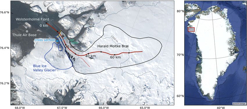
3358                                                                                      L. Müller et al.: Surges of Harald Moltke Bræ

Figure 1. Region of investigation as viewed in a Landsat 8 scene of August 2014 (USGS, 2019) (see red box in the right image for its
location in Greenland). Blue and black lines mark the drainage basins of Blue Ice Valley Glacier and Harald Moltke Bræ, respectively. Red
lines (solid and dashed) mark the approximate centre line of the main glacier stream and of a tributary, respectively. The starting point of the
centre line is at the mean position of the glacier front line in 1916 (year of the first available record of the front position). We use the glacier
front position of 1916 as a reference for all longitudinal profiles and glacier front positions. The yellow line marks the approximate front
positions of 2020. The black triangle marks the point (67.628◦ W, 76.588◦ N) to which all velocity time series in this paper refer.

Table 1. Overview of the technical details of the velocity data sets from Landsat, Sentinel-1 (D), Sentinel-1 (P) and TerraSAR-X. The velocity
fields are given in the form of regular spatial grids. The time basis refers to the acquisition time difference of the image pairs used for the
velocity determination. The time difference denotes the interval between two consecutive velocity fields.

                           Data set                  Landsat          Sentinel-1 (D)     Sentinel-1 (P)    TerraSAR-X
                           Time span                 1998–2018        2014–2018          2016–2020         2011–2017
                           Spatial resolution (m)    150–600          300                500               100
                           Time basis (d)            5–100            12                 12                11
                           Time difference (d)       1–16             12                 6/12              11–351
                           Source                    TU Dresden       DTU Space          PROMICE           NSIDC

1 km (Noël, 2019). We average the SMB, precipitation and                    4     Results
runoff over a fixed area, which is defined as the part of the
glacier basin up-glacier of the cross section at about 16 km                4.1    Flow velocity time series near the glacier front
(Fig. 1). Additionally, we compute the ice-mass flux through
this cross section. Therefore, we determine a cross-sectional               Figure 2 shows the velocity variations in time, observed at
profile of surface velocities scaled by a factor of 0.9. At each            a fixed position close to the terminus (Fig. 1). Ice flow ac-
point of this profile, the mass flux through a vertical column              celerated significantly in 1999/2000 and 2005/2006 and in
in the glacier is computed using ArcticDEM and BedMa-                       2013–2019. During the 2013–2019 phase, the dense tempo-
chine. By summing up the resulting mass fluxes, we approx-                  ral sampling reveals pronounced seasonal velocity variations
imate the total flux through the cross-sectional area.                      by 1 order of magnitude. At the end of 2019, velocities re-
                                                                            turned to a very low level that was sustained at least until
                                                                            July 2020.
3.6    Visible features
                                                                            4.2    Front position
We also assess changes traceable by visual inspection of the
Landsat scenes. We focus on four different features: lakes                  Figure 3 shows that most of the active phases between 1916
on the glacier surface, outflow of subglacial meltwater at                  and 2020 were accompanied by an advance of the terminus
the glacier front (meltwater plumes), sea ice coverage in                   which interrupted its long-term retreat (Mock, 1966). From
the fjord, and calving events (Appendix E). We assess these                 1926 to 1928 the frontal advance was more pronounced than
features by distinguishing between three states: not visible,               in later active phases. During the surge event in 1954–1956,
moderate and strong occurrence.                                             the glacier front retreated slightly.

The Cryosphere, 15, 3355–3375, 2021                                                                https://doi.org/10.5194/tc-15-3355-2021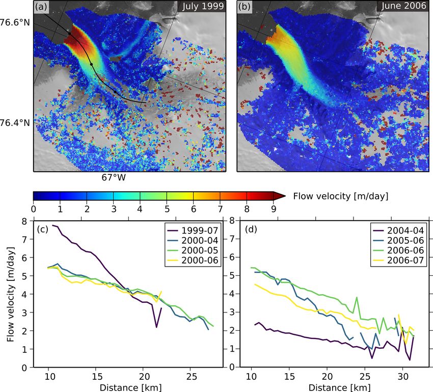
L. Müller et al.: Surges of Harald Moltke Bræ 3359
Figure 2. Flow velocity for the time period from January 1998 to July 2020 derived from Landsat, Sentinel-1, and TerraSAR-X at a point
close to the terminus of Harald Moltke Bræ. For Sentinel-1 we use two different velocity data sets: one processed at Denmark’s National
Space Institute (DTU Space), referred to as Sentinel-1 (D), and another one provided by the Programme for Monitoring of the Greenland Ice
Sheet (PROMICE), referred to as Sentinel-1 (P).
lower than the calving rate. In the years before the surge
2005/2006, this retreat was about 500 m yr−1 . In the active
phases, the glacier front advances by about 500 m yr−1 , indi-
cating that the flow velocity exceeds the calving rate.
Generally, no clear correlation between interannual varia-
tions of flow velocities and external influences (precipitation,
runoff and SMB) could be identified (Fig. 4). Due to excep-
tionally high precipitation the SMB peaks in 2004 shortly
before the initiation of the surge in spring 2005. The basin
average annual SMB is negative after the termination of the
surge in 2006 due to increased meltwater runoff. This im-
plies that after 2006 the glacier loses mass even without ice
discharge by calving.
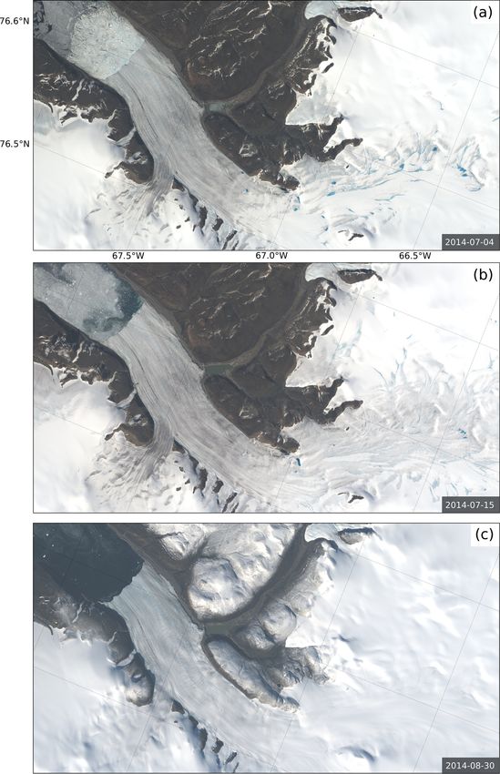
Figure 3. Average front position with respect to the terminus of The velocity fields visualized in Fig. 5 show that in both
1916 consistent with the profile line shown in Fig. 1. The docu- active phases, 1999/2000 and 2005/2006, the velocities were
mented surges are marked by light blue colour. highest at the glacier front and decreased approximately lin-
early with increasing distance from the front. As indicated in
Fig. 5c and d, shortly after the surge initiation (July 1999 and
Besides documented surge events, there are further phases June 2005), fast ice flow is found, especially in the lower part
of frontal advance between 1970 and 1985 for which, how- of the glacier associated with steeply sloped velocity profiles.
ever, independent velocity observations are not available. Towards the end of a surge (e.g. June 2000 and July 2006),
Further, Fig. 3 indicates a long-term acceleration of the however, upper parts of the glacier were increasingly affected
frontal retreat rate from about 100 m yr−1 before 2000 to by fast ice flow, whereas the velocities were decreasing close
about 200 m yr−1 thereafter (approx. 8 km between 1920 and to the terminus.
2000 compared to approx. 4 km between 2000 and 2020).
4.4 Ice flow during the active phase 2013–2019
4.3 Ice flow during the active phases 1999/2000 and
2005/2006 In autumn/winter 2013 there was an abrupt change from con-
stantly low velocities of less than 1 m d−1 in all months with
In both active phases, 1999/2000 and 2005/2006, the glacier available data to pronounced seasonal fluctuations over an
exhibits high velocities (> 4 m d−1 ) in late spring (Fig. 4). order of magnitude with maximum velocities of 6–10 m d−1
There is a rapid acceleration in spring 2005 and a rapid slow- in spring and summer (Fig. 6). While the velocities dropped
down in summer 2006. In the years 2001, 2004 and 2007, well below 1 m d−1 in summers 2014, 2015 and 2016, they
which are before or after surge periods, an acceleration in remained on a medium level above 1 m d−1 in summers 2017
spring and peak velocities in early summer are also visible. and 2018.
Over most of the rest of the quiescent phases the flow veloc- The front retreated by 1000 m yr−1 between 2011 and
ities remain clearly below 1 m d−1 with no significant fluctu- 2013 (Fig. 6), faster than in the previous quiescent phases
ations. (500 m yr−1 ), possibly due to a long-term increase in the
During the quiescent phases the glacier front retreats calving rate. Due to this frontal retreat the constant point to
(Figs. 3, 4), indicating that the flow velocity at the front is which the velocities in Fig. 6 refer is located closer to the
https://doi.org/10.5194/tc-15-3355-2021 The Cryosphere, 15, 3355–3375, 2021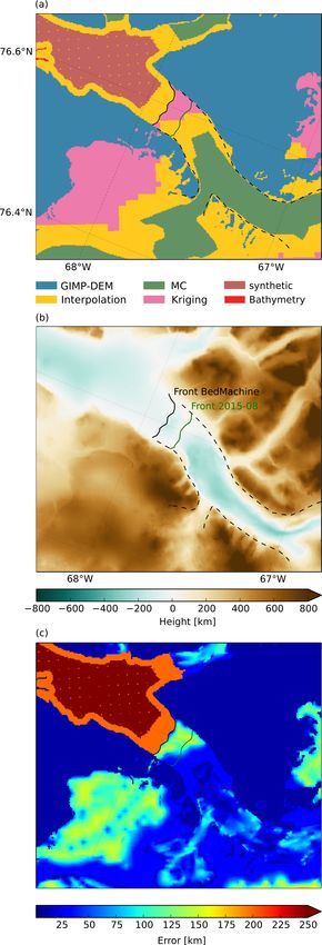
3360                                                                                 L. Müller et al.: Surges of Harald Moltke Bræ

Figure 4. (a) Yearly precipitation, meltwater runoff and SMB averaged over the drainage basin. (b) Monthly front position with respect to
the year 1916 digitized in Landsat images where available. (c) Monthly glacier velocity and its uncertainty estimate derived from the Landsat
data set at a point close to the terminus of Harald Moltke Bræ (black triangle in Fig. 1). The surges are marked by light blue colour.

front in 2013. We note that this closer location to the glacier          increased velocities already in September 2013. Between
front could be one reason for the higher maximum velocity                April and July 2014, the ice flow was slowing down from
in 2013 compared to previous surges. However, it cannot be               month to month between 13 and 22 km, whereas it was con-
the main cause of the increase in flow velocities by 1 order             tinuing to accelerate further upstream. After the slowdown
of magnitude in 2013, since the acceleration in 2013/2014                between July and August 2014, the glacier had the lowest ve-
affects the entire part between 13 and 25 km (Fig. 7). The               locities at the glacier front and a velocity maximum at about
high average velocity between 2013 and 2015 exceeded the                 29 km, unlike September 2013.
calving rate and led to a rapid advance of the glacier front.               The cross velocity profiles in Fig. 7f show that both
Thereafter the terminus retreated on average by 200 m yr−1 ,             streams, the main stream of Harald Moltke Bræ and the
since the rather short-term accelerations in 2016 and 2017               part of Blue Ice Valley Glacier, were equally affected by the
were not sufficient to compensate for the calving rate.                  surge. Thus, the velocity changes had a uniform effect over
   The average SMB was exceptionally high (10 kg m−2 d−1 )               almost the entire width of the glacier.
in 2013, the year of surge initiation. In contrast to the SMB               Two distinct patterns of seasonal ice flow variations can
maximum in 2004, the SMB maximum in 2013 is due to a                     be identified in Fig. 8a. In 2014, 2015 and 2018, the glacier
low meltwater runoff rather than a high accumulation rate.               reached high velocities of more than 4 m d−1 already be-
   Directly before (September 2013) and after (August 2014)              tween January and March. By contrast, in 2016 and 2017, the
a phase of accelerated ice flow, the velocities were about               velocities remained below 2 m d−1 in autumn and increased
1 m d−1 or less over almost the entire glacier (Fig. 7). A               only gently at the beginning of the year, followed by a rapid
slight acceleration already occurred in July and August 2013             acceleration between May and June. The rapid slowdown in
(Fig. 6). From September to December 2013 the velocities                 summer around July and August is common to all years be-
increased rapidly in the part below 20 km, whereas the parts             tween 2013 and 2018. These decelerations coincide with the
further upstream were less affected or not affected at all. Sub-         maximum of the meltwater runoff (Fig. 8b).
sequently, the upper parts of the glacier also accelerated sig-             The longitudinal velocity profiles for July of the years
nificantly, leading to velocities of more than 5 m d−1 within            2015 to 2018 (Fig. 9a) all show a similar decrease from about
most of the glacier area below 25 km.                                    6.5 m d−1 at 14 km to about 2 m d−1 at 31 km.
   The longitudinal profiles in Fig. 7e show that a small part              In contrast to July, the profiles for September vary largely
at the glacier front with an extension of 2–3 km had slightly            over the years 2015 to 2018 (Fig. 9b). In 2015 and 2016, ve-

The Cryosphere, 15, 3355–3375, 2021                                                           https://doi.org/10.5194/tc-15-3355-2021
L. Müller et al.: Surges of Harald Moltke Bræ 3361
Figure 5. Exemplary velocity fields (a, b) and velocity profiles (c, d) for the surges 1999/2000 and 2005/2006. The profile location is shown
as a black line in (a), with black circles every 10 km along the profile. The starting point of this line is the glacier front position of 1916. The
background image in (a, b) is a Landsat 8 scene (USGS, 2019).
locities remained relatively low and had their maximum at the formation of meltwater plumes at the glacier front. Melt-
approximately 29 km. In 2017 and 2018 (years with rapidly water plumes were larger in the active phase 2013–2019 than
increasing velocities in autumn), velocities were highest at between 2011 and 2013. However, the extent of supraglacial
the glacier front. In 2015, 2016 and 2017, ice flow was en- lakes on the glacier surface was about the same before and
hanced within 2–3 km from the terminus. after 2013. In contrast to the supraglacial lakes, the station-
ary lake at the northern side of the glacier does not exhibit
4.5 Ice flow during the quiescent phases any significant seasonal or long-term variations visible in the
Landsat images.
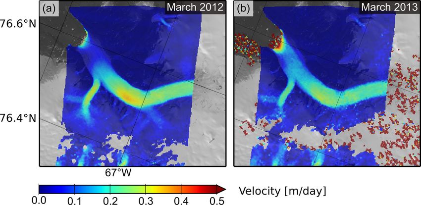
In the quiescent phase, velocity maxima amounted to 0.3– Due to the low resolution of the Landsat images, the for-
0.4 m d−1 in both the main stream of Harald Moltke Bræ mation of crevasses was not analysed. All further remarks on
(about 29 km) and in the Blue Ice Valley Glacier about crevasses are solely based on the assumption that the rapid
2 km upstream from the confluence with Harald Moltke velocity fluctuations involve crevasse formation.
Bræ (Fig. 10). Velocities were lowest (lower than 0.2 m d−1 ) The middle moraine between Blue Ice Valley Glacier and
within an area of about 8 km extent right below the conflu- the main stream of Harald Moltke Bræ, as inspected from
ence. Within 2–3 km from the terminus, however, velocities the Landsat images, does not show any significant change in
were slightly higher, at about 0.3 and 0.5 m d−1 in March position or surge looped geometry (Appendix E), even during
2012 and March 2013, respectively. phases of highly variable flow velocities. This indicates that
both glaciers were identically involved in the surge.
4.6 Visually inspected features
4.7 Ice-mass balance
In years with high flow velocities (2014–2018), both calv-
ing events and the sea ice break-up in the fjord started ear- The time series of the mass flow through a cross-sectional
lier compared to the preceding quiescent phase (Fig. 11). area close to the glacier front (Fig. 12) has three clear steps
Supraglacial lakes always formed in summer, followed by marking the surge events. During the surge phases, the esti-
https://doi.org/10.5194/tc-15-3355-2021 The Cryosphere, 15, 3355–3375, 2021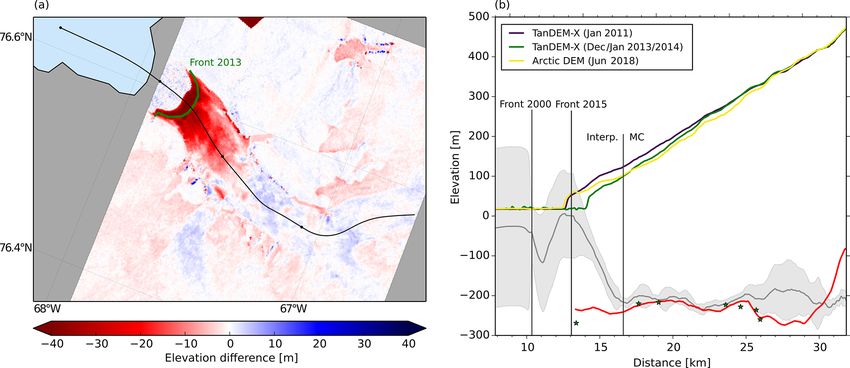
3362                                                                                 L. Müller et al.: Surges of Harald Moltke Bræ

Figure 6. (a) Yearly precipitation, meltwater runoff and SMB averaged over the drainage basin. (b) Monthly front position with respect to
the year 1916 digitized in Landsat images where available. (c) Monthly glacier velocity and its uncertainty estimate derived from the Landsat
data set at a point close to the terminus of Harald Moltke Bræ (black triangle in Fig. 1). Red error bars indicate the standard deviations of
monthly velocity values from different data sets. The surges are marked by light blue colour.

mated average ice-mass discharge was 0.5–1 Gt yr−1 subject               high level of 100 m. From 13 km up-glacier the BedMachine
to uncertainties associated with the interpolation of flow ve-           bedrock declines steeply to a depth of 200 m at 16 km with an
locities to unobserved months. During the quiescent phases,              uncertainty of 10–20 m (Morlighem et al., 2017). However,
mass flux was mostly below 0.05 Gt yr−1 . The average SMB                between 13 and 16 km, CReSIS data deviate significantly
was roughly 0.2 Gt yr−1 in 1990–1998 and 0.1 Gt yr−1 in                  from BedMachine and suggest a gently sloped bedrock with
2001–2004. Thus, between 1998 and 2006, the ice discharge                a depth of about 230 m at the front position of the year 2015.
exceeded SMB during the active phases, while SMB ex-                     From 16 to 25 km the BedMachine–CReSIS differences vary
ceeded discharge during the quiescent phases. After 2006,                between 5 and 100 m, on the level of the uncertainties speci-
however, both the ice flux and SMB contribute to an overall              fied for BedMachine (Morlighem et al., 2017).
mass loss of about 0.4 Gt yr−1 . SMB maxima in 2004 and                     Below a distance of 16 km only interpolation methods
between autumn 2012 and spring 2014 precede the active                   were used in BedMachine (see Appendix C). Independent
phases 2005/2006 and 2013–2019.                                          CReSIS observations are in good agreement with each other
                                                                         (see crossovers in Fig. 13). Thus, we assume that CReSIS
4.8    Bedrock and ice surface geometry                                  provides a more accurate representation of the true bedrock
                                                                         topography close to the terminus and that the BedMachine
We examined the bedrock topography from BedMachine                       sequence of a trough and a ridge at 10–12 and 13 km, respec-
(Morlighem et al., 2017) and from CReSIS, both along the                 tively, are an interpolation artefact.
same CReSIS flight path (Fig. 13). BedMachine suggests a                    Surface elevations and elevation changes are also shown
trough at 10–12 km (close to the front position of the year              in Fig. 13. The difference between the 2013/2014 and 2011
2000) and a ridge at about 13 km (close to the front posi-               TDM DEMs (Fig. 13a) reveals a significant ice thinning
tion in 2015) associated with an ice thickness as low as 40 m.           close to the glacier front by up to 30 m in the 3 years preced-
The BedMachine uncertainty in this section is specified at a

The Cryosphere, 15, 3355–3375, 2021                                                           https://doi.org/10.5194/tc-15-3355-2021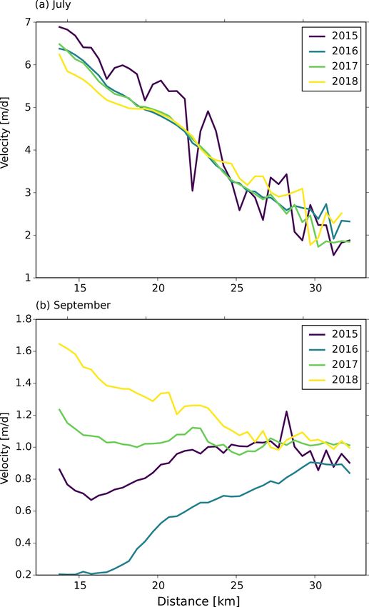
L. Müller et al.: Surges of Harald Moltke Bræ                                                                                           3363

Figure 7. (a–d) Velocity fields for four selected months within the period from September 2013 to August 2014. The background image is a
Landsat 8 scene (USGS, 2019). (e, f) Longitudinal and cross velocity profiles for the same year. Profile locations are shown in panel (a). The
line marking the longitudinal profile location starts at the glacier front position of 1916 (same as in Fig. 5).

ing the 2013–2019 surge, whereas parts further up-glacier at             before the surge initiation in 2013, the spatial distribution of
30 km slightly thickened by an average of about 1–2 m. As a              flow velocities induced a rather slow dynamic thinning of the
consequence, the glacier surface was steepening (Fig. 13b).              glacier tongue between 14 and 20 km and a slow thickening
Between 2013 and 2018, however, the glacier advanced and                 further up-glacier. The pattern of thinning near the terminus
thickened in a small area at the terminus (Fig. 13b), so that            is amplified to values of up to 2 m per month in Septem-
there the surface slope became gentler again. Thus, the ge-              ber 2013, shortly before the surge initiation. In December
ometry near the glacier front in 2018 was similar to that in             2013 the extremum of surface lowering has moved further
2011. At the same time, the ice surface height between 17                upstream (to 20 km) and has reached a value of −4 m per
and 24 km decreased from winter 2013/2014 to 2018.                       month. In spring 2014, the massive acceleration of the en-
   Monthly profiles of dynamic ice-height changes along a                tire lower part of Harald Moltke Bræ up to 25 km entails a
flow line are shown in Fig. 14. During the quiescent phase               rapid dynamic increase in surface height (3–6 m per month)

https://doi.org/10.5194/tc-15-3355-2021                                                          The Cryosphere, 15, 3355–3375, 2021
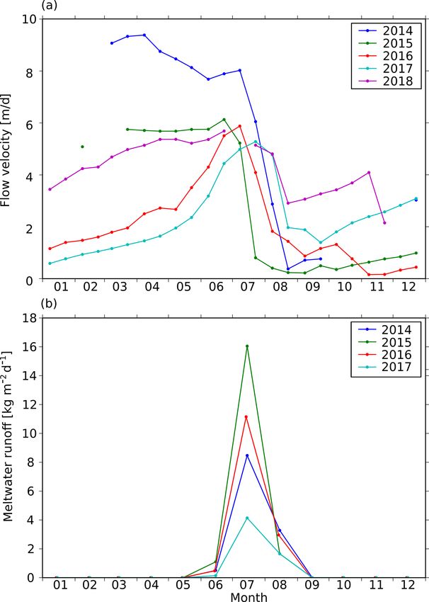
3364                                                                               L. Müller et al.: Surges of Harald Moltke Bræ

Figure 8. Seasonality of flow velocities (semi-monthly velocities at
the point marked by the black triangle in Fig. 1) (a) and meltwater
runoff (b). For 2018, data of meltwater runoff were not available.

in the lowest 5 km of the glacier and a rapid thinning (−8 to          Figure 9. Longitudinal velocity profiles for always a month with
−6 m per month) further up-glacier. During spring 2014 this            high velocities (July) (a) and a month with low velocities (Septem-
pattern appears to propagate upstream.                                 ber) (b). The distance is measured from the 1916 glacier front posi-
   The accelerations of 2014/2015 and 2015/2016 (Fig. 15)              tion.
differ from those of 2013/2014 as they were not preceded by
a rapid thinning. The dynamic height changes in 2014/2015
and 2015/2016 indicate overall a simultaneous acceleration             surges. In 1999, 2000 and 2005, any possible deceleration
of the glacier rather than an up-glacier propagation.                  in July/August would have remained unobserved due to the
                                                                       lack of velocity data. In 2006 and 2007, flow velocities in-
                                                                       deed decreased rapidly in summer, similarly to 2013–2019
5   Interpretation and discussion                                      (Figs. 4 and 6). Using the same data as the present study, yet
                                                                       at a different position, Rosenau (2014) showed that the ve-
The flow velocity variations of Harald Moltke Bræ exhibit              locities close to the terminus had decreased below 1 m d−1
at least two different signals: episodic surges and a season-          before they increased again in 2007. The rapid acceleration
ality with velocities abruptly decreasing in summer. For the           in spring 2005 and the velocity peaks in summers 2001, 2004
identification of the surge periods, as mentioned in Sect. 1,          and 2007 are consistent with a seasonality that is character-
we use both the strong change in flow velocity and the termi-          ized by maximum velocities in spring and early summer. Po-
nus advance as the main criteria (Sevestre and Benn, 2015).            tentially, a seasonality of smaller amplitude was also present
The occurrence of a pronounced seasonality in velocity si-             during the quiescent phases but could not be identified due to
multaneously with a surge can be identified for the period             the limited accuracy of the Landsat velocity fields. Thus, our
2013–2019 (Figs. 2 and 6). It would be conceivable that sim-           main hypothesis for the explanation of the surge behaviour
ilar seasonal velocity changes were present during previous            of Harald Moltke Bræ is as follows: the effect of seasonally

The Cryosphere, 15, 3355–3375, 2021                                                         https://doi.org/10.5194/tc-15-3355-2021
L. Müller et al.: Surges of Harald Moltke Bræ 3365
Figure 10. Exemplary velocity fields during a quiescent phase in March 2012 and 2013. The background image is a Landsat 8 scene (USGS,
2019). The colour scale is different from that in the previous figures.
Figure 12. Cumulated mass flow through a cross section of Har-
ald Moltke Bræ close to the terminus (blue) and monthly cumu-
lated SMB (green) summed over the drainage basin. The surges are
marked by light blue colour.
changing external influences on ice dynamics is episodically
amplified due to internal feedback mechanisms.
5.1 Types of seasonal velocity variations
We distinguish three different types of seasonality (a)–(c) at
Harald Moltke Bræ: (a) in some years (e.g. 2016 and 2017),
there were low and rather gently increasing velocities at the
beginning of the year, followed by a more pronounced accel-
eration from the onset of the melt season (Fig. 8). Despite a
significantly lower amplitude, the seasonality of 2001, 2004
and 2007 may also be consistent with type (a). (b) In 2014
and 2015, for instance, the velocities were already high at the
beginning of the year (as they increased in autumn of the pre-
vious year) and remained high over several months in spring
(Fig. 8). In both cases (a) and (b), the flow velocities decrease
Figure 11. Occurrence of four different visual features from 2011 rapidly in July or August. (c) During most of the quiescent
to 2017. Examples for the assessment of these visual features in phase, the velocities remained below 1 m d−1 . A significant
Landsat scenes are given in Appendix E. variation in quiescent velocities cannot be detected either be-
cause it does not occur or because of the limited accuracy of
the Landsat data.
https://doi.org/10.5194/tc-15-3355-2021 The Cryosphere, 15, 3355–3375, 20213366 L. Müller et al.: Surges of Harald Moltke Bræ
Figure 13. (a) Difference between ice surface elevations from two TanDEM-X observations (December/January 2013/2014 minus January
2011). (b) Profiles of bedrock topography from BedMachine (grey) and CReSIS (red) along the ground track of a flight path from May 2014
(Paden et al., 2019). Stated uncertainties for the BedMachine data set (Morlighem et al., 2017) are indicated by the grey error band. Green
stars mark the elevations from independent CReSIS measurements at the intersections of the ground tracks. Vertical lines mark the front
positions of 2000 and 2015 and the boundary between the areas where BedMachine applied interpolation and a mass conservation approach
(MC), respectively (Morlighem et al., 2017). Profiles of glacier surface height at different times are also shown. Panel (a) also shows the
profile location (black line starting at the glacier front position of 1916 and black circles every 10 km along the profile) and the front position
of December/January 2013/14 (green line).
drainage system (Moon et al., 2014; Vijay et al., 2019). Sim-
ilarly to that, there may be a transition from an inefficient
to an efficient subglacial drainage system in July/August in
years with a seasonality of our type (a) or (b).
Some additional observations indicate a hydrological con-
trol on the seasonality at Harald Moltke Bræ: the formation
of large supraglacial meltwater lakes at the beginning of the
summer when velocities are highest (see the example in Ap-
pendix E), the occurrence of a meltwater plume shortly there-
after, the speedup at the onset of the melt season, and, further,
the short-lived accelerations of ice flow right before the slow-
down in 2014 and 2015 as a presumed effect of enhanced
Figure 14. Dynamically caused ice-height changes derived from basal water pressure which subsequently leads to the forma-
velocity profiles along a flow line (as marked in Fig. 5). The distance tion of an efficient drainage system.
is measured from the 1916 glacier front position. According to Moon et al. (2014), type (3) differs from (2)
in autumn as there is still enough meltwater available to raise
the water pressure significantly and, thus, to accelerate the
5.2 Seasonal mechanism ice flow. At Harald Moltke Bræ, we find a rather converse
relationship: compared to years with low meltwater runoff
Type-(a) and -(b) behaviours correspond to the seasonality of (e.g. 2017), in years with larger meltwater runoff the ice flow
the glacier types (2) and (3), respectively, identified by Moon slows down a bit earlier (already in July instead of August),
et al. (2014) and Vijay et al. (2019) (Sect. 1). Harald Moltke the velocities decrease to a lower level and the deceleration
Bræ switches between type-2 and type-3 behaviours. Fur- is not directly followed by a rapid velocity increase in au-
ther, during the surges, the seasonal variations being about tumn (leading to type a in the following year) (Fig. 8). Po-
6 m d−1 clearly exceed the fluctuations of about 1–2 m d−1 tentially, more meltwater leads to a more efficient subglacial
observed by Moon et al. (2014). drainage system that prevails for a longer time in the year so
The deceleration of type-2/3 glaciers during the late melt that less meltwater is trapped at the glacier base in autumn.
season is correlated with the maximum of meltwater runoff, Consequently, the comparably less pronounced decelerations
indicating a transition from an inefficient to a channelized
The Cryosphere, 15, 3355–3375, 2021 https://doi.org/10.5194/tc-15-3355-2021L. Müller et al.: Surges of Harald Moltke Bræ 3367
Figure 15. Dynamically caused ice-height changes derived from velocity profiles along a flow line for selected months during ice flow
acceleration 2014/2015 (a) and 2015/2016 (b). The distance is measured from the 1916 glacier front position.
in 2017 and 2018 may be interpreted as an effect of lesser 1928 and 1954–1956 were significantly different from the
amounts of meltwater runoff. more recent surges.
5.4 Classification of flow patterns
5.3 Is the surge 2013–2019 different from previous
surges? We distinguish between four different flow patterns (A–D)
based on the spatial distribution of flow velocities. Each pat-
There are several similarities between the surges 1999/2000 tern is associated with a certain profile of dynamic ice-height
and 2005/2006: a duration of 2 years (years with velocities changes and, thus, has certain consequences for the stresses
exceeding 4 m d−1 ), persisting high velocities over at least and the mass redistribution in the glacier system.
3 months in the second year of the surge (2000 and 2006) (A) A first pattern is characterized by low velocities (<
(Fig. 5), and a year with slightly enhanced summer veloci- 0.3 m d−1 ) in the lower part of the glacier and moderately
ties following the surge. By contrast, the surge 2013–2019 higher velocities further upstream. This causes only minor
had at least 6 years with velocities exceeding 4 m d−1 . Fur- dynamically induced changes in the receiving area and a dy-
ther, the surge 2013–2019 was initiated by an abrupt acceler- namic thickening in the reservoir area (Fig. 16). This pattern
ation in autumn/winter reaching velocities of up to 10 m d−1 , can be found for many of the quiescent phases, e.g. in March
whereas the surge 2005/2006 began with an acceleration 2012 (Fig. 10a). In pattern (B), the glacier exhibits low flow
in spring 2005. It is likely that all three observed surges, velocities (< 0.5 m d−1 ) over most of its area except for a
1999/2000, 2005/2006 and 2013–2019, were modulated by small part at the front where the velocities exceed 1 m d−1
a similar mechanism of seasonality. (Fig. 16). This pattern arises shortly before the surge initi-
It must be considered that – before 2013 – the flow vari- ation, e.g. in September 2013 (Fig. 7). Thus, a pronounced
ability may be underestimated due to data gaps and larger thinning occurs directly at the glacier front. (C) A third pat-
time bases (Appendix A) which involve large smoothing ef- tern has a steeply sloped velocity profile (with a maximum
fects. Due to the retreat of the glacier front, the fixed refer- of about 6–10 m d−1 at the glacier front) in the lower 10 km
ence point for the velocities was closer to the glacier front of the glacier, whereas larger parts further upstream remain
in 2013 than at the times of previous surges. This is likely at low velocities similar to patterns (A) and (B) (Fig. 16).
one reason why velocity peaks in 2013 to 2019 are higher This was the case in December 2013 (Fig. 7), for instance.
than during previous surges. Thus, the surges 1999/2000, This pattern may be associated with only moderate height
2005/2006 and 2013–2019 might be more similar than sug- changes at the glacier front and in the upper parts of the
gested at first glance in Figs. 2 and 6. However, in terms of its glacier, whereas the middle part of the glacier is rapidly thin-
duration, the most recent surge clearly differs from the surges ning (Figs. 14 and 16). This results in a decrease in surface
1999/2000 and 2005/2006. slope at the terminus and a significant increase in surface
As the observed accelerations 1926–1928 and 1954–1956 slope in the middle part. (D) The fourth pattern shows high
refer to the average over a period of 2 years, the true max- velocities at the glacier front, similar to pattern (C). (D) dif-
imum velocities are probably significantly higher than the fers from (C) in that it has higher velocities in the middle
documented velocities of 3.6 and 1 m d−1 , respectively. In and upper parts of the glacier (Fig. 16). This is associated
addition, the exact timing of the surges is unknown. They with a more gently sloped velocity profile in the lower 10 km
may have lasted longer or shorter than 2 years. In summary, of the glacier. As a consequence, the glacier is dynamically
there are not enough data to state whether the surges 1926– thickening in its lower part and thinning in its upper part. Pat-
https://doi.org/10.5194/tc-15-3355-2021 The Cryosphere, 15, 3355–3375, 20213368 L. Müller et al.: Surges of Harald Moltke Bræ
clude that once the entire glacier has accelerated, large parts
of the glacier are set into a condition to accelerate again in
the following years.
5.6 Glacier geometry during the quiescent phases
Similarly to other surge-type glaciers, the quiescent phase of
Harald Moltke Bræ is characterized by slower flow in the
lower part and faster flow in the upper part. However, the
transition between slower and faster flow is rather smooth,
which implies just a slight dynamic thickening (a few metres
over 3 years; see Fig. 13). We therefore hypothesize that for
the initiation of the surge, the increase in driving stresses in
this transition zone is less important than the decrease in re-
sisting stress at the glacier front implied by the frontal retreat.
The findings are opposite to down-glacier propagating surges
e.g. observed at Variegated Glacier (Raymond, 1987) and
at Bivachny Glacier (Wendt et al., 2017). The pronounced
thinning at the glacier front is compatible with an up-glacier
Figure 16. Schematic representation of the velocity and the corre-
sponding dynamic ice-height changes for the patterns (A), (B), (C)
propagating surge observed at Aventsmarksbrae (Sevestre et
and (D). al., 2018). Thus, a significantly larger thinning at the glacier
front compared to a lesser thickening in the upper part of the
glacier could be a key factor for the surge initiation at the
terminus and an up-glacier propagation.
tern (D) reverses the combined effect of patterns (A) and (B),
however, with a difference in magnitude. Thus, the effect of
the longer-lasting quiescent phase can be compensated for by 5.7 Potential causes and triggers of the surges
a shorter-lasting active phase. Pattern (D) can be found e.g.
in the velocities of spring and early summer 2014 (Fig. 7). On long timescales, the dynamics of Harald Moltke Bræ may
During the initiation of the surge 2013–2014, these flow be determined by externally driven influences such as SMB
patterns followed each other in the sequence (A)–(B)–(C)– and the long-term retreat of the glacier front. On the interan-
(D). Similarly to winter 2013/2014, the velocity profiles in nual timescale, however, the flow velocity does not react si-
1999 and 2005 (first year of the surge) were also steeper than multaneously to external drivers such as the terminus retreat
in the following years 2000 and 2006 (second year of the and the cumulated SMB. Instead, local conditions might re-
surge). Hence, there might have been a similar sequence (A)– strict the ice flow during the quiescent phase and facilitate an
(B)–(C)–(D) initiating all surges. This sequence reflects an increasing instability that finally results in a surge.
evolution of dynamic changes within the glacier where first, Several factors may potentially restrict the ice flow in the
through pattern (B), mass from the middle part of the glacier lower part of the glacier during a quiescent phase: a cold
is mobilized to compensate for the mass deficit at the glacier glacier base that is partly frozen to the glacier bed (cor-
front leading to (C). Subsequently, the surplus of mass in the responding to the thermally driven mechanism, maybe re-
upper part of the glacier is set in motion to compensate for lated to strengthened subglacial till), a subglacial drainage
the mass deficit in both the middle and lower parts, resulting system remaining efficient over several years (correspond-
in pattern (D). ing to the hydrologically driven mechanism), a bump in the
In the years after the surge initiation, the sequence appears bedrock topography, a dynamic interaction of Blue Ice Valley
to be different. There is a rather direct switch between (A) Glacier and Harald Moltke Bræ, and the absence, or closure,
and (D), whereas the patterns (B) and (C) are largely absent of crevasses preventing meltwater from reaching the glacier
(Fig. 15). base.
Wendt et al. (2017) discussed a bump in the glacier bed
5.5 Up-glacier propagation of the surges as the cause of restricted ice flow during the quiescent phase
of Bivachny Glacier. At Harald Moltke Bræ, there is a bump
The sequence of patterns (A)–(B)–(C)–(D) is consistent with at about 25 km according to the CReSIS data set, which is,
an up-glacier propagation of the surge. In the consecutive however, small compared to the ice thickness. Closer to the
years, however, the direct switch between (A) and (D) re- terminus, the large uncertainties of the BedMachine data set
flects a rather uniform acceleration of most of the ablation do not allow us to identify relevant features of the bedrock
zone of Harald Moltke Bræ. Based on these findings, we con- topography.
The Cryosphere, 15, 3355–3375, 2021 https://doi.org/10.5194/tc-15-3355-2021L. Müller et al.: Surges of Harald Moltke Bræ 3369 The presence of a seasonality parallel to surges has been cle. The 2013–2019 surge and its preceding quiescent phase taken as a clear indicator of a hydrologically driven mecha- lasted longer (5 and 6 years) than the surge and the quiescent nism at other glaciers (Wendt et al., 2017; Raymond, 1987). phase in the preceding cycle (5 and 2 years, respectively). Furthermore, the rapid onset of the surge in 2013 suggests This could be related to the SMB in the drainage basin being a hydrological mechanism. By contrast, a thermally driven negative after 2006. Also, the intermediate annual retreat of mechanism is typically characterized by a rather gradual the glacier front in 2016 and 2017 could have prevented the surge initiation (Murray et al., 2003; Jiskoot, 2011). A ther- glacier from stabilizing such that in 2018 and 2019 velocities mally driven mechanism is also unlikely, as the intermediate of more than 4 m d−1 are still reached. decelerations during summer, when the glacier goes back to a state similar to the quiescent phase, cannot be explained by an abrupt freezing of the glacier base or a strengthening 6 Conclusions of subglacial sediments. Therefore, the hydrologically driven mechanism provides an overall more plausible explanation By combining four different remotely sensed velocity data for the surges at Harald Moltke Bræ than a thermally driven sets, we estimated a monthly velocity time series for Harald mechanism. Moltke Bræ with high spatial and temporal resolution. Based The surges of Harald Moltke Bræ may develop as follows: on this time series we identified mainly two different signals during the quiescent phase, the combined effect of low flow of velocity variations close to the terminus of Harald Moltke velocities and a negative mass balance in the ablation zone Bræ: episodic surges and a pronounced seasonality. As we involves a thinning and steepening of the glacier tongue and assume that there is a similar seasonality in most years of the a retreat of the glacier front. Observations from CReSIS in- observation period, we interpret the surges as phases with a dicate a rather thick marine-terminating glacier front of more strongly amplified seasonal amplitude. than 200 m which could facilitate the thinning and the retreat. The annual flow velocities of Harald Moltke Bræ were These factors may lead to a decrease in resisting forces at high over a relatively long period of 6 years from 2013 to the terminus. Additionally, at a thick glacier, the steepening 2019, which has not been observed in this way before. How- of the glacier due to thinning at the terminus could increase ever, flow velocities remaining low in autumn/winter 2019 the driving stress (Sevestre et al., 2018). The resulting large and spring 2020 indicate the beginning of a new quiescent net stress in the flow direction may cause a small area at the phase. Thus, the high velocities between 2013 and 2019 may glacier front to accelerate (flow pattern B). This induces dif- constitute a longer surge than previous ones but no funda- ferent effects that facilitate a further acceleration and the up- mental change in the flow regime. We therefore assume that ward propagation of the surge: crevassing of the ice surface Harald Moltke Bræ is likely to maintain its surge behaviour. enabling more meltwater to reach the glacier base (Sevestre Regarding temporal velocity variability, we identified et al., 2018), weakening of subglacial till (deformation of the types of seasonality which indicate a hydrological control of glacier bed), longitudinal stresses (tension) and a further sur- the seasonal velocity changes. The time of a rapid decelera- face thinning/steepening. As a result, the glacier may change tion in July or August suggests a switch between an ineffi- into pattern (C), which, in turn, transfers these processes fur- cient and an efficient subglacial drainage system due to the ther up-glacier, leading to pattern (D). Once the entire abla- changing amount of meltwater availability. This, however, tion zone of Harald Moltke Bræ was affected by the sequence does not provide an explanation for the significant increase (A)–(B)–(C)–(D), the externally driven seasonal changes in in seasonal amplitude during the surges. meltwater availability could have a more pronounced effect Over the past 2 decades, the overall discharge of the as crevasses have spread over large parts of the glacier and glacier was larger than the overall ice mass accumulation. subglacial till has weakened. Thus, the overall thickness of the glacier was decreasing, This could explain why in years after the year of surge ini- which could be a reaction to the observed long-term retreat tiation there is a simultaneous acceleration of large parts of of Harald Moltke Bræ. However, the glacier does not react the glacier according to a direct flipping between (A) and (D) instantaneously to the terminus retreat by dynamic thinning. rather than an up-glacier propagation. Pattern (D) causes the The reason might be a restricted ice flow during the quiescent ice surface to become more gently sloped. Such a decrease in phases due to internal factors, probably related to the glacial surface slope could stabilize the glacier during the surge and, hydrology. This possibly causes an increasing instability and thus, lead to a reverse feedback: a decreasing annual ampli- results in an alternation of two reverse feedback mechanisms tude causing a gradual closure of the crevasses and, possibly, which involve pronounced acceleration and deceleration, re- a strengthening of the subglacial sediments until the glacier spectively. enters a quiescent phase. Such an evolution is consistent with By distinguishing between different patterns of spatial dis- the velocity peaks in summer 2001 and 2007 following the tribution of flow velocities, we could demonstrate that the surges. surge develops first at the glacier front and that it is propa- Both the SMB and the retreat of the glacier front could de- gating rapidly up-glacier within a few months thereafter. The termine the time of initiation and the length of the surge cy- seasonal amplitude remains high in the years after the year https://doi.org/10.5194/tc-15-3355-2021 The Cryosphere, 15, 3355–3375, 2021
You can also read