Bayesian spatio-temporal inference of trace gas emissions using an integrated nested Laplacian approximation and Gaussian Markov random fields - GMD
←
→
Page content transcription
If your browser does not render page correctly, please read the page content below

Geosci. Model Dev., 13, 2095–2107, 2020
https://doi.org/10.5194/gmd-13-2095-2020
© Author(s) 2020. This work is distributed under
the Creative Commons Attribution 4.0 License.

Bayesian spatio-temporal inference of trace gas emissions using an
integrated nested Laplacian approximation and Gaussian
Markov random fields
Luke M. Western1 , Zhe Sha2,3 , Matthew Rigby1 , Anita L. Ganesan2 , Alistair J. Manning4 , Kieran M. Stanley1,5 ,
Simon J. O’Doherty1 , Dickon Young1 , and Jonathan Rougier3
1 School  of Chemistry, University of Bristol, Bristol, UK
2 School  of Geographical Sciences, University of Bristol, Bristol, UK
3 School of Mathematics, University of Bristol, Bristol, UK
4 Hadley Centre, Met Office, Exeter, UK
5 Institute for Atmospheric and Environmental Science, Goethe University Frankfurt, Frankfurt am Main, Germany

Correspondence: Luke M. Western (luke.western@bristol.ac.uk)

Received: 8 March 2019 – Discussion started: 5 June 2019
Revised: 13 February 2020 – Accepted: 27 March 2020 – Published: 28 April 2020

Abstract. We present a method to infer spatially and spatio-     1   Introduction
temporally correlated emissions of greenhouse gases from
atmospheric measurements and a chemical transport model.
The method allows fast computation of spatial emissions us-      Emissions of greenhouse gases, ozone-depleting substances
ing a hierarchical Bayesian framework as an alternative to       and air pollutants are increasingly inferred indirectly from at-
Markov chain Monte Carlo algorithms. The spatial emissions       mospheric trace gas concentration observations and chemical
follow a Gaussian process with a Matérn correlation structure    transport models. These “top-down” or “inverse” methods
which can be represented by a Gaussian Markov random field       complement inventory- or process-model-based “bottom-up”
through a stochastic partial differential equation approach.     techniques that are used, for example, in national reporting of
The inference is based on an integrated nested Laplacian ap-     greenhouse gas emissions to the United Nations Framework
proximation (INLA) for hierarchical models with Gaussian         Convention on Climate Change (UNFCCC; e.g. Leip et al.,
latent fields. Combining an autoregressive temporal corre-       2018).
lation and the Matérn field provides a full spatio-temporal         Top-down methods rely on some form of statistical in-
correlation structure. We first demonstrate the method on a      ference, or inverse theory, to infer emissions at global (e.g.
synthetic data example and follow this using a well-studied      Saunois et al., 2016) to regional (e.g. Brunner et al., 2017)
test case of inferring UK methane emissions from tall tower      scales. They also require a chemical transport model to pro-
measurements of atmospheric mole fraction. Results from          vide the relationship between atmospheric mole fraction and
these two test cases show that this method can accurately        emissions. The most common type of inverse method uses
estimate regional greenhouse gas emissions, accounting for       Bayesian inference. Bayesian inference relies on the infor-
spatio-temporal uncertainties that have traditionally been ne-   mation about the uncertainties in the measurement, transport
glected in atmospheric inverse modelling.                        model and prior probability of the parameters to inform the
                                                                 emissions estimate. Inverse methods often assume that un-
                                                                 certainties in the likelihood and prior probabilities are known
                                                                 exactly and Gaussian (e.g. Stohl et al., 2009; Brioude et al.,
                                                                 2013). These assumptions allow large inverse problems to be
                                                                 solved efficiently. However, when uncertainties are poorly
                                                                 understood, Bayesian methods have been shown to lead to

Published by Copernicus Publications on behalf of the European Geosciences Union.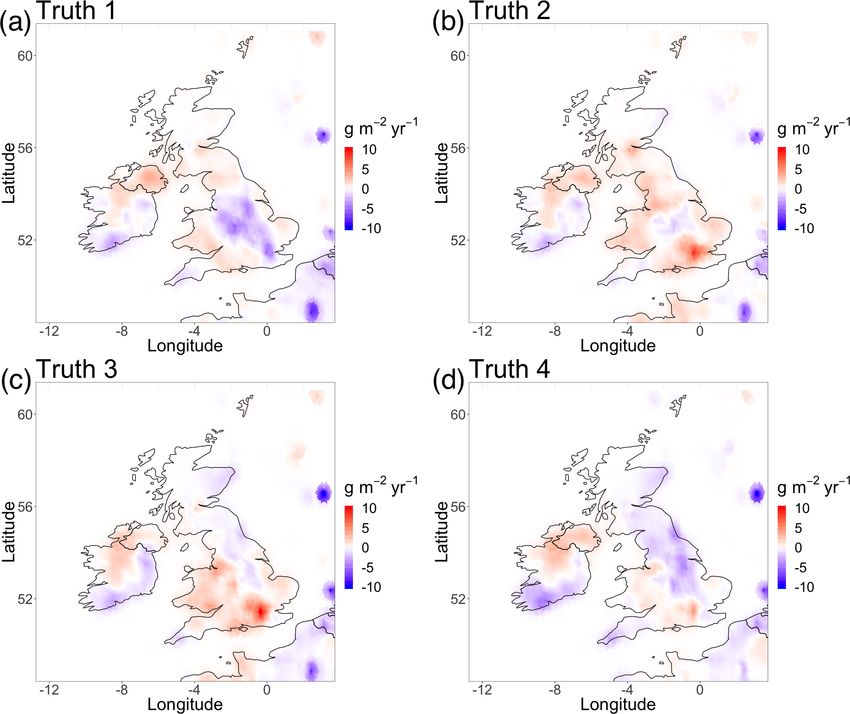
2096                                         L. M. Western et al.: Bayesian spatio-temporal inference of trace gas emissions

posterior solutions that are highly dependent on these as-          2     Methods
sumptions (e.g. Ganesan et al., 2014).
   Recently, hierarchical Bayesian schemes have been devel-         This section details an efficient approach to forming spa-
oped to infer unknown uncertainties in the inversion frame-         tial and spatio-temporal correlation functions and outlines
work (e.g. Ganesan et al., 2014; Jeong et al., 2016; Lunt et al.,   how this applies to the inference of regional trace gas emis-
2016). These hierarchical Bayesian inference schemes use            sions from measurements using fast inference for hierarchi-
Markov chain Monte Carlo (MCMC) methods that are well-              cal models. We limit the scope of this paper to the well-
suited to small-dimensional problems. However, they can             established problem of regional inference of long-lived trace
suffer from issues with convergence, especially as the dimen-       gas emissions using a backward-running Lagrangian particle
sion of the problem increases (Cowles and Carlin, 1996). Hi-        dispersion model (Stohl et al., 2009; Manning et al., 2011;
erarchical inference of spatially and spatio-temporally corre-      Henne et al., 2016). In this framework, the model directly
lated emissions is computationally difficult and currently re-      calculates the sensitivity of the measurements to emissions
lies on methods such as Kalman filters with assumed covari-         from each grid cell in the domain. Extension to other sys-
ance structures (e.g. Brunner et al., 2012) or an empirical hi-     tems (e.g. global models) would require modification to pro-
erarchical framework, where unknown hyperparameters are             vide sensitivity on a global scale with substantially differ-
not integrated out during inference (e.g. Michalak et al.,          ent temporal and spatial emissions. We begin by introducing
2005; Berchet et al., 2015). Previous work shows, however,          the model and the inferred latent parameters (the emission
that including spatial correlation improves the fit between         fluxes and boundary conditions), followed by an introduction
modelled and observed data (Zammit-Mangion et al., 2016),           to Gaussian Markov random fields and how they are useful
while temporal correlation is important to represent the de-        for efficient calculation of spatial and spatio-temporal corre-
pendence of emissions between time periods. The size and            lation structures. All together, this forms a Bayesian hierar-
spatial coverage of measurement networks available for in-          chical model, from which emissions can be inferred.
ferring gas emissions are growing, particularly through satel-
lite observations (e.g. Bergamaschi et al., 2007; Veefkind          2.1    Model framework
et al., 2012; Wecht et al., 2014; Ganesan et al., 2017). There-
                                                                    The aim is to infer some parameters of interest, here a spa-
fore, there is a need to develop methods that can utilise these
                                                                    tial field of a priori emissions scaled by some factor, x, from
big data sets whilst maintaining the benefits of uncertainty
                                                                    some measurement. The a priori emissions at a given loca-
quantification in hierarchical methods, ideally extending to
                                                                    tion are generally informed by spatially resolved bottom-up
spatio-temporal inference.
                                                                    inventories (as in Sect. 3.1.3) or extrapolation from some re-
   This work presents a computationally efficient hierarchi-
                                                                    ported emissions value. The value x is a multiplicative scal-
cal Bayesian framework for inferring spatio-temporally cor-
                                                                    ing of this a priori value for emissions, most generally ex-
related trace gas emissions in a widely used regional atmo-
                                                                    pressed as a quantity of gas per unit time per unit area. The
spheric chemical transport modelling framework. We use an
                                                                    approach taken in this work uses a Gaussian Markov random
integrated nested Laplacian approximation (INLA) for the
                                                                    field for fast and efficient calculation of spatial correlation
Bayesian inference. The spatial correlation structure with
                                                                    for x. This means that the emissions field is required to be
spatial Markov properties results from the Gaussian random
                                                                    a latent Gaussian field, which will be discussed further in
field being a solution to a particular stochastic partial differ-
                                                                    Sect. 2.2. Net surface fluxes of many greenhouse gases are
ential equation. Kronecker product algebra allows efficient
                                                                    positive at the scales resolved by the model. In this work,
extension to spatio-temporal correlation. Section 2 presents
                                                                    due to the usage of a latent Gaussian field, which must be
the construction of the hierarchical problem, describes the
                                                                    defined over both positive and negative values, we choose to
formation of the correlation structure and introduces INLA.
                                                                    look at the deviations of emissions from the prior mean emis-
Section 3 contains two case studies as a proof of concept
                                                                    sions field. This is in an effort to fit the physical model to
for the method with a discussion of their implementation.
                                                                    the imposed statistical model that fast computation requires.
The first is an example using four consecutive periods of
                                                                    Taking the approach that, for many regional inverse problems
pseudo-data observations of methane from four UK moni-
                                                                    involving longer-lived trace gases, there is a linear relation-
toring stations. This then extends to using real observations
                                                                    ship between emissions which are constant in time and ob-
from the four measurement stations to infer UK emissions for
                                                                    served atmospheric concentration, the relationship between
2014, split into four 3-month periods. Section 4 discusses the
                                                                    measurements and emissions is
results and computational performance of the method, and
Sect. 5 presents the conclusions of the study.                      y = Hx + Ku + ,                                           (1)

                                                                    where y is a vector of the residual between the measured and
                                                                    a priori predicted measurement; H is a Jacobian (or sensi-
                                                                    tivity) matrix, which maps the surface emissions to the mea-
                                                                    surements; u is a vector of independent and identically dis-

Geosci. Model Dev., 13, 2095–2107, 2020                                              www.geosci-model-dev.net/13/2095/2020/
L. M. Western et al.: Bayesian spatio-temporal inference of trace gas emissions 2097
tributed variables containing the contribution to the measure-
ment of mole fractions at the boundary of the domain minus
the prior mean contribution, with an associated sensitivity
matrix K; and is some stochastic error. The variable x has
a Gaussian prior probability with zero expectation and a co-
variance described by a Gaussian random field. This will be
solved using a hierarchical framework (Sect. 2.4).
2.2 Gaussian Markov random fields
The emissions scaling from its a priori value x is spatially
continuous over the domain of interest. We assume that it
exhibits a spatial correlation structure because emissions at
one location are generally not independent from all other lo-
cations in the same field. We choose to model the covari-
ance in this field using a Matérn covariance function, which
Stein (1999) shows is well-suited to natural systems due to
Figure 1. A mesh constructed using constrained refined Delaunay
its flexibility, with other correlation structures (e.g. exponen- triangulation, where the distribution of nodes is denser around the
tial) being special cases of the Matérn family (Guttorp and United Kingdom and Ireland.
Gneiting, 2006). A stationary Gaussian random field with a
Matérn covariance is the solution to a particular stochastic
partial differential equation (Whittle, 1954, 1963), given by as the mesh is constructed using Neumann boundary condi-
α
tions, which trigger reflection and therefore overestimation
(κ 2 − 1) 2 (τ x(s)) = W(s), s ∈ , (2) close to the boundaries. This has no effect on the inferred
emissions, provided that the mesh is extended far enough
where κ is the spatial scale parameter, τ influences the vari- around the domain of interest. Figure 1 shows the mesh used
ance, 1 is the Laplacian operator, is the spatial domain and in this work, excluding the extended outer mesh region.
W(s) is a Gaussian stochastic process for locations s, not-
ing that the dependence is only on the Euclidean distance; 2.3 Extension to spatio-temporal correlation
the process is therefore isotropic. For an example of non-
stationary and anisotropic fields see Marques et al. (2019). A spatio-temporal extension to the forward model (Eq. 1) is
The smoothness parameter α gives a continuous domain possible by including the spatial correlation structure intro-
Markov field for integer values and is set to α = 2 (see Whit- duced in Sect. 2.2 in a temporal framework (Cameletti et al.,
tle, 1954). Smaller values will give more short-scale variabil- 2013). Similar to Eq. (1), the deviation from the prior mean
ity and can be difficult to differentiate from noise. Lindgren measurement at site l made at time t in its simplest form is
et al. (2011) show that if the field is represented using a Gaus- n 4
X X
sian Markov random field (see Rue and Held, 2005), then it ytl = hitl xit + kj tl uj t + tl , (4)
is very efficient to directly construct the precision, or inverse i=1 j =1
covariance, matrix using a basis function representation
X where i represents each of the total n nodes and j represents
x(s) = ψk (s)xk , (3) the edge of the domain at each of the four cardinal directions.
k We make the assumption that measurements made at a given
time are independent, giving a vectorised observation vector
where ψk (·) is a piecewise linear function in each triangle of y t at each time. This can be generalised to include correlated
a mesh construction of the spatial domain, where ψk (·) is 1 at measurements, where the covariance function should result
vertex k and 0 at all other vertices. This mesh is created us- in a sparse matrix to retain computational efficiency. Follow-
ing constrained refined Delaunay triangulation (Shewchuk, ing this, the matrix H from Eq. (1) becomes the sparse block
2002), placing nodes at the main points of interests and in- diagonal matrix
filling the rest of the space using some condition of mini-
mum and maximum length of the vertices. In this work we H1 0 0 . . . 0
choose to represent the UK and Ireland with an evenly spaced 0 H2 0 . . . 0
H= . , (5)
denser mesh with a coarser mesh outside of this region. A . .
.. . . .
.. ..
mesh could be further refined, for example by creating an 0 0 0 Hm
even denser mesh close to the measurement site where sen-
sitivity is higher. It is important to extend the mesh beyond which operates on the vectorised spatio-temporal scaling of
the region where the measurements are sensitive to emissions the emissions field x = [x 1 , x 2 , . . .x m ] to model the obser-
www.geosci-model-dev.net/13/2095/2020/ Geosci. Model Dev., 13, 2095–2107, 20202098 L. M. Western et al.: Bayesian spatio-temporal inference of trace gas emissions
vations y = [y 1 , y 2 , . . .y m ]. The time varying structure of Ht We assume
and x applies also to Kt , and ut . We impose the temporal cor-
relation structure between emissions over time to be a first- y | x, u, θ ∼ N (Hx + Ku, Qy (θ )−1 ),
order autoregressive model, where x | u, θ ∼ N (0, Q(θ )−1 ),
2
u | θ ∼ N (0, IσBC ),
x t = φx t−1 + δt ; δt ∼ N 0, Q−1
S t = 1, . . ., m, (6a)
θ ∼ p(θ),
and where the precision matrix of the model–measurement un-
−1 ! certainty Qy contains the hyperparameter for the standard
QS deviation of the model–measurement standard deviation σy ,
x 1 ∼ N 0, , (6b)
1 − φ2 σBC is the standard deviation of the prior for u and I is the
identity matrix. Together the hyperparameters make the vec-
where φ is the temporal correlation and Q−1 tor θ = (ρ, σ, φ, σBC , σy ), which have independent prior dis-
S is the spatial
correlation structure described by a Matérn field using the tributions. The hyperparameters for the spatial precision ma-
stochastic partial differential equation approach for a Gaus- trix Q(θ ) are transformations of the variables in Eq. (2),
sian Markov random field. We have chosen a first-order au- √
8
toregressive model as we believe that emissions are generally ρ= , (9a)
similar to those at the previous time step. In the given model, κ
− 1
φ is the correlation between the previous time step and the 1 2
current time step. This means that the emissions at time t σ= √ , (9b)
4π κτ
have a similarity of φ to emissions at t −1 plus some spatially
correlated random effect δt . The vectorisation of x allows a where ρ is the range parameter and σ is the marginal standard
separable covariance structure for the temporal and spatial deviation of the latent field (Lindgren et al., 2011). We use
covariances, which means that the spatio-temporal precision penalised complexity priors to define the prior probabilities
matrix can be expressed using a Kronecker product as fol- for these parameters (Simpson et al., 2017; Fuglstad et al.,
lows (Mardia et al., 1979): 2018). Penalised complexity priors allow the formation of
priors when there is only a vague understanding of their true
Q = QT ⊗ QS . (7) values while enforcing more constraint than using a broad
uniform or a Jeffreys prior. This uses the information loss of
Estimating hourly emissions at each time t soon makes deviating from some baseline estimate of the parameter. Pe-
inference prohibitive due to burden. Instead we make the as- nalised priors do not increase the computational speed for the
sumption that emissions are constant over a 3-month period given case and are chosen instead for their intuitiveness. Pe-
to reduce the computational size. We continue with the as- nalised complexity priors are specified by the probability of
sumption that measurements within a single time period are the parameters being less than or greater than some baseline
independent, although this can be generalised if required. In value
this experiment we make the assumption that emissions are
constant over a 3-month period and that the correlation be- p(ρ > ρ0 ) = pρ ,
tween these 3-month periods is autoregressive of the order of p(σ < σ0 ) = pσ ,
1.
where ρ0 and σ0 are the baseline values and pρ and pσ are
2.4 Hierarchical model the associated probabilities defined by the user. The hyper-
parameter φ controls the temporal correlation between latent
Inferring the emissions and the related uncertainties requires variables, and its prior probability is defined on a beta distri-
a hierarchical model to infer the quantities of interest from bution scaled between −1 and 1 as
measurements while estimating some unknown parameters
which are necessary for inference. The main focus of this φ ∼ Beta(a, b),
work is to estimate the posterior distribution of the emissions
where a and b are assumed coefficients. The matrix Qy is the
field x based on observations y. We follow a typical Bayesian
precision matrix for the combined measurement and model
hierarchical framework
errors. The diagonal of Qy contains the square of the hyper-
parameter σy , where the prior probability is defined on log σ12
p(x, u, θ | y) ∝ p(y | x, u, θ )p(x | u, θ )p(u | θ )p(θ ), (8) y
as
where θ is vector of hyperparameters describing the vari- 1
log 2 ∼ N µσy , σσ2y .
ances and covariances in x, u and y, noting that x ⊥⊥ y | θ . σy
Geosci. Model Dev., 13, 2095–2107, 2020 www.geosci-model-dev.net/13/2095/2020/L. M. Western et al.: Bayesian spatio-temporal inference of trace gas emissions 2099
The marginal standard deviation of the a priori boundary con- While this method relies on calculating only the marginal
ditions σBC is also constructed this way, giving posterior distributions of xi , it is still possible to predict a
linear combination of the field to provide regional emissions
1
totals (e.g. country totals). We define a linear predictor of
log 2
∼ N µσBC , σσ2BC .
σBC emissions for a given region η∗ , defined using the basis func-
tion representation of the mesh where each node contains in-
A Bayesian hierarchical model requires a method of infer- formation on the spatial area represented by that node and
ence to estimate the parameters of interest and any parame- its connecting vertices and zeros for all nodes that are not in
ters that are not of direct interest but required, and uncertain, the region of interest. Then we can approximate the linear
in order to infer the other parameters in the hierarchy. Many combination of the parameters of interest, giving a combined
methods of inference exist and have been applied to the prob- emissions total η∗ , using Eqs. (11) and (12) and transform-
lem of estimating emissions of trace gases (see references in ing the predicted latent field by the weightings containing the
Sect. 1). A promising approach using the correlation struc- area information.
ture in Sect. 2.2 and 2.3 is INLA (Lindgren and Rue, 2015).
Section 2.5 outlines this approach to inference.
3 Case studies
2.5 Inference using an integrated nested Laplacian
approximation This section presents two case studies to demonstrate how the
method applies to inferring trace gas emissions. The first uses
An integrated nested Laplacian approximation (Rue et al., simulated methane observations from four tall-tower mea-
2009) provides a fast and efficient framework to infer the la- surement sites to infer simulated spatio-temporal emissions
tent variable x and hyperparameters θ from measurements from the UK. The second case study expands on the first case
y. The calculation of the INLA is possible using the R-INLA study by using real observations from the four tall towers to
package (Lindgren and Rue, 2015). In this work we use R- infer emissions of methane from the UK over four 3-month
INLA version 17.06.20. The speed in this approach comes periods in 2014. While the size of this problem is not partic-
from solving the marginal posteriors for xi , i.e. each element ularly large, we demonstrate the method using UK methane
i of the latent field, through the numerical integration emissions as a proof of concept as it is a well-studied test
Z case (Manning et al., 2011; Ganesan et al., 2015; Lunt et al.,
p(θj | y) = p(θ | y)dθ −j , (11) 2015), which should exhibit a spatio-temporal correlation
structure. The method can be extended to larger spatial do-
mains or data set sizes as required.
Z
p(xi | y) = p(xi | y, θ )p(θ | y)dθ , (12) 3.1 Transport model and data
where j is the j th element in θ and −j indicates all by the 3.1.1 Measurement data
element j . Equations (11) and (12) make use of a Laplace
approximation by approximating p(θ | y) by The case study observations are from four measurement
sites: three in the UK and one in Ireland, which are part of the
p(x, θ , y) UK Deriving Emissions related to Climate Change (DECC)
p(θ | y) ∝ , (13)
pG (x | θ , y) x = x ∗ (θ )
network (Stanley et al., 2018). Figure 2 shows the location
of these four measurement stations: Ridge Hill in the west
where pG (x | θ, y) is a Gaussian approximation to the full of England, Angus on the east coast of Scotland, Tacolne-
conditional of x and the right-hand side is evaluated at ston on the east coast of England and Mace Head on the west
x ∗ (θ), which is the modal probability of x for a given coast of Ireland. Measurements are made quasi-continuously
θ . This approximation is exact if p(θ | y) is Gaussian and throughout this network but are averaged into hourly val-
gives a good approximation for log concave problems (Tier- ues here, consistent with the time step of the meteorology
ney and Kadane, 1986). Then, it is possible to approximate that drives the atmospheric transport model (Sect. 3.1.2). The
p(xi | y, θ ) using another Laplace approximation data set contains ∼ 10 000 measurements to demonstrate the
capabilities of the method at handling moderate data vol-
p(x, θ , y) umes. We consider the scalability of this method in the dis-
pLA (xi | θ , y) ∝ , (14)
pG (x −i | xi , θ, y) x −i = x ∗−i (xi ,θ ) cussion (Sect. 4).
where pG (x −i | xi , θ , y) is the Gaussian approximation to 3.1.2 Transport model
x −i | xi , θ , y evaluated at the mode x ∗−i (xi , θ ). See Rue et al.
(2009) and Martins et al. (2013) for a more in-depth descrip- An atmospheric transport model calculates the sensitivity of
tion. hourly measurements to the emissions or boundary condi-
www.geosci-model-dev.net/13/2095/2020/ Geosci. Model Dev., 13, 2095–2107, 20202100 L. M. Western et al.: Bayesian spatio-temporal inference of trace gas emissions
3.2 Pseudo-data experiment
We test the method by performing an inversion using pseudo-
data for four consecutive time periods of 1 month. By cre-
ating a known-emissions field we are able to validate the
method through comparing the inferred emissions to the
known emissions, which is not possible in the real world. We
form a synthetic-emissions field by allowing the emissions to
deviate from the prior mean emissions according to a Matérn
field (see Sect. 2.2). We choose to simulate the data using
σ = 0.5 as the uncertainty in the EDGAR v4.3.2. inventory
is around 50 % for methane emissions and ρ = 3.25, which
is similar to the correlation length scale in UK emissions in
the EDGAR v4.3.2. inventory estimated using a variogram
(Cressie, 2015), although the correlation length scale in the
uncertainty is unknown. We use φ = 0.8 as expert experience
suggests that UK emissions of methane are generally highly
correlated in time.
Figure 2. The case studies use the four UK DECC network mea- To create the synthetic-emissions field, the NAME sen-
surement stations located on this map. RGL is Ridge Hill, TAC is sitivities for each measurement at each grid cell, detailed
Tacolneston, TTA is Angus and MHD is Mace Head station. in Sect. 3.1.1, are multiplied by the corresponding EDGAR
inventory emissions in that grid cell, which are then trans-
formed into the triangulation nodes in Fig. 1. This forms the
tions, from which the matrices H and K can be formed. matrix H. We randomly sample the full spatio-temporal pre-
This work uses the NAME III (Numerical Atmospheric- cision matrix for the latent field (Sect. 2.3) using the GMR-
dispersion Modelling Environment) version 7.2 Lagrangian FLib library (Rue and Follestad, 2001) to generate the latent
particle dispersion model (Jones et al., 2006) to simulate the field x. In this experiment we treat the boundary conditions
transport of methane in the atmosphere. For each measure- as known as in practice these are generally well-constrained
ment, NAME tracks 20 000 gas particles, released over a 1 h (or treated as known) during an inversion. The observations
period, backward in time for 30 d from the measurement site. are simulated using the simulated latent field and sensitivi-
We record the times and locations that the particles drop be- ties following Sect. 2.1 with additive Gaussian noise with a
low 40 m a.g.l. and reach the computational domain bound- standard deviation of 15 % of y. The synthetic observations
ary, which is at 5◦ S, 74◦ N, 55 and 192◦ E, to calculate the contain a total of 11 520 measurement points, which are used
sensitivity of the data to emissions from the surface or to to infer 646 emissions nodes for each time period, i.e. the
the mole fraction at the domain edge. NAME was driven by nodes of the mesh in Fig. 1. Figure 3a–d show the synthetic-
the Met Office’s Unified Model UK Variable (UKV) three- emissions field in terms of deviation from some prior emis-
hourly meteorological analysis (Cullen, 1993). sions field. The synthetic total deviation in emissions from
the prior mean for the UK for each period is 0.07, 1.29, 1.01
3.1.3 Prior emissions inventory and −0.33 Tg yr−1 .
The inference needs prior probabilities for the hyperpa-
Inventory data from the Emissions Database for Global At-
rameters, which are known exactly here, but we set them
mospheric Research (EDGAR) v4.3.2. provide the mean
to be deliberately incorrect, but feasible based on true prior
prior emissions (Janssens-Maenhout et al., 2017) using
knowledge, to check that the inversion method can still re-
the most recent emissions map from 2012. This database
cover the correct emissions. For the inversion we assign a
contains anthropogenic emissions, which are the dominant
prior probability for φ using a = 6.5 and b = 0.1, for σ us-
methane sources in the UK (Manning et al., 2011), and is
ing σ0 = 0.1 and pσ = 0.01 and for ρ using ρ0 = 5 and pρ =
deemed appropriate for the application. The EDGAR emis-
0.5. We base the constraint on the spatio-temporal emissions
sions inventory provides an a priori estimate of UK methane
on the assumption that methane emissions in the UK are
emissions of 2.46 Tg yr−1 . The MOZART-4 global chemistry
likely to be strongly correlated between time periods, that
model (Emmons et al., 2010), driven by global fields of nat-
they are unlikely to vary by more than 10 % of the a priori
ural and anthropogenic emissions and sink terms (Ganesan
emissions from the previous time step and that there is little
et al., 2017), provides the prior mean estimate of methane
knowledge of the spatial correlation structure. For the model
mole fraction at the boundaries of the inversion region.
measurement error we assign the prior probability on the log
precision as log σ12 ∼ N (−5, 1), which represents approxi-
y
Geosci. Model Dev., 13, 2095–2107, 2020 www.geosci-model-dev.net/13/2095/2020/L. M. Western et al.: Bayesian spatio-temporal inference of trace gas emissions 2101
Figure 3. Time-correlated deviation of emissions from the prior mean, simulated using a Matérn field for (a) the first time period, (b) the
second time period, (c) the third time period and (d) the fourth time period.
mately 68 % probability that the error falls between 8 and comparisons of the mean estimates plotted on spatial maps
20 ppb, in line with previous experience. (see Gelman and Price, 1999).
Figure 4 shows the resultant inferred mean changes in the Hyperparameter estimation is less accurate than for the la-
emissions field for each time period using INLA (Sect. 2.5) tent field. The estimation of the noise σy generally captures
and the hierarchical model in Sect. 2.4. The change in the the imposed noise well, which had a mean value of 5.5 ppm
emissions field is the inferred latent field scaling parame- and an estimated value of 6.6 [6.5, 6.8] ppm. The correlation
ter multiplied by the inventory emissions in Sect. 3.1.3. Fig- structures are less well-captured. The temporal correlation φ
ure S1 shows maps of the 95 % uncertainty in the difference was estimated with a mean value of 0.7 [0.6, 0.8]; the range
in emissions. A linear combination of the posterior latent ρ has a value of 1.7 [1.3, 2.1] and the marginal standard de-
field multiplied by the inventory emissions field gives total viation of the latent field σ has a value of 0.8 [0.7,0.9]. It is
emissions for the UK. The inferred posterior mean change in promising that the posterior mean estimates of all hyperpa-
total emissions for the UK from the prior mean with their as- rameters show an improvement on their prior mean or base-
sociated 95 % uncertainties for the four time periods are 0.01 line values, although only the true value for ρ falls within the
[−0.10, 0.12], 1.23 [1.10, 1.36], 1.07 [0.97, 1.18] and −0.30 estimated 95 % uncertainty.
[−0.41, −0.18] Tg yr−1 , which are shown in Fig. 5. The in-
ferred emissions for the UK as a whole agree well with the 3.3 Real-data experiment
synthetic emissions, with all true synthetic emissions totals
falling within the 95 % uncertainty of the inferred total emis- This section presents methane emissions estimates for the
sions. These synthetic tests cover both small and large differ- UK in 2014. The year is split into four time periods: Jan-
ences between the a priori estimate of methane emissions in uary to March, April to June, July to September and October
the UK and their true value. The larger differences are most to December. Based on the synthetic data set in Sect. 3.2, we
likely an overestimate of what would be expected in practice, use the same prior probabilities for the hyperparameters as
although this provides a good test case. The posterior mean the inversion. The prior boundary conditions are distributed
spatial distribution of emissions in Fig. 4 is qualitatively sim- with µσBC = 3.2 and σσBC = 0.4, based on expert judgement.
ilar to those in Fig. 3, although we avoid reading heavily into The a priori values for these boundary conditions come from
the MOZART-4 model as in Sect. 3.1.3. The linear mapping
www.geosci-model-dev.net/13/2095/2020/ Geosci. Model Dev., 13, 2095–2107, 20202102 L. M. Western et al.: Bayesian spatio-temporal inference of trace gas emissions
Figure 4. The inferred mean deviation of emissions from the prior mean for (a) the first time period, (b) the second time period, (c) the third
time period and (d) the fourth time period.
Figure 6 shows maps of the inferred mean difference in
emissions from the a priori inventory for the four time peri-
ods using INLA as in Sect. 2.5. This result is the mean pos-
terior scaling for the latent field multiplied by the inventory
value (see Sect. 3.1.3). Figure S2 shows maps of the 95 %
uncertainty in the difference in emissions. A linear combi-
nation of the posterior latent field multiplied by the inven-
tory emissions field gives total emissions for the UK. We
estimate total UK methane emissions in 2014, with their as-
sociated 95 % uncertainty, of 2.14 [1.90, 2.38], 2.28 [2.06,
2.51], 2.62 [2.39, 2.84] and 2.09 [1.87, 2.30] Tg yr−1 for the
periods January to March, April to June, July to Septem-
ber and October to December, respectively. These are plot-
ted along with the inventory estimate in Fig. 7. This emis-
sions trend suggests that, for 2014, there was an increase
Figure 5. The inferred and true difference between UK emissions in methane emissions in the UK during the summer months
and a synthetic inventory value for each of the four time periods. compared to the winter months. The uncertainties, however,
The crosses show the inferred mean difference in total emissions are large, meaning that this increase may not be as stark as
with their associated 95 % uncertainty. The red line indicates one- suggested by the mean estimates. Combining these emissions
to-one agreement. into a mean annual emission for 2014 with its associated 2-
standard-deviation uncertainty assuming that the time peri-
ods are correlated with the modal posterior value of φ gives
from the latent field to the measurements is generated using 2.28 ± 0.33 Tg yr−1 . The emissions are similar to mean UK
the NAME-derived sensitivities described in Sect. 3.1.2 mul- estimates from previous hierarchical inversions using NAME
tiplied by the inventory emissions detailed in Sect. 3.1.3. of 2.09 [1.65, 2.67] Tg yr−1 by Ganesan et al. (2015) and
2.28 [2.04, 2.52] Tg yr−1 by Lunt et al. (2016). All of these
Geosci. Model Dev., 13, 2095–2107, 2020 www.geosci-model-dev.net/13/2095/2020/L. M. Western et al.: Bayesian spatio-temporal inference of trace gas emissions 2103
Figure 6. Inferred mean difference in methane emissions for the UK in 2014 compared to the EDGAR inventory for (a) January to March,
(b) April to June, (c) July to September and (d) October to December.
estimates are broadly in line with the United Kingdom’s 2014
emissions estimate of 2.13 Tg yr−1 reported in its national
inventory (Department of Business, Energy and Industrial
Strategy, 2019).
4 Discussion
The real benefit of the presented inversion method is speed,
while still maintaining the idea that, in this application, un-
certainties exist within the uncertainties that are inherent to
hierarchical Bayesian inverse methods. The computation of
the marginal posterior distribution of the latent field is read-
ily suited to run in parallel across multiple cores, making this
approach scalable to problems with a larger parameter space.
This, however, requires that sufficient memory allocation is
available. The inference for the experiment in Sect. 3.3 took
around 2 h wall-clock time using a Quad-Core MacBook Pro Figure 7. Estimated total UK methane emissions for 2014. The
with 8 GB RAM. For comparison, we were unable to get the prior mean comes from EDGAR v4.32 inventory data (red dashed).
problem in Sect. 3.3 to converge using 22 million iterations For comparison, the figure also shows the posterior means for UK
of a Metropolis-adjusted Langevin diffusion MCMC algo- methane emissions from Ganesan et al. (2015) (black dotted) and
Lunt et al. (2016) (black dash-dotted).
rithm (Roberts and Rosenthal, 1998), taking on the order of
days to complete and whose convergence is difficult to di-
agnose (Cowles and Carlin, 1996). Reducing the problem to
purely spatial inference reduces the run time down to around hierarchical methods other than MCMC, for example empir-
10 min wall-clock time for a single 3-month period. Infer- ical hierarchical inference (e.g. Michalak et al., 2005). Such
ence using INLA may have smaller computational gains over methods, however, would benefit from using the stochastic
www.geosci-model-dev.net/13/2095/2020/ Geosci. Model Dev., 13, 2095–2107, 20202104 L. M. Western et al.: Bayesian spatio-temporal inference of trace gas emissions
partial differential equation approach to Gaussian Markov 5 Conclusions
random fields for spatial correlation in Sect. 2.2, vastly re-
ducing the cost of inverting dense covariance matrices.
The latent Gaussian field, crucial to this method, has the This work presents a fast and efficient method using an inte-
problem that it does not restrict emissions to strictly positive grated nested Laplacian approximation for hierarchical infer-
values, which is a physical requirement for many gas emis- ence of trace gas emissions. This method is particularly well-
sions. In addition, the INLA method relies on the assump- suited to assimilating large data sets. We show that INLA
tion of approximate multivariate normality of the posterior with a stochastic partial differential equation approach for
linear predictors. MCMC algorithms do not suffer from this spatial correlation can reproduce synthetic emissions from
issue as any prior probability density function can be chosen, pseudo-observations and benchmarked emissions using real
data.
and no assumption is made about the posterior linear predic-
tors. This has to be traded off, however, with the speed and A real advantage over other hierarchical Bayesian inver-
ease of implementation of the method and the scale of the sion methods is the attractive convergence properties, which
problem that the user wishes to solve. If strictly positive pos- can be difficult to obtain using methods such as Markov
terior emissions are an absolute requirement, another possi- chain Monte Carlo algorithms. As the method computes the
ble modification to the approach is to use a Taylor expansion marginal variance for each node, this allows for efficient
around the nonlinear model Z = Hex + , where x is a mul- parallel implementation and significant computational sav-
tiplicative scaling of the prior mode which follows a Matérn ings compared to other hierarchical methods. Computational
field. This Taylor expansion could either be around zero if speed will become increasingly important as more data from
the prior inventory is a good estimate of the true emissions or space-borne sensors become available, which will offer more
around the posterior mode itself, which can be found through measurements and increased spatial coverage.
iterations of the inverse method at the posterior mode of the
previous iteration. An alternative route would be to instead
Code and data availability. Measurements of methane from the
use a non-Gaussian Matérn field, and this will likely prove a UK DECC network sites Tacolneston, Ridge Hill and Tall Tower
promising future avenue for geostatistical inference (Wallin Angus are available at http://ebas.nilu.no/ (last access: 13 Febru-
and Bolin, 2015). ary 2020, Tørseth et al., 2012). Measurements of methane for the
A potential extension to this work is global-scale mod- Mace Head station are available at http://agage.mit.edu/data (last
elling, for example a global study of methane emission from access: 13 February 2020, Prinn et al., 2020). The NAME III
global satellite measurements. Spatio-temporal estimation of v7.2 transport model is available from the UK Met Office un-
global CO2 fluxes using Gaussian Markov random fields der licence by contacting enquiries@metoffice.gov.uk. The mete-
and a global measurement network gives promising results orological data used in this work from the UK Met Office opera-
(Dahlén et al., 2019). The nature of the method makes it tional NWP (Numerical Weather Prediction) Unified Model (UM)
well-suited to parallel implementation and thus upscaling. are available from the UK Centre for Environmental Data Analy-
sis at http://data.ceda.ac.uk/badc/ukmo-nwp (last access: 13 Febru-
Upscaling to global studies may introduce additional diffi-
ary 2020, Met Office, 2013). The MOZART-4 global chemistry
culties, which have been otherwise ignored in the regional model is available at https://www2.acom.ucar.edu/gcm/mozart-4
case. For example it may no longer be possible to assume a (last access: 13 February 2020, Emmons et al., 2010). The R-
spatial correlation structure controlled by only two hyperpa- INLA v17.06.20 library is available for download from http://www.
rameters, i.e. the correlation structure may vary in space. The r-inla.org/download (last access: 13 February 2020, Lindgren and
stochastic partial differential equation approach to Gaussian Rue, 2015), which includes the GMRFLib library. The EDGAR
Markov random fields can handle this by allowing the hyper- v.4.3.2 methane inventory can be downloaded from https://edgar.
parameters ρ and σ to become vectors or a non-stationary jrc.ec.europa.eu/overview.php?v=432_GHG (last access: 13 Febru-
covariance (Lindgren et al., 2011) or by subsetting the space ary 2020, Janssens-Maenhout et al., 2017). The code and data
controlled by the different covariance structures (Sha et al., to infer emissions using the simulated data in Sect. 3.2 can be
2019). The problem of non-stationary covariances may also found at https://osf.io/53w96 (last access: 13 February 2020) and
https://doi.org/10.17605/OSF.IO/53W96 (Western, 2019). Any fur-
be present for inference of other spatial scales. For exam-
ther data or code is available from the corresponding author on re-
ple natural features, such as lakes, may cause abrupt changes quest.
in correlation structures. Emissions of anthropogenic green-
house gases may exhibit no spatial correlation structure (e.g.
Mühle et al., 2019; Rigby et al., 2019). In this case a Matérn Supplement. The supplement related to this article is available on-
field would be inappropriate, but an autoregressive model line at: https://doi.org/10.5194/gmd-13-2095-2020-supplement.
may still be applicable for time-varying emissions. The in-
clusion of a non-stationary covariance makes the problem
much more computationally expensive, and a more parsimo- Author contributions. LW and ZS conceived and led the implemen-
nious approach may often suffice (Fuglstad et al., 2015). tation of the study. MR, AG and JR supported and advised on the
study. KS, SO and DY made the measurements from the UK DECC
Geosci. Model Dev., 13, 2095–2107, 2020 www.geosci-model-dev.net/13/2095/2020/L. M. Western et al.: Bayesian spatio-temporal inference of trace gas emissions 2105
network. AM created the sensitivity footprints using the NAME Phys., 17, 10651–10674, https://doi.org/10.5194/acp-17-10651-
model. LW led the writing of the manuscript, to which all authors 2017, 2017.
have contributed and edited. Cameletti, M., Lindgren, F., Simpson, D., and Rue, H.: Spatio-
temporal modeling of particulate matter concentration through
the SPDE approach, ASTA-Adv. Stat. Anal., 97, 109–131,
Competing interests. The authors declare that they have no conflict https://doi.org/10.1007/s10182-012-0196-3, 2013.
of interest. Cowles, M. K. and Carlin, B. P.: Markov Chain Monte Carlo Con-
vergence Diagnostics: A Comparative Review, J. Am. Stat. As-
soc., 91, 883–904, https://doi.org/10.2307/2291683, 1996.
Acknowledgements. We would like to thank Alfredo Farjat and an Cressie, N. A. C.: Statistics for spatial data, John Wiley & Sons,
anonymous reviewer for their helpful reviews of the manuscript. Inc, Hoboken, NJ, revised edition, 2015.
Cullen, M. J. P.: The Unified Forecast/Climate Model, Meteorol.
Mag., 122, 81–94, 1993.
Dahlén, U., Lindström, J., and Scholze, M.: Spatiotempo-
Financial support. This work was funded by the Jean Golding In-
ral reconstructions of global CO2 -fluxes using Gaus-
stitute Seed Corn grant CHEM.HF8064. Luke Western was funded
sian Markov random fields, Environmetrics, 2019, e2610,
by grants NE/M014851/1 and NE/S016155/1 from the Natural En-
https://doi.org/10.1002/env.2610, 2019.
vironment Research Council and a grant from the UK Department
Department of Business, Energy and Industrial Strategy: 2017 UK
for Business, Energy and Industrial Strategy. Anita Ganesan was
Greenhouse Gas Emissions, Final Figures, 2019.
funded under a Natural Environment Research Council Independent
Emmons, L. K., Walters, S., Hess, P. G., Lamarque, J.-F., Pfis-
Research Fellowship NE/L010992/1.
ter, G. G., Fillmore, D., Granier, C., Guenther, A., Kinnison,
D., Laepple, T., Orlando, J., Tie, X., Tyndall, G., Wiedinmyer,
C., Baughcum, S. L., and Kloster, S.: Description and eval-
Review statement. This paper was edited by Ignacio Pisso and re- uation of the Model for Ozone and Related chemical Trac-
viewed by Alfredo Farjat and one anonymous referee. ers, version 4 (MOZART-4), Geosci. Model Dev., 3, 43–67,
https://doi.org/10.5194/gmd-3-43-2010, 2010.
Fuglstad, G.-A., Simpson, D., Lindgren, F., and Rue, H.:
Does non-stationary spatial data always require non-
stationary random fields?, Spat. Stat., 14, 505–531,
References https://doi.org/10.1016/j.spasta.2015.10.001, 2015.
Fuglstad, G.-A., Simpson, D., Lindgren, F., and Rue, H.:
Berchet, A., Pison, I., Chevallier, F., Bousquet, P., Bonne, J.-L., Constructing Priors that Penalize the Complexity of Gaus-
and Paris, J.-D.: Objectified quantification of uncertainties in sian Random Fields, J. Am. Stat. Assoc., 114, 445–452,
Bayesian atmospheric inversions, Geosci. Model Dev., 8, 1525– https://doi.org/10.1080/01621459.2017.1415907, 2018.
1546, https://doi.org/10.5194/gmd-8-1525-2015, 2015. Ganesan, A. L., Rigby, M., Zammit-Mangion, A., Manning, A. J.,
Bergamaschi, P., Frankenberg, C., Meirink, J. F., Krol, M., Prinn, R. G., Fraser, P. J., Harth, C. M., Kim, K.-R., Krummel,
Dentener, F., Wagner, T., Platt, U., Kaplan, J. O., Körner, P. B., Li, S., Mühle, J., O’Doherty, S. J., Park, S., Salameh,
S., Heimann, M., Dlugokencky, E. J., and Goede, A.: P. K., Steele, L. P., and Weiss, R. F.: Characterization of un-
Satellite chartography of atmospheric methane from SCIA- certainties in atmospheric trace gas inversions using hierarchi-
MACHY on board ENVISAT: 2. Evaluation based on inverse cal Bayesian methods, Atmos. Chem. Phys., 14, 3855–3864,
model simulations, J. Geophys. Res.-Atmos., D02304, 112, https://doi.org/10.5194/acp-14-3855-2014, 2014.
https://doi.org/10.1029/2006JD007268, 2007. Ganesan, A. L., Manning, A. J., Grant, A., Young, D., Oram,
Brioude, J., Angevine, W. M., Ahmadov, R., Kim, S.-W., Evan, S., D. E., Sturges, W. T., Moncrieff, J. B., and O’Doherty, S.:
McKeen, S. A., Hsie, E.-Y., Frost, G. J., Neuman, J. A., Pol- Quantifying methane and nitrous oxide emissions from the UK
lack, I. B., Peischl, J., Ryerson, T. B., Holloway, J., Brown, and Ireland using a national-scale monitoring network, Atmos.
S. S., Nowak, J. B., Roberts, J. M., Wofsy, S. C., Santoni, G. Chem. Phys., 15, 6393–6406, https://doi.org/10.5194/acp-15-
W., Oda, T., and Trainer, M.: Top-down estimate of surface flux 6393-2015, 2015.
in the Los Angeles Basin using a mesoscale inverse modeling Ganesan, A. L., Rigby, M., Lunt, M. F., Parker, R. J., Boesch,
technique: assessing anthropogenic emissions of CO, NOx and H., Goulding, N., Umezawa, T., Zahn, A., Chatterjee, A., Prinn,
CO2 and their impacts, Atmos. Chem. Phys., 13, 3661–3677, R. G., Tiwari, Y. K., van der Schoot, M., and Krummel, P. B.:
https://doi.org/10.5194/acp-13-3661-2013, 2013. Atmospheric observations show accurate reporting and little
Brunner, D., Henne, S., Keller, C. A., Reimann, S., Vollmer, M. growth in India’s methane emissions, Nat. Commun., 8, 836,
K., O’Doherty, S., and Maione, M.: An extended Kalman- https://doi.org/10.1038/s41467-017-00994-7, 2017.
filter for regional scale inverse emission estimation, Atmos. Gelman, A. and Price, P. N.: All maps of param-
Chem. Phys., 12, 3455–3478, https://doi.org/10.5194/acp-12- eter estimates are misleading, Stat. Med., 18,
3455-2012, 2012. 3221–3234, https://doi.org/10.1002/(SICI)1097-
Brunner, D., Arnold, T., Henne, S., Manning, A., Thompson, R. 0258(19991215)18:233.0.CO;2-M,
L., Maione, M., O’Doherty, S., and Reimann, S.: Comparison of 1999.
four inverse modelling systems applied to the estimation of HFC-
125, HFC-134a, and SF6 emissions over Europe, Atmos. Chem.
www.geosci-model-dev.net/13/2095/2020/ Geosci. Model Dev., 13, 2095–2107, 20202106 L. M. Western et al.: Bayesian spatio-temporal inference of trace gas emissions Guttorp, P. and Gneiting, T.: Studies in the history of probability and Mardia, K. V., Kent, J. T., and Bibby, J. M.: Multivariate analysis, statistics XLIX On the Matérn correlation family, Biometrika, Probability and mathematical statistics, Academic Press, Lon- 93, 989–995, https://doi.org/10.1093/biomet/93.4.989, 2006. don, New York, 1979. Henne, S., Brunner, D., Oney, B., Leuenberger, M., Eugster, W., Marques, I., Klein, N., and Kneib, T.: Non-stationary spatial regres- Bamberger, I., Meinhardt, F., Steinbacher, M., and Emmeneg- sion for modelling monthly precipitation in Germany, Spat. Stat., ger, L.: Validation of the Swiss methane emission inventory 100386, https://doi.org/10.1016/j.spasta.2019.100386, 2019. by atmospheric observations and inverse modelling, Atmos. Martins, T. G., Simpson, D., Lindgren, F., and Rue, H.: Bayesian Chem. Phys., 16, 3683–3710, https://doi.org/10.5194/acp-16- computing with INLA: New features, Comput. Stat. Data An., 3683-2016, 2016. 67, 68–83, https://doi.org/10.1016/j.csda.2013.04.014, 2013. Janssens-Maenhout, G., Crippa, M., Guizzardi, D., Muntean, M., Met Office: Operational Numerical Weather Prediction (NWP) Schaaf, E., Dentener, F., Bergamaschi, P., and Pagliari, V.: Output from the UK Variable (UKV) Resolution Part of EDGAR v4.3.2 Global Atlas of the three major Greenhouse Gas the Met Office Unified Model (UM), NCAS British At- Emissions for the period 1970-2012, Open Access, p. 55, 2017. mospheric Data Centre, available at: http://catalogue.ceda. Jeong, S., Newman, S., Zhang, J., Andrews, A. E., Bianco, L., ac.uk/uuid/292da1ccfebd650f6d123e53270016a8 (last access: Bagley, J., Cui, X., Graven, H., Kim, J., Salameh, P., LaFranchi, 13 February 2020), 2013 B. W., Priest, C., Campos-Pineda, M., Novakovskaia, E., Sloop, Michalak, A. M., Hirsch, A., Bruhwiler, L., Gurney, K. R., Pe- C. D., Michelsen, H. A., Bambha, R. P., Weiss, R. F., Keeling, ters, W., and Tans, P. P.: Maximum likelihood estimation of R., and Fischer, M. L.: Estimating methane emissions in Cali- covariance parameters for Bayesian atmospheric trace gas sur- fornia’s urban and rural regions using multitower observations: face flux inversions, J. Geophys. Res.-Atmos., 110, D24107, Methane Emissions in California, J. Geophys. Res.-Atmos., 121, https://doi.org/10.1029/2005JD005970, 2005. 13031–13049, https://doi.org/10.1002/2016JD025404, 2016. Mühle, J., Trudinger, C. M., Western, L. M., Rigby, M., Vollmer, Jones, A., Thomson, D., Hort, M., and Devenish, B.: The U.K. M. K., Park, S., Manning, A. J., Say, D., Ganesan, A., Steele, Met Office’s Next-Generation Atmospheric Dispersion Model, L. P., Ivy, D. J., Arnold, T., Li, S., Stohl, A., Harth, C. M., NAME III, in: Air Pollution Modeling and Its Application XVII, Salameh, P. K., McCulloch, A., O’Doherty, S., Park, M.-K., Jo, edited by Borrego, C. and Norman, A.-L., Springer US, Boston, C. O., Young, D., Stanley, K. M., Krummel, P. B., Mitrevski, MA, 580–589, https://doi.org/10.1007/978-0-387-68854-1_62, B., Hermansen, O., Lunder, C., Evangeliou, N., Yao, B., Kim, J., 2006. Hmiel, B., Buizert, C., Petrenko, V. V., Arduini, J., Maione, M., Leip, A., Skiba, U., Vermeulen, A., and Thompson, R. L.: A com- Etheridge, D. M., Michalopoulou, E., Czerniak, M., Severing- plete rethink is needed on how greenhouse gas emissions are haus, J. P., Reimann, S., Simmonds, P. G., Fraser, P. J., Prinn, R. quantified for national reporting, Atmos. Environ., 174, 237–240, G., and Weiss, R. F.: Perfluorocyclobutane (PFC-318, c-C4F8) in https://doi.org/10.1016/j.atmosenv.2017.12.006, 2018. the global atmosphere, Atmos. Chem. Phys., 19, 10335–10359, Lindgren, F. and Rue, H.: Bayesian Spatial Modelling with R - https://doi.org/10.5194/acp-19-10335-2019, 2019. INLA, J. Stat. Softw., 63, https://doi.org/10.18637/jss.v063.i19, Prinn, R. G., Weiss, R. F., Arduini, J., Arnold, T., Fraser, P. J., 2015. Ganesan, A. L., Gasore, J., Harth, C. M., Hermansen, O., Kim, Lindgren, F., Rue, H., and Lindström, J.: An explicit link between J., Krummel, P. B., Li, S., Loh, Z. M., Lunder, C. R., Maione, Gaussian fields and Gaussian Markov random fields: the stochas- M., Manning, A. J., Miller, B. R., Mitrevski, B., Mühle, J., tic partial differential equation approach: Link between Gaussian O’Doherty, S., Park, S., Reimann, S., Rigby, M., Salameh, P. Fields and Gaussian Markov Random Fields, J. Roy. Stat. Soc. B, K., Schmidt, R., Simmonds, P.G., Steele, L. P., Vollmer, M. 73, 423–498, https://doi.org/10.1111/j.1467-9868.2011.00777.x, K., Wang, R. H., and Young, D.: The ALE/GAGE/AGAGE 2011. Data Base, available at: http://agage.mit.edu/data, last access: Lunt, M. F., Rigby, M., Ganesan, A. L., Manning, A. J., Prinn, 13 February 2020. R. G., O’Doherty, S., Mühle, J., Harth, C. M., Salameh, P. K., Rigby, M., Park, S., Saito, T., Western, L. M., Redington, A. L., Arnold, T., Weiss, R. F., Saito, T., Yokouchi, Y., Krummel, Fang, X., Henne, S., Manning, A. J., Prinn, R. G., Dutton, G. S., P. B., Steele, L. P., Fraser, P. J., Li, S., Park, S., Reimann, S., Fraser, P. J., Ganesan, A. L., Hall, B. D., Harth, C. M., Kim, Vollmer, M. K., Lunder, C., Hermansen, O., Schmidbauer, N., J., Kim, K.-R., Krummel, P. B., Lee, T., Li, S., Liang, Q., Lunt, Maione, M., Arduini, J., Young, D., and Simmonds, P. G.: Rec- M. F., Montzka, S. A., Mühle, J., O’Doherty, S., Park, M.-K., onciling reported and unreported HFC emissions with atmo- Reimann, S., Salameh, P. K., Simmonds, P., Tunnicliffe, R. L., spheric observations, P. Natl. Acad. Sci. USA, 112, 5927–5931, Weiss, R. F., Yokouchi, Y., and Young, D.: Increase in CFC- https://doi.org/10.1073/pnas.1420247112, 2015. 11 emissions from eastern China based on atmospheric obser- Lunt, M. F., Rigby, M., Ganesan, A. L., and Manning, A. J.: Esti- vations, Nature, 569, 546–550, https://doi.org/10.1038/s41586- mation of trace gas fluxes with objectively determined basis func- 019-1193-4, 2019. tions using reversible-jump Markov chain Monte Carlo, Geosci. Roberts, G. O. and Rosenthal, J. S.: Optimal scaling of discrete ap- Model Dev., 9, 3213–3229, https://doi.org/10.5194/gmd-9-3213- proximations to Langevin diffusions, J. Roy. Stat. Soc. B, 60, 2016, 2016. 255–268, https://doi.org/10.1111/1467-9868.00123, 1998. Manning, A. J., O’Doherty, S., Jones, A. R., Simmonds, Rue, H. and Follestad, T.: GMRFLib: a C-library for fast and exact P. G., and Derwent, R. G.: Estimating UK methane and ni- simulation of Gaussian Markov random fields, Tech. rep., SIS- trous oxide emissions from 1990 to 2007 using an inver- 2002-236, 2001. sion modeling approach, J. Geophys. Res., 116, D02305, https://doi.org/10.1029/2010JD014763, 2011. Geosci. Model Dev., 13, 2095–2107, 2020 www.geosci-model-dev.net/13/2095/2020/
L. M. Western et al.: Bayesian spatio-temporal inference of trace gas emissions                                                            2107

Rue, H. and Held, L.: Gaussian Markov random fields: theory                Tierney, L. and Kadane, J. B.: Accurate Approximations for Poste-
   and applications, Chapman & Hall/CRC, Boca Raton, oCLC:                    rior Moments and Marginal Densities, J. Am. Stat. Assoc., 81,
   839047556, 2005.                                                           82–86, https://doi.org/10.2307/2287970, 1986.
Rue, H., Martino, S., and Chopin, N.: Approximate Bayesian in-             Tørseth, K., Aas, W., Breivik, K., Fjæraa, A. M., Fiebig, M.,
   ference for latent Gaussian models by using integrated nested              Hjellbrekke, A. G., Lund Myhre, C., Solberg, S., and Yttri,
   Laplace approximations, J. Roy. Stat. Soc. B, 71, 319–392,                 K. E.: Introduction to the European Monitoring and Evalua-
   https://doi.org/10.1111/j.1467-9868.2008.00700.x, 2009.                    tion Programme (EMEP) and observed atmospheric composition
Saunois, M., Bousquet, P., Poulter, B., Peregon, A., Ciais, P.,               change during 1972–2009, Atmos. Chem. Phys., 12, 5447–5481,
   Canadell, J. G., Dlugokencky, E. J., Etiope, G., Bastviken, D.,            https://doi.org/10.5194/acp-12-5447-2012, 2012.
   Houweling, S., Janssens-Maenhout, G., Tubiello, F. N., Castaldi,        Veefkind, J., Aben, I., McMullan, K., Förster, H., de Vries,
   S., Jackson, R. B., Alexe, M., Arora, V. K., Beerling, D. J., Berga-       J., Otter, G., Claas, J., Eskes, H., de Haan, J., Kleipool,
   maschi, P., Blake, D. R., Brailsford, G., Brovkin, V., Bruhwiler,          Q., van Weele, M., Hasekamp, O., Hoogeveen, R., Landgraf,
   L., Crevoisier, C., Crill, P., Covey, K., Curry, C., Frankenberg, C.,      J., Snel, R., Tol, P., Ingmann, P., Voors, R., Kruizinga, B.,
   Gedney, N., Höglund-Isaksson, L., Ishizawa, M., Ito, A., Joos, F.,         Vink, R., Visser, H., and Levelt, P.: TROPOMI on the ESA
   Kim, H.-S., Kleinen, T., Krummel, P., Lamarque, J.-F., Langen-             Sentinel-5 Precursor: A GMES mission for global observations
   felds, R., Locatelli, R., Machida, T., Maksyutov, S., McDonald,            of the atmospheric composition for climate, air quality and
   K. C., Marshall, J., Melton, J. R., Morino, I., Naik, V., O’Doherty,       ozone layer applications, Remote Sens. Environ., 120, 70–83,
   S., Parmentier, F.-J. W., Patra, P. K., Peng, C., Peng, S., Peters,        https://doi.org/10.1016/j.rse.2011.09.027, 2012.
   G. P., Pison, I., Prigent, C., Prinn, R., Ramonet, M., Riley, W.        Wallin, J. and Bolin, D.: Geostatistical Modelling Using Non-
   J., Saito, M., Santini, M., Schroeder, R., Simpson, I. J., Spahni,         Gaussian Matérn Fields, Scand. J. Stat., 42, 872–890,
   R., Steele, P., Takizawa, A., Thornton, B. F., Tian, H., Tohjima,          https://doi.org/10.1111/sjos.12141, 2015.
   Y., Viovy, N., Voulgarakis, A., van Weele, M., van der Werf, G.         Wecht, K. J., Jacob, D. J., Sulprizio, M. P., Santoni, G. W., Wofsy,
   R., Weiss, R., Wiedinmyer, C., Wilton, D. J., Wiltshire, A., Wor-          S. C., Parker, R., Bösch, H., and Worden, J.: Spatially resolv-
   thy, D., Wunch, D., Xu, X., Yoshida, Y., Zhang, B., Zhang, Z.,             ing methane emissions in California: constraints from the Cal-
   and Zhu, Q.: The global methane budget 2000–2012, Earth Syst.              Nex aircraft campaign and from present (GOSAT, TES) and fu-
   Sci. Data, 8, 697–751, https://doi.org/10.5194/essd-8-697-2016,            ture (TROPOMI, geostationary) satellite observations, Atmos.
   2016.                                                                      Chem. Phys., 14, 8173–8184, https://doi.org/10.5194/acp-14-
Sha, Z., Rougier, J. C., Schumacher, M., and Bamber, J. L.:                   8173-2014, 2014.
   Bayesian model–data synthesis with an application to                    Western,            L.:          INLA_GHG_GMD,                  OSF,
   global glacio-isostatic adjustment, Environmetrics, 30, e2530,             https://doi.org/10.17605/OSF.IO/53W96, 2019.
   https://doi.org/10.1002/env.2530, 2019.                                 Whittle, P.: On Stationary Processes in the Plane, Biometrika, 434–
Shewchuk, J. R.: Delaunay refinement algorithms for tri-                      449, 1954.
   angular mesh generation, Comp. Geom., 22, 21–74,                        Whittle, P.: Stochastic-processes in several dimensions, Int Statisti-
   https://doi.org/10.1016/S0925-7721(01)00047-5, 2002.                       cal Institude 428 Prinses Beatrixlaen, Voorburg, the Netherlands,
Simpson, D., Rue, H., Riebler, A., Martins, T. G., and Sørbye,                40, 974–994, 1963.
   S. H.: Penalising Model Component Complexity: A Principled,             Zammit-Mangion, A., Cressie, N., and Ganesan, A. L.:
   Practical Approach to Constructing Priors, Stat. Sci., 32, 1–28,           Non-Gaussian bivariate modelling with application to at-
   https://doi.org/10.1214/16-STS576, 2017.                                   mospheric trace-gas inversion, Spat. Stat., 18, 194–220,
Stanley, K. M., Grant, A., O’Doherty, S., Young, D., Manning, A.              https://doi.org/10.1016/j.spasta.2016.06.005, 2016.
   J., Stavert, A. R., Spain, T. G., Salameh, P. K., Harth, C. M., Sim-
   monds, P. G., Sturges, W. T., Oram, D. E., and Derwent, R. G.:
   Greenhouse gas measurements from a UK network of tall towers:
   technical description and first results, Atmos. Meas. Tech., 11,
   1437–1458, https://doi.org/10.5194/amt-11-1437-2018, 2018.
Stein, M. L.: Interpolation of Spatial Data: Some Theory for Krig-
   ing, Springer Series in Statistics, Springer, New York, 1999.
Stohl, A., Seibert, P., Arduini, J., Eckhardt, S., Fraser, P., Gre-
   ally, B. R., Lunder, C., Maione, M., Mühle, J., O’Doherty, S.,
   Prinn, R. G., Reimann, S., Saito, T., Schmidbauer, N., Sim-
   monds, P. G., Vollmer, M. K., Weiss, R. F., and Yokouchi, Y.:
   An analytical inversion method for determining regional and
   global emissions of greenhouse gases: Sensitivity studies and
   application to halocarbons, Atmos. Chem. Phys., 9, 1597–1620,
   https://doi.org/10.5194/acp-9-1597-2009, 2009.

www.geosci-model-dev.net/13/2095/2020/                                                         Geosci. Model Dev., 13, 2095–2107, 2020
You can also read