Technical Report on Aircraft Emissions Inventory and Stringency Analysis - EPA

Technical Report on Aircraft Emissions
 Inventory and Stringency Analysis

 July 2020

 US EPA Office of Transportation and Air Quality
 Assessment and Standards Division

 Disclaimer

 This technical report does not necessarily represent final EPA decisions or positions. It is
 intended to present technical analysis of issues using data that are currently available. The
purpose of the release of such reports is to facilitate the exchange of technical information and
 to inform the public of technical developments which may form the basis for a final EPA
 decision, position, or regulatory action.

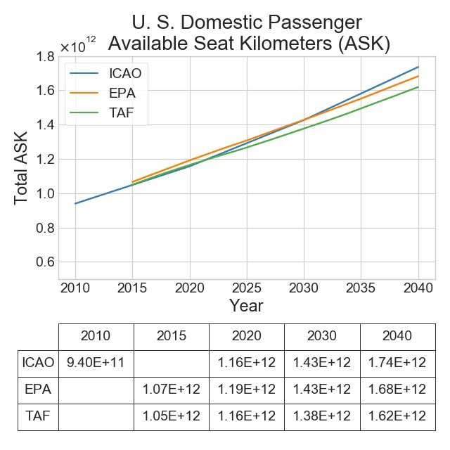
Table of Contents

Contents
1 Introduction ............................................................................................................................. 3
2 Methodology of the EPA Emissions Inventory and Stringency Analysis ............................... 5
 2.1 Fleet Evolution Model and Data Sources......................................................................... 6
 2.2 Full Flight Simulation with PIANO and Unit Flight Matrix.......................................... 12
 2.3 Inventory Modeling and Stringency Analysis................................................................ 14
3 Modeling Results for Fleet Evolution, Emission Inventories and Stringency Analyses ....... 15
 3.1 Fleet Evolution Results .................................................................................................. 16
 3.2 Baseline Emissions......................................................................................................... 23
 3.3 Stringency Analysis of U.S. and Global CO2 Emission Impacts ................................... 25
4 Sensitivity Case Studies......................................................................................................... 28
 4.1 Scenario 3 Sensitivity to Continuous Improvement....................................................... 28
 4.2 Scenario 3 Sensitivity to Extending Production of A380 and B767-3ERF to 2030 ...... 32
 4.3 Scenario 3 Sensitivity to Combined Effects of Continuous Improvement and Extended
 Production ................................................................................................................................. 34
 4.4 Similar Sensitivity Studies for Scenarios 1 and 2 ......................................................... 38
5 Conclusions ........................................................................................................................... 41
Appendix A Fleet Evolution Modeling Processes ................................................................... 42
1. Datasets.................................................................................................................................. 42
2. Database Filtering .................................................................................................................. 42
3. Growth Rate Calculation ....................................................................................................... 43
4. Retirement Rate Calculation.................................................................................................. 44
5. Growth and Replacement (G&R) Fleet ................................................................................. 45
6. Growth Operations – Market Demand Allocation ................................................................ 45
7. Fuel Burn Calculation............................................................................................................ 46
8. ICF Continuous Metric Value Forecast ................................................................................. 47
9. Stringency Analysis – Tech Response................................................................................... 47
Appendix B QUESTIONS FROM PEER REVIEWERS AND WRITTEN EPA RESPONSES
 49

 1

Appendix C Supplementary Materials..................................................................................... 52
1 ACCODE to PIANO Airplane Mapping ............................................................................... 52
2 Growth Forecast Numbers and Sources ................................................................................ 56
3 Growth and Replacement Operations by Fleet Family ......................................................... 57
4 Further Sensitivity Studies..................................................................................................... 58
 4.1 Great Circle Distance Scaling ........................................................................................ 58
 4.2 Payload Factor Sensitivity.............................................................................................. 58
 4.3 High/Low Growth Traffic Estimates.............................................................................. 59
 4.4 High/Low Technology Feasibility ................................................................................. 60

 2

1 Introduction
 Aviation is a major mode of transportation for connecting people and materials given its
advantage in speed and long-distance transport capability. Economically, it contributes to more
than 5% of U.S. GDP, 10 million U.S. jobs, $1.6 trillion of U.S. economic activities, and $60
billion of U.S. trade balance annually. However, airplanes are also a significant emission source
and air traffic is growing fast, globally, at a rate of 4-5% per year 1. Thus, it is important to
assess the airplane emissions inventory and potential environmental impacts.
 The first comprehensive global aviation emissions inventory was developed by National
Aeronautics and Space Administration (NASA) for 1992 2 and then 1999 3. Federal Aviation
Administration (FAA) in conjunction with Volpe Center of the Department of Transportation
subsequently developed a System for Assessing Aviation Global Emissions (SAGE) for 2000-
2004 4 inventories and later extended to 2005 5. Similar European efforts resulted in a global
aviation emissions inventories for 2002 and a forecast for 2025 6. These early works had led to
the development of the first International Civil Aviation Organization’s (ICAO) Environmental
Trends Report in 2010. ICAO has kept this Environmental Trends Report updated every three
years ever since, the latest one being the 2019 Environmental Report7. Beyond these official
global aviation emission inventories, increasingly there are inventories developed by academic
and independent initiatives based on diverse data sources and models with varying degree of
sophistication, coverage, and timeliness8 9 10 11.
 EPA had worked with the FAA and other stakeholders since 2010 to develop the first-ever
international CO2 standards for airplanes under the auspices of the ICAO’s Committee on
Aviation Environmental Protection (CAEP). This effort led to the agreement by CAEP on the
international CO2 standards in 2016, and ICAO formally adopted these standards in 2017. The
ICAO emissions standards are not self-implementing for individual nations, but these standards
must be implemented through domestic regulation.
 In 2016, the Environmental Protection Agency (EPA) issued endangerment and contribution
findings for aircraft engine greenhouse (GHG) emissions. These findings triggered EPA’s duty
under section 231 of the Clean Air Act to promulgate emission standards applicable to GHG
emissions from the classes of aircraft engines included in the findings. The EPA anticipates
moving forward on standards that would be at least as stringent as ICAO’s standards.
 To inform the U.S. domestic regulation, EPA conducts thorough technical analyses to
quantify the impact of the standard. Since much of ICAO regulatory impact analysis and data
are proprietary, EPA conducted an independent analysis with publicly available data so all
stakeholders would be able to understand how the agency derived its decisions. This report
documents the development of EPA’s emission inventory analysis including all data sources,
methodologies, and model assumptions.
 The EPA analysis focuses primarily on modeling the U.S. GHG emissions inventory. Since
aviation is an international industry and all major airplane and airplane engine manufacturers sell
their products globally, we also analyze the global fleet evolution and emissions inventories for
reference -- albeit traffic growth and fleet evolution outside of the U.S are modeled at a much
less detailed level.

 3

In developing the inputs to our model, the agency contracted with ICF to conduct an
independent airplane/engine technology analysis of fuel burn improvement for the period of
2010-2040. The agency uses this technology forecast as the basis for our impact assessment.
We also conducted sensitivity analyses to evaluate the effects of various model assumptions on
our results.
 The previous draft of this report (March 2019 version) was peer-reviewed through external
letter reviews by multiple independent subject matter experts, including experts from academia
and other government agencies, as well as independent technical experts12. The report was
updated based on the feedback received from the peer reviewers.

 4

2 Methodology of the EPA Emissions Inventory and Stringency
 Analysis
 The methodologies the agency uses to assess the impacts of the proposed standards and
alternative stringency scenarios are summarized in the flow chart shown in Figure 1. Essentially,
the approach is to compare the emissions inventory of a baseline (business-as-usual case in the
absence of standards) with those under various stringency scenarios.

 Figure 1 The flow chart diagram for EPA's emissions inventory and stringency analysis

 The first step of the EPA emissions inventory and stringency analysis is to develop an
inventory baseline by evolving the base year operations to future year operations emulating the
market driven fleet renewal process without any stringency requirements. This no stringency
baseline of operations and emissions is developed for the analysis period of 2015 to 2040. Our
approach to developing the baseline is to estimate the growth and retirement rates of future year
operations based on flights with unique route (origin-destination or OD-pair) and airplane
combinations in the base year operations. The growth and retirement rates for each of the unique
base year operations determine the future year market demand, which is then allocated to
available airplanes in a Growth and Replacement (G&R) database13.
 The growth and retirement rates over the analysis period are obviously a function of
macroeconomic factors like fuel price, materials prices and economic growth. These economic
factors are not considered explicitly in our analysis, but they are embedded in the traffic growth
forecast and retirement rates data (described in Appendix A) as inputs to the EPA analysis.
Together with the residual operations from the base year legacy airplanes, these G&R operations
constitute all the operations by the renewed in-service fleet for every future year.

 5

The same method is applied to define fleet evolutions under various stringency scenarios.
The only difference is under stringencies, we need to take technology responses into
consideration. The airplanes affected by a stringency requirement could either be modified to
meet the standard or removed from production without a response.
 Once the flight activities for all analysis scenarios are defined by the fleet evolution module,
we then compute fuel burn and CO2 emissions inventories for all the scenarios by simulating
these flights with a physics-based airplane performance model known as PIANO 14. The
differences between the baseline and various stringency scenarios are used for assessing the
impacts of the stringencies.
 The computational processes are grouped into three distinct modules as shown in Figure 1.
More detailed accounts of the methods, assumptions and data sources used for these three
computational modules are given below.

 2.1 Fleet Evolution Model and Data Sources
 The EPA fleet evolution model focuses on U.S. aviation, including both domestic and
international flights. U.S. international flights are defined as flights originating from the U.S.,
but landing outside the U.S. Flights originating outside the U.S. are not included in the U.S.
inventory. The EPA fleet evolution model is based on FAA 2015 Inventory Database 15 for base
year flight activities and FAA’s 2015-2040 Terminal Area Forecast16 (TAF) for future year
traffic growth.
 The FAA 2015 Inventory Database is a comprehensive global flight dataset. Its U.S. based
flights have been used as part of the high-fidelity sources for EPA's official annual GHG and
Sinks report since 199017. Globally, the 2015 inventory database contains 39,708,418 flights in
which 13,508,800 are originated from the U.S. Among the U.S. flights, 1,288,657 are by piston
engine aircraft, 341,078 are military operations and 1,393,125 are by small aircraft with
maximum zero fuel weight less than 6000 lbs. In our analysis, we exclude military, piston
engine aircraft and small light weight aircraft. Excluding these three aircraft categories that are
not subject to the standard, the database still contains 11,624,811 flights, 1,027,296,998 total
seats, 1,995,887,786,045 available seat kilometer (ASK) and 36,424,613,164 available tonne
kilometer (ATK) in the modeled 2015 U.S. operations.
 Likewise, TAF is a comprehensive traffic growth forecast dataset for commercial operations
in both U.S. domestic and international markets. The 2015-2040 TAF used in this analysis
contains growth forecast for both passenger and freighter markets based on origin-destination
airport pair and airplane type. In order to determine the growth rate of a base year operation, the
base year operation has to be mappedi from the 2015 Inventory Database to a corresponding
TAF market defined by market type (passenger or freighter), origin-destination airport pair, and

i
 In the absence of a set of keys (primary keys in 2015 Inventory and foreign keys from TAF) that can uniquely
identify the relationship between the two databases, a lookup table can be used to “map” the related information
from one database to another. The term “mapping” is used here in such context to apply appropriate growth rate
category (passenger or freighter) from TAF to the base year operations in 2015 Inventory via a lookup table such as
the one proposed in Table 1.

 6

airplane type. There is no unique mapping between these two databases. After some iterations
by trial and error and consultation with FAA, we have determined that a two-parameter mapping
using USAGE-CODE and SERVICE_TYPE works the best.
 The two-parameter mapping from the FAA 2015 Inventory Database to TAF is shown in
Table 1. USAGE_CODE and SERVICE_TYPE are the parameters in the 2015 Inventory
Database designed to identify the airplane usage category and the service type of any given flight
operation. They are used to identify the growth rate type (i.e., general aviation, passenger and
freighter under the GR_Map column of Table 1). The growth rate type in turn is used to
determine which data sources16,18,19,20 to look up for appropriate growth rate as will be elaborated
further below. Possible USAGE_CODEs are P for passenger, B for business, C for cargo, A for
attack/combat, and O for other. Possible SERVICE_TYPEs are C for commercial, G for general
aviation, F for freighter, M for military, O for other, and T for air taxi. For this analysis, we filter
out SERVICE_TYPEs of M (military), O (other), and T (air taxi) and only keep C (commercial),
G (general aviation), and F (freighter). Likewise, for USAGE_CODE, we filter out A
(attack/combat) and O (other) but keep P (passenger), B (business) and C (cargo) for this
analysis.
 Combinations of the remaining USAGE_CODE and SERVICE_TYPE subdivide the total
market into nine sub-market categories as shown in Table 1. The size of each sub-market
category based on the two-parameter mapping is summarized in Table 1 to give a sense of their
relative contributions to the overall fleet operations by available seat kilometer (TOTAL_ASK),
available tonne kilometer (TOTAL_ATK), and number of operations (TOTAL_OPS). In
consultation with FAA, these nine sub-markets are mapped into three growth rate types (under
the GR_Map column in Table 1) for the purpose of determining their growth rate forecast for
future year operations. Again, in GR_Map, G is for general aviation, F is for freighter and P is
for passenger. For U.S. passenger (P) and freighter (F) operations, TAF is used to determine the
growth rates for U.S. origin-destination (OD) pairs and airplane types from 2015 to 2040.
 Table 1 Two-parameter mapping from 2015 Inventory database to Growth Rate forecast databases

 USAGE_CODE SERVICE_TYPE GR_Map TOTAL_OPS TOTAL_ASK TOTAL_ATK
 B – Business C – Commercial G – General 5.8148E+05 4.5898E+09 9.8501E+08
 B F – Freight F – Freight 6.4350E+03 1.4580E+06 1.1399E+07
 B G – General G 1.3937E+06 1.3166E+10 2.8144E+09
 C – Cargo C F 2.2645E+05 2.8492E+10 3.7362E+10
 C F F 4.7665E+05 5.2309E+09 6.6587E+10
 C G G 9.6400E+03 6.1929E+08 1.8029E+09
 P – Passenger C P - Passenger 2.7432E+07 7.0697E+12 1.0836E+12
 P F F 3.1517E+05 8.8414E+10 2.6023E+10
 P G G 4.1658E+06 1.2560E+12 2.0427E+11

 In mapping the base year operations to TAF to determine their corresponding growth rate, if
there are exact OD-pair and airplane matches between the two databases, the exact TAF year-on-
year growth rates are applied to grow 2015 base year operations to future years. For cases
without exact matches, the growth rates of progressively higher-level aggregates will be used to

 7

grow the future year operations. For example, if there is no match in exact origin-destination
airport pair, the airport pair will be mapped to a route group (either domestic or international),
and the growth rate of the route group will be used instead to grow the operation. If there is no
match in airplane type (e.g., B737-8 MAX, B777-9X, etc.), the airplane category (e.g., narrow
body passenger, wide body freighter, etc.) as defined in the TAF will be used to map the growth
rate.
 Since general aviation is not covered in TAF, we use the forecasted growth rate of 1.6% for
U.S. turboprop operations based on FAA Aerospace Forecast (Fiscal Year 2017-2037) 18. For
U.S. business jet operations, we use the 3% CAGR (Compound Annual Growth Rate) forecasted
by the FAA Aerospace Forecast (Fiscal Year 2017-2037)18.
 For non-U.S. flights, we use an average compound annual growth rate of 4.5% for all
passenger operations and 4.2% for all freighters based on ICAO long term traffic forecast for
passenger and freighters 19. For non-U.S. business jet operations, we use the global average
growth rate of 5.4% based on Bombardier's Business Aircraft Market Forecast 2016-2025 20. A
summary of all the growth forecast sources and the growth rates used in this report is provided in
Appendix C-2 for various market segments.
 Given the classification of the two-parameter mapping table, we have determined that the
eighth row of the mapping table (where the USAGE_CODE = “P” and SERVICE_TYPE = “F”)
is converted freighters which are freighters converted from used passenger airplanes after the end
of their passenger services. These converted freighters are not subjected to the GHG standards ii,
so they are excluded from all inventory data reported below.
 The retirement rate of a specific airplane is determined by the age of the airplane and the
retirement curve associated with the airplane category. The retirement curve is the cumulative
fraction of retirement expected as the airplane ages. It goes from 0 to 1 as the airplane age
increases. The retirement curves can be expressed as a Sigmoid or Logistic function in the
form of
 1
 ( ) = 1/(1 + − )
where R is the retirement curve function, a and b are coefficients that change with airplane type
and t is the age of the airplane.
 The reason to choose this type of retirement function is because it is a well-behaved function
that matches well with historical retirement data of known airplane fleet. Figure 2 illustrates the
characteristic “S” shape of a fitted survival function, S(t), where S(t) = 1 – R(t). Note that the
ratio of the two coefficients in Equation 1, i.e., a/b, represents the half-life of the airplane fleet
where 50% of the fleet survives and 50% retires. The slope of the retirement curve (or percent
retired per year) at half-life is b/4. So, the larger the coefficient b is, the higher the rate of
retirement will be at half-life. The retirement curve is also an antisymmetric function with

ii
 The standards apply to new type and in-production airplanes after the effective dates of the standards, and the
standards do not apply to in-use airplanes, which include converted freighters.

 8

respect to the vertical axis, t = a/b and has long tails at both ends of the age distribution (for very
young and very old airplanes in the fleet).

 1970 1971
Narrow Body Passenger Retirement Curve 1972
 1974
 1973
 1975
 1976 1977
 1978 1979
 100% 1980 1981
 1982 1983
 1984 1985
 80% 1986 1987
 1988 1989
%Survived

 60% 1990 1991
 1992 1993
 1994 1995
 40% 1996 1997
 1998 1999
 2000 2001
 20% 2002 2003
 2004 2005
 2006 2007
 0% 2008 2009
 2010 2011
 0 10 20 30 40 2012 2013
 Airplane Age 2014
 CAEP10_NB
 2015
 BFSC

 Figure 2 The Retirement Curve of Narrow–Body Passenger Airplane Based on Ascend21 fleet data

 Retirement curves of major airplane categories used in this EPA analysis are derived
statistically based on data from the FlightGlobal’s Fleets Analyzer database 21 (also known as
ASCEND Online Fleets Database -- hereinafter “ASCEND”). Table 2 lists the numerical values
of these coefficients in the retirement curves for major airplane categories. The retirement
curves so established are consistent with published literature from Boeing and Avolon in terms
of the economic useful life of airplane categories. However, it is recognized from other sectors
(e.g., light duty vehicles) that the retirement curves are not necessarily exogenously fixed but
rather a function of the relative price of new versus used vehicles, fuel prices, repair costs, etc.
Furthermore, when regulations are vintage differentiated (i.e., when new vehicles are subject to
stricter requirements than older vintages), it has been shown that the economically useful life of
the existing fleet can be extended. The higher cost, and sometimes diminished performance of
compliant new vehicles makes it economically worthwhile to extend the life of older vehicles
that would otherwise have been retired. These extraneous factors, however, are not considered
in this analysis.

 9

Table 2 Retirement Curve coefficients by airplane category

 Airplane Category Description a b
 BJ Business Jet 6.265852341 0.150800149
 LQ Large Quad 5.611526057 0.223511259
 LQF Large Quad Freighter 6.905900732 0.205267334
 RJ Regional Jet 4.752779141 0.178659236
 SA Single Aisle 5.393337195 0.222210782
 SAF Single Aisle Freighter 6.905900732 0.205267334
 TA Twin Aisle 5.611526057 0.223511259
 TAF Twin Aisle Freighter 6.905900732 0.205267334
 TP Turboprop 3.477281304 0.103331799

 For each operation in the base year database (2015 Inventory), if the airplane tail number is
known, the retirement rate is based on exact age of the airplane from the ASCEND global fleet
database. If the airplane’s tail number is not known, the aggregated retirement rate of the next
level matching fleet (e.g., airplane category or airplane 'type' as defined by ASCEND) will be
used to calculate the retirement rates for future years.
 Combining the growth and retirement rates together, we can determine the total future year
market demands for each base year flight. These market demands are then allocated by equal
product market share iii to available G&R airplanes competing in the same market segment as the
base year flight. The available G&R airplanes for various market segments are based on the
technology responses developed by ICF, as documented in an ICF report.22 ICF technology
responses also include detailed information about the entry-into service year and the end-of-
production year for each current and future in-production airplanes out to 2040. The G&R
airplanes in each market segment are listed in Table 3. A detailed mapping of aircraft model
identification codes and PIANO aircraft models is provided in Appendix C-1.

 Table 3 The G&R airplane available in each market segment

 Market Description G&R Airplane Type
 Segment
 CBJ Corporate Jet A318-112/CJ, A319-133/CJ, B737-700IGW (BBJ), B737-8 (BBJ)
 FR Freighter A330-2F, B747-8F, B767-3ERF, B777-2LRF, TU204-F, AN74-F/PAX, B777-
 9xF, A330-800-NEOF
 LBJ Large Business Jet G-5000, G-6000, GVI, GULF5, Global 7000, Global 8000
 MBJ Medium Business CL-605, CL-850, FAL900LX, FAL7X, ERJLEG, GULF4
 Jet
 RJ_1 Small Regional Jet CRJ700, ERJ135-LR, ERJ145, MRJ-70
 RJ_2 Medium Regional CRJ900, ERJ175, AN-148-100E, AN-158, EJ-175 E2
 Jet

iii
 The EPA uses equal product market share (for all airplanes present in the G&R database), but attention has been
paid to make sure that competing manufacturers have reasonable representative products in the G&R database.

 10

RJ_3 Large Regional Jet CRJ1000, ERJ190, ERJ195, RRJ-95, RRJ-95LR, TU334, MRJ-90, ERJ-190 E2,
 ERJ-195 E2
 SA_1 Small Single Aisle A318-122, A319-133, B737-700, B737-700W, A319-NEO, B737-7MAX,
 CS100, CS300, MS-21-200
 SA_2 Medium Single A320-233, B737-800, B737-800W, A320-NEO, B737-8MAX, MS-21-300,
 Aisle C919ER
 SA_3 Large Single Aisle A321-211, B737-900ER, B737-900ERW, TU204-300, TU204SM, TU214,
 A321-NEO, B737-9MAX
 SBJ_1 Small Business CNA515B, CNA515C, EMB505, PC-24
 Jet_1
 SBJ_2 Small Business Learjet 40XR, Learjet 45XR, Learjet 60XR, CNA560-XLS, Learjet 70, Learjet
 Jet_2 75
 SBJ_3 Small Business CNA680, GULF150, CNA680-S
 Jet_3
 SBJ_4 Small Business CL-300, CNA750, FAL2000LX, G280, CNA750-X
 Jet_4
 TA_1 Small Twin Aisle A330-203, A330-303, B767-3ER, B787-8, A330-800NEO, A330-900-NEO
 TA_2 Medium Twin A350-800, A350-900, B787-9, B787-10
 Aisle
 TA_3 Large Twin Aisle B777-200ER, A350-1000, B777-8x
 TA_4 Very Large Twin A380-842, B747-8, B777-200LR, B777-300ER, B777-9x
 Aisle
 TP_1 Small Turboprop ATR42-5, IL114-100, AN-32P, AN140
 TP_2 Medium ATR72-2
 Turboprop
 TP_3 Large Turboprop Q400

 We allocate the market demand based on ASK for passenger operations, ATK for freighter
operations, and number of operations for business jets. Of course, given the number of seats for
passenger airplanes, payload capacity for freighters and the great circle distance for each flight,
all these parameters can be converted to a common activity measure, i.e., number of operations.
The formula for calculating number of operations for any out years is given in Equation 2.
 2
 GR(y) + RET(y)
 NOP(y) = (2015)
 N(c, y)

 where NOP(y) is number of operations in year y,
 GR(y) is the year over year growth rate in year y expressed as a fraction of the
base year operations
 RET(y) is the year over year retirement rate in year y expressed as a fraction of
the base year operations

 N(c,y) is the number of available airplane in market segment c and year y

 11

ICF technology response includes continuous improvement in metric value 23,iv (MV) for all
G&R airplanes from 2010 v to 2040. ICF technology responses also include estimated metric
value improvements for long-term replacement airplanes beyond the end of production of current
in-production and project airplanes. This is meant to establish a baseline where current in-
production airplanes are improving continuously and new type airplanes are introduced
periodically to replace airplane models that are going out of production due to market
competition. In order to capture this dynamic changing of airplane efficiency improvements, our
fleet evolution model tracks the market share of every new-in-service airplanes entering the fleet
each year and applies the annual fuel efficiency improvement -- via an adjustment factor
according to the vintage year of the airplanes in the fleet. For stringency analysis, if an airplane
fails a stringency limit and needs to improve its MV to comply with the standard, we apply the
adjustment factor in the same manner to establish the emissions under the influence of the
stringency limit.

 2.2 Full Flight Simulation with PIANO and Unit Flight Matrix
 The purpose of the full flight simulation module is to calculate instantaneous and cumulative
fuel burn, flight distance, flight altitude, flight time, and emissions by modeling airplane
performance for standardized flight trajectories and operational modes. PIANO version 5.4 was
used for all flight simulations. PIANO is a physics-based airplane performance model used
widely by industry, research institutes, non-governmental organizations and government
agencies to assess airplane performance metrics such as fuel efficiency and emissions
characteristics based on airplane types and engine types. PIANO v5.4 (2017 build) has 591
airplane models (including many project airplanes still under development, e.g., B777-9X) and
56 engine types in its airplane and engine databases. We use these comprehensive airplane and
engine data to model airplane performance for all phases of flight from gate to gate including
taxi-out, take-off, climb, cruise, descent, approach, landing and taxi-in in this analysis.
 To simplify the computation, we made a few modeling assumptions. 1) Assume airplanes fly
the great circle distance vi (which is the shortest distance along surface of the earth between two

iv
 The metric value is a certified airplane fuel efficiency value defined by ICAO’s Annex 16, Volume III and the
Environmental Technical Manual, Volume III. An airplane’s metric value is defined as the average of 1/(SAR*
RGF0.24) evaluated at three test points, where SAR is the Specific Air Range measuring the distance an airplane
travels in the cruise phase per unit of fuel consumed and RGF is the Reference Geometry Factor based on a
measurement of airplane fuselage size derived from a two-dimensional projection of the fuselage. The three test
points are defined by three airplane gross masses, i.e., high, mid and low gross masses. The high gross mass is
defined as 0.92*MTOM, where MTOM is the highest maximum take-off mass of all variants in the airplane type
design. The low gross mass is defined as 0.45*MTOM + 0.63*MTOM0.924. The mid gross mass is the average of
the high and low gross masses.
v
 For this analysis, with 2015 as the base year, we only use the continuous improvement data from 2015 to 2040.
vi
 Correction for great circle distance (GCD) can be made by an adjustment factor of 4% to 10% at the fleet level or
by adding a discrete detour distance for certain length of flights as used in the ICAO carbon calculator to account for
the difference between actual flight distance and the great circle distance. Appendix C-4.1 includes a sensitivity
study where the emission results are scaled by a constant adjustment factor for a better estimate of the annualized
global fleet emissions with realistic flight paths. This adjustment, which raises all emissions by the same factor,
does not change any conclusions of our analyses given the constant adjustment factor. Given accurate flight path

 12

airports) for each origin-destination (OD) pair. 2) Assume still air flights and ignore weather or
jet stream effects. 3) Assume no delays in takeoff, landing, en-route and other related flight
operations. 4) Assume a load factor of 75% vii maximum payload capacity for all flights except
for business jet where 50% is assumed. 5) Use the PIANO default reserve fuel rule viii for a given
airplane type. 6) Assume a one-to-one relationship between metric value improvement and fuel
burn improvement for airplanes with better fuel efficiency technology insertions (or technology
responses). Note that additional clarifications to peer reviewers’ questions about our model
assumptions are provided in Appendix B.
 When jet fuel is consumed in an engine, the vast majority of the carbon in the fuel reacts with
oxygen to form CO2. To convert fuel consumption to CO2 emissions, we used the conversion
factor of 3.16 kg/kg fuel for CO2 emissions based on ICAO Doc 9889 24 for typical commercial
jet fuels. To convert to the six well-mixed GHG emissions, we used 3.19 kg/kg fuel for CO2
equivalent emissions. It is important to note that in regard to the six well-mixed GHGs (CO2,
methane, nitrous oxide, hydrofluorocarbons, perfluorocarbons, and sulfur hexafluoride), only
two of these gases -- CO2 and nitrous oxide (N2O) -- are reported (or emitted) for airplanes and
airplane engines. The method for calculating CO2 equivalent emissions is to first calculate N2O
emissions based on SAE AIR 5715, entitled “Procedures for the Calculation of Airplane
Emissions” 25, and then to find the conversion factor for N2O to CO2 based on the 100-year
global warming potential factor from the EPA publication “Emissions Factors for Greenhouse
Gas Inventories”26.
 Given the flight activities defined by the fleet evolution module above, we generate a unit
flight matrix to summarize all the PIANO outputs of fuel burn, flight distance, flight time,
emissions, etc. for all flights uniquely defined by a combination of departure and arrival airports,
airplane types, and engine types. This matrix includes millions of flights and forms the basis for
all of the stringency scenarios and sensitivity studies. To reduce the computational workload of
such a huge task in the stringency analysis, we pre-calculate these full flight simulation results
and store them in a database of 50 distances and 50 payloads for each airplane and engine

data, an accurate adjustment factor can always be established, but it is less important for the stringency analysis.
Thus, the GCD assumption is clearly justifiable for the purpose of this report.
vii
 Additional load factors of 85% and 95% has been included as sensitivity studies in Appendix C-4.2. It turns out
that an increase of the load factor from 75% to 95% would increase the GHG emission by about 4% at the global
fleet level. This result is because load factor is held constant for each of these sensitivity cases and the fleet
evolution from the same base year operations and the same growth rate forecast would yield the same fleet
operations in all future years independent of the load factor assumption. Since the base year operation is fixed (as
input to our model), different load factor assumptions imply different base year RPK/FTK which would then grow
to future years at prescribed growth rate independent of the load factor assumption. Hence, the net effect of the load
factor assumption under this modeling framework is to increase the aircraft payload and weight resulting in higher
emissions for all cases (baseline and stringencies). Similar to the GCD assumption described above, it does not
change any conclusions of our analyses except raising emissions for all flights.
viii
 For typical medium/long-haul airplanes, the default reserve settings are for a 200 nautical mile diversion, 30
minutes of hold, plus a 5% contingency on mission fuel. Depending on airplane types, other reserve rules such as
U.S. short-haul, European short-haul, and National Business Aviation Association-Instrument Flight Rules (NBAA-
IFR) or Douglas rules are used as well.

 13

combination. The millions of flights in the unit flight matrix are interpolated from the 50x50
flight distance/payload database.

 2.3 Inventory Modeling and Stringency Analysis
 The GHG emissions calculation involves summing the outputs from the first two modules for
every flight in the database. This is done globally, and the U.S. portion is segregated from the
global dataset. The same calculation is done for the baseline and all the stringency scenarios.
When a surrogate airplane is used to model any airplane that is not in the PIANO database or
when a technology response is required for any airplane to pass a stringency limit, an adjustment
factor is also applied to model the expected performance of the intended airplane and technology
responses.
 The differences between the emissions inventories of various stringency scenarios and that of
the baseline provide the quantitative measures for the agency to assess the impacts of the
stringency options.

 14

3 Modeling Results for Fleet Evolution, Emission Inventories and
 Stringency Analyses
 The EPA fleet evolution model aims to develop future operations of the overall airplane fleet
based on the base year operations assuming a fixed network structure (no new routes or time
varying network configurations). We use a very simple market allocation method in which each
competing airplane within a market segment is given an equal market share. The market
allocation is based on airplane types and their operations measured in available seat kilometer
(ASK) or available tonne kilometer (ATK) or number of operations since they directly determine
the emissions output. We are not tracking flights and airplane deliveries at individual airplane
operator or airline level.
 In developing future year operations, all growth and replacement (G&R) operations and
residual legacy operations in future years are expressed in fractions of the base year operations in
our analysis. The growth and replacement operations come from new airplanes entering into
service to fill the market demands from increased air traffic and retirement of in-service fleet in
future years. The residual legacy operations are the remaining base year operations expected in
future years after retirement of a portion of the base year fleet.
 The market allocation of all G&R operations is applied to each individual flight in the base
year. Together with the residual operations from the base year, the total fleet operations in any
given year are made up of three parts, i.e., growth, retirement and residual operations. This is
true at any aggregate levels from individual flight to total global fleet. To illustrate the
relationship between base year operations and growth retirement and residual operations in
future years, the overall global fleet growth and replacement operations are depicted as an
example in Figure 3ix, where the lower line defines the residual (or remaining) operations while
the upper line defines the growth projection. The area between the base year operations (the
dashed horizontal line) and the growth line is growth operations. The area between the base year
operations and the residual line is the retirement operations. The area below the residual line is
the residual operations from the legacy fleet of the base year. The combined growth and
retirement operations in each year will be the total annual market demands that need to be filled
by G&R airplanes. The G&R fleet in any future year is comprised of G&R airplanes entering in
service from all previous years. The new enter-into-service airplanes themselves will retire
according to their respective retirement curves. Thus, the market share and distribution of
operations among the in-service fleet change from year to year. Our fleet evolution model tracks
these changes for each G&R airplane type and each enter-into-service year. Thus, we are able to
assign proper year to year improvements according to the year a G&R airplane enters into
service. Fleet evolution results and baseline emissions all depend on the exact age distribution of
the G&R fleet.

ix
 Additional charts depicting growth and replacement operations by fleet family are provided in Appendix C-3 for
reference.

 15

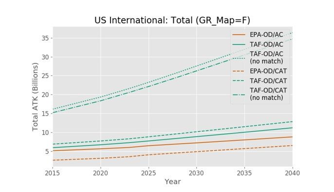
Figure 3 Global total growth and replacement operations in years 2015-2040

 3.1 Fleet Evolution Results
 Fleet evolution defines how the future fleet is composed and how future fleet operations are
distributed based on the operations of a base year and the market growth forecast from the base
year. It is the basis for calculating future year emissions and evaluating the impact of stringency
scenarios. The fleet evolution of the EPA analysis is developed independently of the ICAO
analysis. Per discussions in section 2, it is based on FAA's 2015 inventory database for the base
year operations and FAA's 2015-2040 TAF for future traffic growth. Since it is developed
independently, it is not directly comparable to the ICAO dataset. Nevertheless, we will compare
our fleet evolution results with ICAO and TAF data for a consistency check. There are no right
or wrong results in this comparison, but any outstanding differences may warrant some
discussion to ensure that they will not skew the results and affect the policy decisions in an
unexplainable manner.
 Figure 4 compares the EPA fleet evolution results with ICAO results. The EPA analysis
results are close to ICAO results, but differ by up to 10% in the analysis period of 2015-2040.
This is expected because there are many fundamental differences between the two analyses.
First, the EPA fleet evolution is based on FAA 2015 Inventory Database, while ICAO's fleet

 16

evolution is based on 2010 COD (Common Operations Database) 27. Second, the EPA growth
forecast is based on FAA 2015-2040 Terminal Area Forecast (TAF), while the ICAO growth
forecast is based on CAEP-FESGx consensus traffic forecast and industry provided fleet forecast
for passenger, freight and business jets for 2010-2040. Thus, the two fleet evolution models are
based on different data sources in both the base year operation and the growth rate forecast.
Coming within 10% differences in a 25-year span confirms that the two fleet evolution models
behave reasonably close to each other at the aggregate level despite the fact that the EPA fleet
evolution for the U.S. operations is very detailed based on the FAA data, while the ICAO model
treats all U.S. domestic operation as one uniform market.
 We also compare the EPA fleet evolution results with FAA TAF mainly to confirm that the
growth rates are consistent between the two approaches -- since EPA analysis growth rates are
sourced from TAF. Because the two databases (2015 Inventory and TAF) are developed and
maintained by different groups for different purposes using different data sources, some
differences exist in the base year operations, and these differences are most notable, in the
international freight operations. Many operations exist in one database, but not in the other and
vice versa.
 Our fleet evolution strategy is to evolve future year fleet operations solely based on FAA
2015 Inventory for the base year operations. Thus, in cases where the base year operations in
TAF are different from those in the 2015 Inventory, the TAF operational data are ignored. TAF
is only used to determine the growth rate of the fleet. The challenge for this strategy is in
mapping the base year operations correctly onto TAF to find the proper growth rates forecast for
the corresponding operations in future years. With this strategy, we will always get a unique
solution for future year operations with a given mapping of base year operations from 2015
Inventory to TAF, but there is no guarantee that the total operations so derived in any year will
be the same as the TAF. By using a two-parameter mapping, we were able to refine the grouping
of base year operations and improve the mapping between the two databases.
 Although some differences still exist between the two databases, further reconciliation is
beyond the scope of this project. By using the two-parameter mapping, we can also isolate the
converted freighter operations and exclude them from the stringency analysis because they
would not be subject to the proposed GHG standards. This exclusion also makes the freighter
results from the EPA analysis more comparable to ICAO's results, but other differences remain
as explained later.

x
 CAEP-FESG refers to the Forecasting and Economic Analysis Support Group which is the technical group tasked
to develop fleet growth forecast and cost effectiveness analyses for ICAO standards.

 17

Figure 4 Comparison of U.S. Passenger fleet ASK of ICAO, EPA and TAF

 The U.S. passenger fleet operations of the three datasets match reasonably well as shown in
Figure 4. We observe higher growth rate for ICAO results in both U.S. domestic and
international operations compared to the results from the EPA analysis. The EPA analysis
growth rate is in between the other two results.

 Figure 5 Comparison of U.S. Turboprop fleet ASK of ICAO, EPA and TAF (note different scale on y-axis)

 18

The U.S. turboprop fleet operations of the three datasets match less well as shown in Figure 5.
The EPA analysis and TAF are reasonably close, while ICAO is about 50 to 100 percent higher
in ASK. The difference is not a major concern for fleet wide emissions because turboprop
emissions are less than 1% of the overall fleet emissions. The difference to ICAO data is even
less of a concern to U.S. emissions since the ICAO dataset is less detailed and less refined for the
U.S. domestic and international operations compared to the FAA-TAF dataset. Since the EPA
fleet evolution results matches well with the TAF data, it suggests our fleet evolution results for
turboprop are reasonable. Therefore, the emissions and stringency analysis will proceed with the
EPA fleet evolution results on this basis and ignore the discrepancy with the ICAO data for now.

 Figure 6 Comparison of U.S. Regional Jet fleet ASK of ICAO, EPA and TAF (note different scale on y-axis)

 Similar to turboprop, the U.S. regional jet operations of the three datasets match well between
EPA and TAF, but ICAO has about 10% to 30% higher ASK and higher growth rate as shown in
Figure 6. This difference again is less of a concern for fleet-wide emissions because the regional
jet emissions are a small fraction of the overall passenger fleet emissions. The difference to
ICAO data is even less of a concern to U.S. emissions since the ICAO regional jet dataset is less
detailed and less refined than TAF for the U.S. domestic and international operations. Given that
the EPA fleet evolution results match well with the high-fidelity FAA-TAF dataset, the fleet
evolution results for regional jets are fit for purpose of this analysis.

 19

Figure 7 Comparison of U.S. Freighter fleet number of operations for ICAO, EPA and TAF (note different
 scale on y-axis)

 Figure 7 shows that the three datasets for freighters are quite different in terms of number of
operations. To compare fleet evolution results for freighter operations from the three datasets,
there are, however, several factors to be considered. These factors are as follows: (1) ICAO
freighter operations are exclusively from widebody purpose-built freighters while EPA and TAF
include smaller freighter types and, (2) between EPA and TAF, TAF has even more small
airplane operations in its dataset than the EPA analysis, which is based on the FAA 2015
Inventory. Thus, the higher number of operations in Figure 7 does not necessarily translate into
higher freighter capacity in terms of ATK as shown in Figure 8. The ICAO activity dataset we
use does not contain payload capacity information, so we can only compare EPA with TAF for
ATK.
 It is clear from Figure 8 that the EPA analysis results match TAF results closely for U.S.
domestic freighter operations. This close agreement, however, is not observed in the U.S.
international freighter operations. In that case, the ATK of TAF is more than twice the ATK of
the EPA analysis because possibly many U.S international freighter operations present in TAF
are missing in the 2015 Inventory from which the EPA ATK is derived. Figure 9 illustrates
some evidence supporting this hypothesis by separating out the operations in TAF with and
without origin-destination (OD) pair, airplane (AC), and airplane category (CAT) matches to the
EPA analysis (or FAA 2015 Inventory on which the EPA analysis is based). It is clear from
Figure 9 that a large part (the top two lines) of TAF U.S. international freight operations has no
matching OD/AC or OD/CAT in the EPA analysis. Given our methodology is to use the FAA
2015 Inventory as the basis to grow future year activities with TAF growth forecast, this
difference, although notable and maybe worthy of further investigations, does not affect our
ability to evolve all future freight operations based solely on freighter flights in the FAA 2015
Inventory. Further reconciliation between TAF and 2015 Inventory is beyond the scope of this
 20

project. For the purpose of this analysis, the EPA fleet evolution results will be used exclusively
for all the further stringency and impact analysis.

 Figure 8 Comparison of U.S. Freighter fleet ATK of EPA and TAF

 Figure 9 Total ATK of subsets of flights in EPA and TAF with and without match origin-destination pair
 (OD), airplane type (AC) and airplane category (CAT)

 21

Figure 10 Comparison of U.S. Business Jet fleet number of operations for ICAO and EPA (note different
 scale on y-axis)

 The business jet operations of ICAO and EPA analyses have similar 2010/2015 base year
operations, but different growth rates as shown in Figure 10. Comparing to EPA, ICAO appears
to underestimate the growth rate of U.S. domestic business jet operations and overestimate the
growth rate of U.S. international business jet operations. A higher growth rate of fleet operations
increases the G&R fleet faster over time, so it tends to amplify the impact of the standards.
Conversely, a lower growth rate of fleet operations depresses G&R fleet growth and tends to
lower the impact of the standards. Nevertheless, the effect of this baseline uncertainty is only
secondary since the stringency impact, as measured by the difference to the baseline, will be less
sensitive to the baseline uncertainty. More importantly, the rank order of stringency scenarios in
terms of emission reductions is typically not affected by the uncertainty in the baseline.
Although the agency recognizes the problem with the general lack of detailed and reliable
growth forecast data sources for subcategories like turboprop and business jet, we do not believe
that the uncertainty in these data will alter any conclusion of the analysis.

 3.1.1 Conclusions of the Fleet Evolution Results
 Overall, the EPA fleet evolution results agree quite well with ICAO and TAF for all
passenger operations in terms of ASK. For turboprop and regional jet operations, ICAO appears
to overestimate the U.S. domestic and U.S. international operations, but the EPA analysis agrees
well with TAF in all these operations. For freighter operations, the EPA analysis and TAF have
many small airplanes included, while ICAO is limited to widebody purpose- built freighters
only. The EPA analysis agrees well with TAF in U.S. domestic freighter operations in terms of
ATK, but it contains significantly fewer operations than TAF in U.S. international freighter
operations due to differences in the base year datasets. For business jet operations, the EPA
analysis and ICAO have similar base year operations, but different growth rates which cause
significant differences in out years. In absence of more reliable data sources for business jet
growth forecast, EPA will proceed with the current forecast sources from FAA and Bombardier
 22

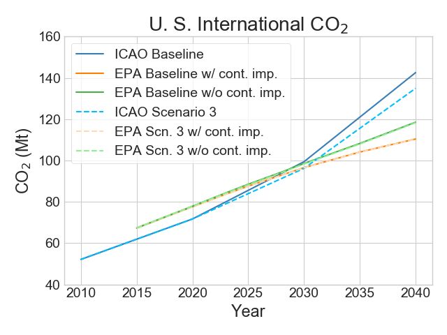
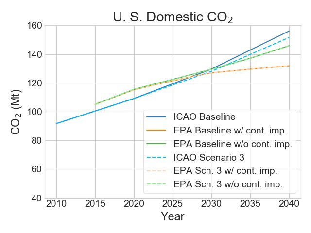
for the EPA analysis. The uncertainty in the baseline forecast is noted, but considered to be
secondary for the stringency assessment.

 3.2 Baseline Emissions
 The baseline CO2 emissions inventories are estimated in this EPA analysis for 2015, 2020,
2023, 2025, 2028, 2030, 2035 and 2040 using PIANO (the airplane performance model), and the
emissions inventory method is described in Section 2 along with each year’s activities data
derived from the fleet evolution model. The baseline CO2 emissions for global, U.S. total, U.S.
domestic, and U.S. international flights are shown in Figure 11 based on outputs from the fleet
evolution model.
 In each of the plots contained in Figure 11, there are three baselines plotted. These include
the primary analysis (labeled as "CO2") and two sensitivity scenarios (labeled as "CO2 without
continuous improvement" and "frozen fleet assumption"). The top line is the frozen fleet
baseline, which is basically an emission baseline growing at the rate of traffic growth assuming
constant fuel efficiency in the fleet (i.e., no fleet evolution). The second line is the no continuous
improvement baseline where the fuel efficiency of the fleet is benefitted from the infusion of
newer airplanes from fleet evolution, but the new airplanes entering into the fleet are assumed to
be static and not improving over the analysis period (2015-2040). The third line is the business-
as-usual (BAU) baseline, where the fleet fuel efficiency would benefit from both fleet evolution
with the new airplanes entering the fleet and business-as-usual improvement of the new in-
production airplanes.
 These emissions inventory baselines thus provide a quantitative measure for the effects of
model assumptions on fleet evolution and continuous improvement. The business-as-usual
baseline incorporates all market driven emissions reductions factors. It is used as the primary
baseline for this EPA analysis. The other two baselines are useful references for illustrating the
effects of fleet evolution and continuous improvement.
 Comparing the baselines, the difference between the two higher baselines in Figure 11 is due
to fleet evolution. Even for G&R airplanes without continuous improvement, the powerful effect
of fleet renewal is clearly evident in emissions inventories of all markets (global, U.S. Domestic
and U.S. international)xi. The difference between the lower two baselines Figure 11 is the effect
of continuous improvement since they have identical fleet evolution.
 These baselines are established with no stringency inputs, nevertheless they provide very
powerful insights into the drivers for emissions inventories and trends. The difference in global
CO2 emission between the BAU and the frozen fleet baselines in 2040 alone is about 400 Mt, a
significant emissions reduction achievable by market force alone.
 It is worth noting that the US domestic market is relatively mature with lower growth rate
than most international markets. This slower growth rate has obvious consequences in the

xi
 It may be worth mentioning that the ICAO baseline is in between these two higher baselines since the ICAO
baseline includes limited fleet evolution with a short list of transition pairs for which replacement airplanes had been
identified at the time of the ICAO CO2 analysis23.

 23

growth rate of the US domestic CO2 emissions baseline, which is projected with a very slow
growth rate by 2040 given the continuous improvement assumptions.

 Figure 11 Range of CO2 emissions baselines with various fleet evolution and continuous improvement
 assumptions

 3.2.1 Discussions for baseline modeling
 By modeling fleet evolution variables such as the end-of-production timing and continuous
improvements explicitly, the agency believes that the business-as-usual baseline would provide

 24

more accurate assessment of the impacts of the standards on emissions. This comprehensive
model can be a powerful tool to understand the effect of these model variables.
 One might argue how fast new technology could infuse into the fleet and how much market-
driven business-as-usual improvement can be assumed are all inherently uncertain. However,
given accurate inputs for fleet evolution and continuous improvement, the baseline inventory can
be better assessed for the real-world performance of all fleets (global, domestic or international).
 To help develop this baseline, the EPA contracted ICF to conduct an independent analysis to
develop a credible fleet evolution and technology response forecast. This forecast considered
both near-term and long-term technological feasibility and market viability of available
technologies and costs for all the modeled G&R airplanes at individual airplane type and family
levels.
 Given these fleet evolution and efficiency improvement estimates, the agency believes that
the emissions inventory baseline established provides the best possible representation for the
performance of the global and U.S. fleet for assessing the impact of the proposed GHG
standards.
 It is traditionally assumed that the baseline does not matter for stringency analysis, because
the impact of the stringency is measured from stringency to baseline, the effects of baseline
choices tend to cancel out when the primary objective is just to compare the delta of stringency
and baseline. It can be shown that this assumption may not be true when some of the fleet
evolution assumptions affect the emission outputs of the baseline and stringency lines
differently. As a result, the output of the stringency analysis might be skewed and subsequently
influence the policy-making decisions.
 In conclusion, using the best possible estimate of a baseline would lead to a more accurate
assessment of the impact of the standards. The effects of fleet evolution, continuous
improvements, and technology responses on emissions inventory and emissions reductions are
discussed further in the following sections.

 3.3 Stringency Analysis of U.S. and Global CO2 Emission Impacts
The EPA main analysis includes three stringency scenarios, the proposed standard and two
alternatives. The primary scenario is the proposed standard, which is equivalent to the ICAO
CO2 standard. The two alternative scenarios are a pull-ahead (an earlier implementation of the
standard by the timing shown in Table 4) scenario at the same stringency (Scenario 2) and a
pull-ahead scenario at a higher stringency (Scenario 3). Table 4 lists the stringency levels and
implementation timing of the three stringency scenarios. See ICF Report22 for more detailed
description of these stringency scenarios. Detailed description on the definition of airplane fuel
efficiency metric valueiv and the measurement techniques and test procedures to determine pass
or fail status of an airplane against the GHG standards can be found in section V of the 2020
EPA Notice of Proposed Rulemaking for Control of Air Pollution from Airplanes and Airplane
Engines: GHG Emission Standards and Test Procedures.

 25