High-resolution quantification of atmospheric CO2 mixing ratios in the Greater Toronto Area, Canada - Atmos. Chem. Phys
←
→
Page content transcription
If your browser does not render page correctly, please read the page content below
Atmos. Chem. Phys., 18, 3387–3401, 2018
https://doi.org/10.5194/acp-18-3387-2018
© Author(s) 2018. This work is distributed under
the Creative Commons Attribution 4.0 License.

High-resolution quantification of atmospheric CO2 mixing
ratios in the Greater Toronto Area, Canada
Stephanie C. Pugliese1 , Jennifer G. Murphy1 , Felix R. Vogel2,4 , Michael D. Moran3 , Junhua Zhang3 , Qiong Zheng3 ,
Craig A. Stroud3 , Shuzhan Ren3 , Douglas Worthy4 , and Gregoire Broquet2
1 University
           of Toronto, Department of Chemistry, 80 St. George St, Toronto, ON, M5S 3H6, Canada
2 Laboratoire
            des Sciences du Climat et de L’Environnement, CEA-CNRS-UVSQ, Université de Paris-Saclay, France
3 Environment and Climate Change Canada, Air Quality Research Division, 4905 Dufferin St. Toronto,

ON, M3H 5T4, Canada
4 Environment and Climate Change Canada, Climate Research Division, 4905 Dufferin St. Toronto, ON, M3H 5T4, Canada

Correspondence: Jennifer G. Murphy (jmurphy@chem.utoronto.ca)

Received: 20 July 2017 – Discussion started: 26 July 2017
Revised: 31 December 2017 – Accepted: 18 January 2018 – Published: 8 March 2018

Abstract. Many stakeholders are seeking methods to reduce       ety of statistics such as correlation coefficient, root-mean-
carbon dioxide (CO2 ) emissions in urban areas, but reli-       square error, and mean bias. Furthermore, when run with the
able, high-resolution inventories are required to guide these   SOCE inventory, the model had improved ability to capture
efforts. We present the development of a high-resolution        the typical diurnal pattern of CO2 mixing ratios, particularly
CO2 inventory available for the Greater Toronto Area and        at the Downsview, Hanlan’s Point, and Egbert sites. In addi-
surrounding region in Southern Ontario, Canada (area of         tion to improved model–measurement agreement, the SOCE
∼ 2.8 × 10⁵ km2 , 26 % of the province of Ontario). The new     inventory offers a sectoral breakdown of emissions, allowing
SOCE (Southern Ontario CO2 Emissions) inventory is avail-       estimation of average time-of-day and day-of-week contri-
able at the 2.5 × 2.5 km spatial and hourly temporal resolu-    butions of different sectors. Our results show that at night,
tion and characterizes emissions from seven sectors: area,      emissions from residential and commercial natural-gas com-
residential natural-gas combustion, commercial natural-gas      bustion and other area sources can contribute > 80 % of the
combustion, point, marine, on-road, and off-road. To as-        CO2 enhancement, while during the day emissions from the
sess the accuracy of the SOCE inventory, we developed           on-road sector dominate, accounting for > 70 % of the en-
an observation–model framework using the GEM-MACH               hancement.
chemistry–transport model run on a high-resolution grid with
2.5 km grid spacing coupled to the Fossil Fuel Data Assim-
ilation System (FFDAS) v2 inventories for anthropogenic
CO2 emissions and the European Centre for Medium-Range          1   Introduction
Weather Forecasts (ECMWF) land carbon model C-TESSEL
for biogenic fluxes. A run using FFDAS for the Southern         Urban areas are sites of dense population and the intensity of
Ontario region was compared to a run in which its emis-         human activities (such as transportation, industry, and resi-
sions were replaced by the SOCE inventory. Simulated CO2        dential and commercial development) makes them hotspots
mixing ratios were compared against in situ measurements        for anthropogenic carbon dioxide (CO2 ) emissions. While
made at four sites in Southern Ontario – Downsview, Han-        occupying only 3 % of the total land area, urban areas are
lan’s Point, Egbert and Turkey Point – in 3 winter months,      locations of residence for 54 % of the global population and
January–March 2016. Model simulations had better agree-         are the source of 53–87 % of anthropogenic CO2 emissions
ment with measurements when using the SOCE inventory            globally (IPCC-WG3, 2014; WHO, 2015). When consider-
emissions versus other inventories, quantified using a vari-    ing Canada alone, the urban population accounts for an even
                                                                larger fraction of the total (81 % in 2011) (Statistics Canada,

Published by Copernicus Publications on behalf of the European Geosciences Union.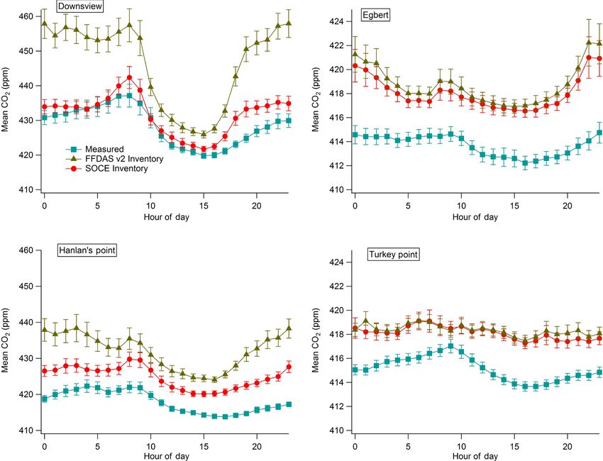
3388                                S. C. Pugliese et al.: High-resolution quantification of atmospheric CO2 mixing ratios

2011) while urban areas cover only 0.25 % of the land area        Successful examples of high-resolution CO2 inventory de-
(Statistics Canada, 2009). Recognizing their influence on the     velopment are available on the urban scale, such as the Air-
global carbon budget, many urban areas are seeking methods        parif inventory in Île-de-France (publicly available at http:
to reduce their anthropogenic CO2 emissions. The Greater          //www.airparif.asso.fr/en/index/index) and in Indianapolis,
Toronto Area (GTA) in southeastern Canada, for example,           Los Angeles, Salt Lake City, and Phoenix through the Hestia
has committed to the “Change is in the Air” initiative and is     project (Gurney et al., 2012); on the national scale, such as
a part of the C40 Cities Climate Leadership Group, both of        in China (Zhao et al., 2012); and on the global scale (Wang
which call to reduce CO2 emissions 30 % below 1990 lev-           et al., 2013). However, to our knowledge, there are currently
els by 2020 (C40 Cities, 2016; Framework for Public Re-           no studies that have quantified Canadian CO2 emissions at
view and Engagement, 2007). However, in order to effec-           the fine spatial and temporal resolution required for urban
tively guide anthropogenic CO2 mitigation strategies, reli-       analyses in Canada.
able inventories are needed, particularly at high spatial and        In an effort to address this gap, this study was focused on
temporal resolution, to gain a better understanding of the car-   quantifying CO2 emissions at a fine spatial and temporal res-
bon cycle (Gurney et al., 2009; Patarasuk et al., 2016). To our   olution in the GTA and Southern Ontario (we expanded the
knowledge, the only spatially disaggregated CO2 inventories       inventory beyond the urban area of the GTA so we could
available for use in the GTA are the EDGAR v.4.2 (Emission        exploit information on CO2 mixing ratios collected at rural
Database for Global Atmospheric Research) CO2 inventory           areas in Central and Southwestern Ontario, providing ad-
(available at annual, 0.1◦ × 0.1◦ resolution) (EDGAR, 2010)       ditional sites for inventory validation). We present the new
and the FFDAS v2 (Fossil Fuel Data Assimilation System)           high-resolution Southern Ontario CO2 Emissions (SOCE) in-
CO2 inventory (available at hourly, 0.1◦ × 0.1◦ resolution)       ventory, which quantifies CO2 emissions from seven source
(FFDAS, 2010), both which are limited in their spatial and/or     sectors (on-road, off-road, area, point, marine, residential,
temporal resolution and therefore are not well-suited for the     and commercial natural-gas combustion) at 2.5 km × 2.5 km
quantification and understanding of CO2 emissions at the ur-      spatial and hourly temporal resolution for an area covering
ban scale. The Canadian national CO2 inventory, in contrast,      ∼ 26 % of the province of Ontario (∼ 2.8 × 10⁵ km2 ). The
is only available at the provincial level (Environment Canada,    SOCE inventory was used in combination with the Envi-
2012).                                                            ronment and Climate Change Canada (ECCC) GEM-MACH
   Efforts to develop emission inventories at the fine spa-       chemistry–transport model to simulate CO2 mixing ratios
tial and temporal resolution required for urban-scale under-      in a domain including southeastern Canada and northeast-
standing of CO2 emissions have been driven by both policy-        ern USA (hereafter referred to as the “PanAm domain”) for
and science-related questions (Gurney et al., 2009; Patara-       comparison with in situ measurements made by the South-
suk et al., 2016). From a policy perspective, improving CO2       ern Ontario Greenhouse Gas Network. Until now, estimates
emission quantification is essential to independently evalu-      of anthropogenic CO2 emissions in the GTA were available
ate whether anthropogenic mitigation regulations are being        only from the EDGAR v.4.2 (EDGAR, 2010) and the FFDAS
effectively implemented. From a scientific perspective, gain-     v2 (FFDAS, 2010) inventories, which have very different an-
ing information about anthropogenic CO2 emissions from ur-        nual totals for this region (1.36 × 10⁸ vs. 1.05 × 10⁸ t CO2 ,
ban areas has been primarily motivated by atmospheric CO2         respectively). Therefore, we expect the results of this work
inversions, which are used to better understand the global        will improve our ability to quantify the emissions of CO2 in
carbon cycle (Gurney et al., 2009; Patarasuk et al., 2016).       the entire domain as well as the relative contributions of dif-
Regardless of the motivation, quantification of CO2 source–       ferent sectors, providing a more detailed characterization of
sink processes currently uses two techniques: the bottom-         the carbon budget in the GTA.
up approach and the top-down approach. In the bottom-
up approach, local-scale activity level information is com-
bined with appropriate emission factors to infer emission         2     Methods
rates. This method has been used widely to develop many
inventories (EDGAR, 2010; FFDAS, 2010; Gurney et al.,             2.1    Geographic domain
2009) but is limited by the accuracy of the input parameters.
Conversely, in the top-down approach, inverse modelling is        The geographic focus of this study was the GTA in South-
used to exploit the variability in atmospheric mixing ratios      ern Ontario, Canada. The GTA is the largest urban area
of CO2 to identify the source–sink distributions and magni-       in Canada; it comprises five municipalities, Toronto, Hal-
tudes; this method is limited by insufficient mixing ratio data   ton, Durham, Peel, and York, which together have a pop-
and uncertainties in simulating atmospheric transport (Pillai     ulation exceeding 6 million (Statistics Canada, 2012b). Al-
et al., 2011). Given current policy needs, a strategy using       though the GTA comprises only 0.07 % of Canadian land
solely bottom-up or top-down approaches is likely insuffi-        area, it represents over 17 % of the total population as a result
cient to evaluate CO2 emissions; rather, a synthesis of the       of rapid urbanization over the past few decades (Statistics
two methodologies is required (Miller and Michalak, 2016).        Canada, 2012b). Therefore, high-resolution characterization

Atmos. Chem. Phys., 18, 3387–3401, 2018                                            www.atmos-chem-phys.net/18/3387/2018/
S. C. Pugliese et al.: High-resolution quantification of atmospheric CO2 mixing ratios                                                   3389

                                                                              just south of the city of Toronto on the shore of Lake On-
                                                                              tario. Site details and instrument types used can be found
                                                                              in Table 1. CO2 measurements are collected as a part of
                                                                              ECCC’s Greenhouse Gas Observational Program. The mea-
                                                                              surement procedure follows a set of established principles
                                                                              and protocols outlined by a number of international agen-
                                                                              cies through recommendations of the Meeting on Carbon


                                                                              Dioxide, Other Greenhouse Gases, and Related Measure-
                                                                              ment Techniques, coordinated by the World Meteorological
                                                                              Organization (WMO) every 2 years.
                                                                                 The atmospheric CO2 observational program at the Eg-

       bert site is based on nondispersive infrared (NDIR) method-

              ology and fine-tuned for high-precision measurements (Wor-


                                                                              thy et al., 2005). A detailed description of the NDIR obser-


                                                                              vational system can be found in Worthy et al. (2005). The
                                                                              atmospheric CO2 observational programs at Turkey Point,
Figure 1. Total anthropogenic CO2 emissions for a weekday in                  Downsview, and Hanlan’s Point are based on cavity ring-
February 2010 estimated by the SOCE inventory for the province                down spectroscopy (CRDS). Each Picarro CRDS system is
of Ontario and by the FFDAS v2 inventory for the remainder of the             calibrated in the ECCC central calibration facility in Toronto
GEM-MACH PanAm domain. Locations of in situ measurements of                   before deployment to the field. The response function of
CO2 in the Southern Ontario Greenhouse Gas Network are shown in               the analyzer is determined against three calibrated standards
the inset (Downsview is a square, Egbert is a circle, Hanlan’s Point
                                                                              tanks (low, mid, high). The working (W) and target (T) tanks
is a triangle, Turkey Point is a diamond). The Downsview and Han-
lan’s Point sites are both located in the GTA. Unit: g CO2 s−1 grid
                                                                              assigned to the system are also included in the injection se-
cell−1 .                                                                      quence and calibrated. At each site, ambient measurements
                                                                              are made using two sample lines placed at the same level.
                                                                              Each sample line has separate dedicated sample pumps and
of CO2 emissions can help integrate climate policy with ur-                   driers (∼ −30 ◦ C). Pressurized aluminum 30 L gas cylin-
ban planning. This region is home to a network of measure-                    ders are used for the working and target tanks. The sample
ment sites providing long-term, publicly available datasets                   flow rate of the ambient and standard tank gases is set at
of atmospheric CO2 mixing ratio measurements (Sect. 2.2;                      ∼ 300 cc min−1 . The injection sequence consists of a target
Environment Canada, 2011) which can be used to evaluate                       and working tanks sequentially passed through the analyzer
model outputs and inventory estimates. In 2016 the govern-                    for 10 min each every 2 days. The ambient data from line 1
ment of Ontario released a Climate Change Action Plan,                        are passed through the analyzer for 18 h followed by line 2
which includes an endowment given to the Toronto Atmo-                        for 6 h. The line 1–line 2 sequence repeats one time before
spheric Fund of CAD 17 million to invest in strategies to re-                 the target and working tanks are again passed through the
duce greenhouse gas pollution in the GTA (Ontario, 2016).                     system. The working and target tanks are calibrated on site
Therefore this research can provide timely information on                     at least once per year against a single transfer standard trans-
the carbon budget in the GTA and help to implement effec-                     ported between the sites and the central laboratory facility
tive reduction strategies.                                                    in Toronto. The CO2 measurements from both the NDIR and
                                                                              CRDS analytical systems have a precision of around 0.1 ppm
2.2   The Southern Ontario Greenhouse Gas Network                             based on 1 min averages and are accurate to within 0.2 ppm.

Measurements of ambient CO2 dry air mixing ratios be-                         2.3   GEM-MACH chemistry–transport model
gan in 2005 in Southern Ontario at the Egbert station fol-
lowed by the Downsview station (2007), Turkey Point sta-                      In this project, we used the GEM-MACH (Global Environ-
tion (2012), and Hanlan’s Point station (2014) (Fig. 1). Mea-                 mental Multi-scale – Modelling Air quality and CHemistry)
surements were also temporarily made at a site in down-                       chemistry–transport model (CTM) (Gong et al., 2015; Moran
town Toronto, the Toronto Atmospheric Observatory (TAO)                       et al., 2013; Pavlovic et al., 2016; Talbot et al., 2008) to link
(43.7◦ N, 79.4◦ W), but the instrument was relocated from                     surface emission estimates and atmospheric mixing ratios.
this site in January 2016. Egbert is located ∼ 75 km north-                   GEM-MACH is an online CTM embedded within the Cana-
northwest of Toronto in a rural area, Downsview is located                    dian weather forecast model GEM (Côté et al., 1998a, b).
∼ 20 km north of downtown core of the city of Toronto in                      The configuration of GEM-MACH used in our study has 62
a populated suburban area, Turkey Point is located to the                     vertical levels from the surface to ∼ 1.45 hPa on a terrain-
southwest of the GTA in a rural area on the north shore of                    following staggered vertical grid for a log-hydrostatic pres-
Lake Erie, and Hanlan’s Point is located on Toronto Island,                   sure coordinate. The thickness of the lowest layer was 40 m.

www.atmos-chem-phys.net/18/3387/2018/                                                          Atmos. Chem. Phys., 18, 3387–3401, 2018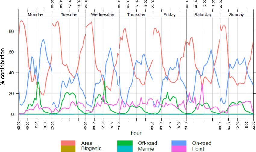
3390                                        S. C. Pugliese et al.: High-resolution quantification of atmospheric CO2 mixing ratios

Table 1. Summary of atmospheric measurement programs in Southern Canada operated by Environment and Climate Change Canada.

                                                                                                    Elevation             Intake     In situ
            Start date              Site name                        Coordinates                       (a.s.l.)           height     instrumentation
            March 2005              Egbert                44.231037◦ N, 79.783834◦ W                    251 m       3 m, 25 m∗        NDIR
            November 2010           Downsview             43.780491◦ N, 79.468010◦ W                    198 m             20 m        NDIR
            November 2012           Turkey Point          42.635368◦ N, 80.557659◦ W                    231 m             35 m        CRDS
            June 2014               Hanlan’s Point        43.612201◦ N, 79.388705◦ W                     87 m             10 m        CRDS
          ∗ At Egbert, a 25 m tower was installed in 9 March 2009. NDIR is nondispersive infrared. CRDS is cavity ring-down spectroscopy.

The PanAm domain used in our simulations, which includes                              GEM-MACH for this project to account for CO2 concentra-
Central and Southern Ontario as well as western Québec and                            tion fields associated with difference source sectors and the
the northeastern USA, is shown in Fig. 1. The PanAm do-                               lateral boundaries. The CO2 boundary conditions set at the
main has 524 × 424 grid cells in the horizontal on a rotated                          lateral and top edges of the domain were obtained from the
latitude–longitude grid with 2.5 km grid spacing and covers                           Monitoring Atmospheric Composition and Climate (MACC)
an area of approximately 1310 km × 1060 km (total domain                              global inversion, v.10.2 (http://www.gmes-atmosphere.eu/).
area is 1.39 × 10⁶ km2 ). A 24 h forecasting period was used                          Model-simulated specific humidity (q, kg kg−1 ) was used to
with a 60 s time step for each integration cycle. Meteoro-                            convert estimated CO2 mixing ratios to dry air mixing ratios.
logical fields (wind, temperature, humidity, etc.) were reini-                        CO2 dry air mixing ratios are hereafter referred to CO2 mix-
tialized every 24 h (i.e., after each model integration cycle);                       ing ratios.
chemical fields were carried forward from the previous inte-
gration cycle (i.e., perpetual forecast). Hourly meteorologi-
cal and chemical boundary conditions were provided by the                             2.4     High-resolution SOCE inventory development
ECCC operational 10 km GEM-MACH air quality forecast
model (Moran et al., 2015).
                                                                                      The high-resolution SOCE inventory was constructed pri-
   In our study, we simulated two scenarios of CO2 surface
                                                                                      marily from a pre-existing carbon monoxide (CO) inventory
fluxes:
                                                                                      developed by the Pollutant Inventories and Reporting Divi-
   Scenario 1 is characterized by the sum of the following:
                                                                                      sion (PIRD) of ECCC as part of the 2010 Canadian Air Pollu-
  – anthropogenic fossil fuel CO2 emissions within the                                tant Emissions Inventory (APEI). The CO inventory is a com-
    province of Ontario estimated by the SOCE inventory,                              prehensive national anthropogenic inventory that includes
    available at 2.5 km × 2.5 km spatial and hourly temporal                          emissions from area sources, point sources, on-road mobile
    resolution, as described in Sect. 2.4;                                            sources, and off-road mobile sources, including aircraft, lo-
                                                                                      comotive, and marine emissions for base year 2010 (Moran
  – anthropogenic fossil fuel CO2 emissions estimated by                              et al., 2015). This annual inventory at the provincial level
    the FFDAS v2 inventory (FFDAS, 2010) outside of the                               compiled by PIRD was transformed into model-ready emis-
    province of Ontario (province of Québec and USA),                                 sions files using the Sparse Matrix Operator Kernel Emis-
    available at 0.1◦ × 0.1◦ spatial and hourly temporal res-                         sions (SMOKE, https://www.cmascenter.org/smoke/) emis-
    olution;                                                                          sions processing system for spatial allocation (distribution
                                                                                      of non-point-source emissions to 2.5 km × 2.5 km (roughly
  – biogenic CO2 fluxes from the C-TESSEL land surface                                0.02◦ × 0.02◦ resolution) using spatial surrogate fields) and
    model, as described in Sect. 2.5.                                                 temporal allocation (conversion of inventory annual emis-
                                                                                      sion rates into hourly values) (Moran et al., 2015). Be-
  Scenario 2 is characterized by the sum of the following:                            cause Ontario CO emissions in the 2010 APEI were pro-
  – anthropogenic fossil fuel CO2 emissions estimated by                              cessed in separate steps with SMOKE by primary source sec-
    the FFDAS v2 inventory (FFDAS, 2010) for the entire                               tor, files of gridded hourly CO emissions fields were avail-
    domain, available at 0.1◦ × 0.1◦ spatial and hourly tem-                          able for seven different inventory sectors: area sources, point
    poral resolution;                                                                 sources, on-road mobile sources, off-road mobile sources,
                                                                                      marine sources, residential natural-gas sources, and com-
  – biogenic CO2 fluxes from the C-TESSEL land surface                                mercial natural-gas sources. The spatial and temporal allo-
    model, as described in Sect. 2.5.                                                 cations applied to these seven sectors were different, so in
                                                                                      effect they constitute a set of spatiotemporal emissions basis
CO2 is not a usual chemical species considered by GEM-                                functions. More detailed information about the CO inventory
MACH but a set of special inert tracer fields was added to                            compilation and subsequent processing has been provided

Atmos. Chem. Phys., 18, 3387–3401, 2018                                                                      www.atmos-chem-phys.net/18/3387/2018/
S. C. Pugliese et al.: High-resolution quantification of atmospheric CO2 mixing ratios 3391
elsewhere (Environment Canada, 2013; Moran et al., 2015; 2.4.2 Point emissions
PIRD, 2016).
The objective of our work was to calculate CO2 emissions Point emissions are stationary sources in which emissions
based on this processed, sector-specific, model-ready CO exit through a stack or identified exhaust. In the APEI CO
inventory for Ontario grid cells using sector-specific emis- inventory, the major emission sources in the point sector in-
sion ratios estimated by the Canadian National Inventory clude public electricity and heat production (1A1a), station-
Report (NIR) (Environment Canada, 2012). The NIR esti- ary combustion in manufacturing industries and construc-
mates CO2 and CO emissions using primarily bottom-up es- tion (1A2f), chemical industry (2B5a), pulp and paper (2D1),
timates; for example, emissions from industrial process are iron and steel production (2C1), and other metal production
estimated using production data reported directly by facili- (2C5). Unlike the area sector, we found that applying a sin-
ties whereas emissions from road transport activities are es- gle CO2 : CO ratio to every facility did not produce realis-
timated using vehicle population data, fuel consumption ra- tic CO2 emissions due to the negligible emissions of CO and
tios, and vehicle kilometres travelled as reported by Environ- therefore highly variable CO2 : CO ratios (because of a small
ment Canada (2012). In the model-ready Ontario CO inven- denominator). Therefore, we used ECCC Facility Reported
tory, emission sources are classified by SCC (Source Classi- Data (Environment Canada, 2015) to identify the geocoded
fication Code) and were mapped to NFR (Nomenclature for location and annual average CO2 : CO for 48 individual facil-
Reporting) codes for accurate cross-reference with the NIR ities in Ontario (Table S1 in the Supplement) and applied the
CO2 and CO estimates. Provincial totals for CO2 and CO specific CO2 : CO ratios to the grid cells where the facilities
are estimated based on the NFR sources that are included were located. In addition, stack height of individual facili-
in the sector, producing the following NIR sector-averaged ties were included in the emission model to optimize plume
CO2 : CO ratio: rise. All other point sources (minor facilities) were scaled by
a sector average CO2 : CO ratio of 313 kt CO2 /kt CO, calcu-
CO2(Ontario sector, kt) lated from Ontario total CO2 and CO point-source emissions
CO2(sector, kt) = CO(sector, kt) × . (1)
CO(Ontario sector, kt) from the NIR. Temporal allocation of emissions in the point
sector is based on facility level operating schedule data col-
This sector-averaged CO2 : CO ratio is used to convert the lected by ECCC.
APEI-based model-ready gridded CO emissions fields into
CO2 emissions fields at the same spatial and temporal res- 2.4.3 On-road mobile emissions
olution. Because the spatial and temporal variability of the
sources of CO2 are similar to those of CO, the fine-resolution On-road emissions include the emissions from any on-road
gridded CO sectoral emissions fields for Ontario were pri- vehicles (quantified by the Statistics Canada Canadian Vehi-
marily used as spatial and temporal proxies for CO2 emis- cle Survey) (Environment Canada, 2013). In the APEI CO
sions; the use of NIR-based CO2 : CO ratios helps to produce inventory, the major emission sources in the on-road sector
realistic emissions estimates of CO2 despite uncertainties in includes gasoline- and diesel-powered light- and heavy-duty
CO emissions estimates. A detailed outline of this conversion vehicles (1A3b). The NIR estimates an Ontario total from
is presented for each of the seven CO emissions sectors in these (and other minor on-road sources) of 4.4 × 10⁴ kt CO2
the following subsections. Unless otherwise noted, temporal and 1.5 × 10³ kt CO, producing a CO2 : CO ratio of 29 kt
allocation of emissions in each sector is based on estimates CO2 /kt CO. This ratio was applied to every on-road grid
made available by SMOKE. cell belonging to Ontario in the domain to convert sector
CO emissions to CO2 . Temporal allocation of emissions in
2.4.1 Area emissions the on-road sector is estimated using data collected in the
FEVER (Fast Evolution of Vehicle Emissions from Road-
Area emissions are mostly small stationary sources that rep- ways) campaign in 2010 (Gordon et al., 2012a, b; Zhang
resent diffuse emissions that are not inventoried at the fa- et al., 2012). There are challenges associated with using a
cility level. In the APEI CO inventory, the major emission single CO2 : CO ratio for all on-road vehicles (both gasoline
sources in the area sector include emissions from public elec- and diesel powered) as well as for all hours of the day (e.g.,
tricity and heat production (1A1a), residential and commer- cold-start emissions from vehicles are different than running
cial plants (1A4a and 1A4b), stationary agriculture–forestry– emissions). Therefore, the CO2 on-road emissions estimated
fishing (1A4c), iron and steel production (2C1), and pulp and in this study are an approximation of a more complex reality.
paper (2D1). The NIR estimates an Ontario total from these
(and other minor sources) of 2.3 × 10⁴ kt CO2 and 219 kt CO, 2.4.4 Off-road mobile emissions
producing a CO2 : CO ratio of 107 kt CO2 /kt CO. This ratio
was applied to every area sector grid cell belonging to On- Off-road emissions include the emissions from any off-road
tario in the domain to convert sector CO emissions to CO2 vehicles that do not travel on designated roadways, includ-
emissions. ing aircraft, all off-road engines (such as chainsaws, lawn
www.atmos-chem-phys.net/18/3387/2018/ Atmos. Chem. Phys., 18, 3387–3401, 20183392 S. C. Pugliese et al.: High-resolution quantification of atmospheric CO2 mixing ratios
mowers, snow blowers, and snowmobiles), and locomotives. low CO emissions. To include the CO2 emissions from these
In the APEI CO inventory, the major emission sources in on-site furnaces, we used the Statistics Canada 2012 Report
the off-road sector include civil aviation (1A3a), railways on Energy Supply and Demand to quantify the amount of
(1A3c), and agriculture–forestry–fishing: off-road vehicles natural gas consumed by residential and commercial build-
and other machinery (1A4c). Similar to the point sector, we ings in Ontario, 7.9 × 10³ gigalitres (GL) and 4.9 × 10³ GL
found that applying a single CO2 : CO ratio to every grid respectively (Statistics Canada, 2012a). The Canadian NIR
cell did not produce realistic CO2 emissions for the two ma- estimated 1879 g CO2 m−3 natural gas as the CO2 emission
jor airports in the GTA, Pearson International Airport (here- factor specific to the province of Ontario, based on data from
after referred to as Pearson Airport) and Billy Bishop Toronto a chemical analysis of representative natural-gas samples and
City Airport (hereafter referred to as Billy Bishop Airport). an assumed fuel combustion efficiency of 99.5 % (Environ-
Therefore, we used air quality assessment reports compiled ment Canada, 2012). Using this emission factor, CO2 emis-
for each airport (RWDI AIR Inc., 2009, 2013) to identify sions from residential and commercial on-site furnaces in
the geocoded location and facility-specific annual average Ontario were estimated to be 1.5 × 10⁷ t and 9.2 × 10⁶ t, re-
CO2 : CO ratio. Sources of emissions from each airport in- spectively. These two emission totals were spatially allocated
clude aircraft (landing and take-off cycles), auxiliary power using a “capped-total dwelling” spatial surrogate developed
units, ground support equipment, roadways, airside vehicles, by ECCC and temporally allocated using the SMOKE emis-
parking lots, stationary sources, and training fires; note that sions processing system (Moran et al., 2015).
emissions from aircrafts in-transit between airports, which
are injected in the free troposphere, have not been included 2.5 Biogenic fluxes
in this inventory (Moran et al., 2015; RWDI AIR Inc., 2009).
Based on these two reports, we applied a ratio of 175 kt The net ecosystem exchange fluxes used in our simula-
CO2 /kt CO to the grid cell containing Pearson Airport and tions were provided by the land surface component of the
a ratio of 20 kt CO2 /kt CO to the grid cell containing Billy ECMWF forecasting system, C-TESSEL (Bousetta et al.,
Bishop Airport. All other off-road sources belonging to On- 2013). Fluxes are extracted at the highest available resolu-
tario grid cells were scaled by a sector average CO2 : CO ra- tions, 15 × 15 km and 3 h for January and February 2016 and
tio of 7 kt CO2 /kt CO, calculated from NIR-reported Ontario 9 × 9 km and 3 h for March. These data are interpolated in
total CO2 and CO emissions. Similar to on-road emissions, space and time to be consistent with our model resolution.
there are challenges associated with using a single CO2 : CO With our main priority being understanding anthropogenic
ratio for all vehicles (both gasoline and diesel powered) as emissions in the GTA, we chose to analyze a period where
well as for all hours of the day. Therefore, the CO2 off-road the biogenic CO2 flux is minimized and therefore this paper
emissions estimated in this study are an approximation for a focuses on 3 winter months in 2016, January to March inclu-
very complex sector. sive.
2.4.5 Marine emissions 3 Results and discussion
Commercial marine emissions include the emissions from 3.1 The SOCE inventory
any marine vessels travelling on the Great Lakes (quanti-
fied by Statistics Canada, Shipping in Canada) (Environ- Figure 1 displays the PanAm domain total anthropogenic
ment Canada, 2013). In the APEI CO inventory, the major CO2 emissions estimated by the SOCE inventory for the
emission source in the marine sector is national navigation province of Ontario portion (∼ 0.02◦ × 0.02◦ ) and by the FF-
(1A3d). The NIR estimates an Ontario total from this source DAS v2 inventory (0.1◦ × 0.1◦ ) (FFDAS, 2010) for the re-
of 729 CO2 and 0.86 kt CO, producing a CO2 : CO ratio of mainder of the domain. Regions of high emissions typically
844 kt CO2 /kt CO. This ratio was applied to every marine correspond to population centres, for example the GTA in
grid cell in the domain to convert sector CO emissions to Ontario, Montréal and Québec City in Québec, and Chicago,
CO2 . Note that inclusion of this source sector was desirable Boston, and New York City (amongst others) in the USA.
because two of the CO2 measurement stations considered in Emissions from highways and major roadways are only clear
this study (Turkey Point and Hanlan’s Point) are near-shore in the province of Ontario (at higher spatial resolution) but
stations. industrial and large-scale area sources are evident across the
entire domain.
2.4.6 Residential and commercial emissions The total CO2 emissions can be separated into contri-
butions from the seven sectors in the province of Ontario
Residential and commercial CO2 emissions reflect on-site described in Sect. 2.4. Figure 2 shows the anthropogenic
combustion of natural gas for electricity and heating, a source CO2 contributions from the area sector, residential and com-
that we found was not included in the APEI CO inventory mercial sector, point sector, marine sector, on-road sector,
because of the high efficiency of the furnaces and resulting and off-road sector, focused on Southern Ontario and the
Atmos. Chem. Phys., 18, 3387–3401, 2018 www.atmos-chem-phys.net/18/3387/2018/S. C. Pugliese et al.: High-resolution quantification of atmospheric CO2 mixing ratios 3393
Table 2. Anthropogenic CO2 emissions for the year 2010 in the EDGAR v4.2 inventories (SNAP sectors were grouped to
black-box area (shown in Fig. 2a) by sector. Values in parentheses correspond to SOCE sectors; Table S2) as well as the domain
indicate the percentage contribution of the sector to the total CO2 total estimated by the FFDAS v2 inventory for the area sur-
emissions in the black-box area. rounding the GTA (the black-box area outlined in Fig. 2a).
There is a significant discrepancy between the CO2 emis-
FFDAS v23 EDGAR v4.22 SOCE CO2 sions estimated by the SOCE and EDGAR v4.2, inventories
CO2 inventory CO2 inventory inventory
both in the relative sectoral contributions as well as domain
Sector (Mt CO2 yr−1 ) (Mt CO2 yr−1 ) (Mt CO2 yr−1 )
total (percent difference > 35 %). The largest sectoral dis-
Area1 – 46 (33.9 %) 42 (43.9 %) crepancies are in the point and the on-road sectors, where the
Point – 46 (33.7 %) 24 (25.7 %) EDGAR v4.2 inventory estimates a contribution 1.9 and 1.7
Marine – 0.1 (0.10 %) 0.1 (0.10 %) times larger than that of the SOCE inventory, respectively.
On-road – 41 (30.2 %) 24 (25.0 %) Figure 3 shows a comparison of the spatial distribution of the
Off-road – 3 (2.2 %) 5 (5.3 %) CO2 inventory predicted by (a) FFDAS v2, (b) EDGAR v4.2,
Total 105 136 95
and (c) SOCE (aggregated to 0.1◦ × 0.1◦ to match the resolu-
1 Area sector represents the summation of area + residential + commercial tion of EDGAR v4.2 and FFDAS v2) for the GTA area. Fig-
natural-gas combustion. 2 The EDGAR inventory v4.2 can be found at ure 3 reveals that the largest differences between the SOCE
http://edgar.jrc.ec.europa.eu. 3 The FFDAS v2 inventory can be found at
http://hpcg.purdue.edu/FFDAS/. inventory and the EDGAR v4.2 inventory is the CO2 emis-
sions in the GTA; EDGAR v4.2 predicts much higher emis-
sions in the GTA (in some grid cells, differences are an order
GTA. If we consider emissions from a domain including the of magnitude), particularly in the downtown core relative to
area solely around the GTA (indicated by the black-box in the SOCE inventory.
Fig. 2a), the total CO2 emissions estimated by the SOCE in- Although there is no sectoral breakdown in the FFDAS v2
ventory is 94.8 Mt CO2 per year (Table 2). Figure 2a and b inventory, the domain total around the GTA can be compared
display the CO2 emissions from the area sector and from res- to that of the SOCE inventory, Table 2. Unlike the compari-
idential and commercial natural-gas combustion in Southern son with the EDGAR v4.2 inventory, there is a closer agree-
Ontario. These two sectors combined represent the largest ment between the FFDAS v2 inventory and the SOCE inven-
source of CO2 in the black-box area (41.6 Mt CO2 yr−1 , con- tory (difference of ∼ 10 %). The comparison plots in Fig. 3
tributing 43.9 % of the total). The majority of these emissions show a good agreement of the spatial variability of emissions
are concentrated in the GTA and surrounding urban areas as a in the GTA between the FFDAS v2 and SOCE inventories;
result of a significant portion of the population (64 %) being however, the gradient between urban and rural areas is not as
reliant on natural gas for heat production (Statistics Canada, sharp in the SOCE inventory as it is in the FFDAS v2 inven-
2007, 2012a). Figure 2c represents emissions from the point tory. Furthermore, emissions along the western shore of Lake
sector, contributing 24.4 Mt CO2 yr−1 , 25.7 % of the total. Ontario (Hamilton and the surrounding areas) are predicted
The largest point-source emitters are located on the west- to be larger in the SOCE inventory relative to FFDAS v2.
ern shore of Lake Ontario (Hamilton and surrounding areas) The FFDAS v2 inventory was interpolated to 0.02◦ × 0.02◦
as this area is one of the most industrialized regions of the using a mass conservative interpolation scheme to allow the
country with intensive metal production activities. Figure 2d, production of a difference plot of the two inventories, SOCE
e, and f display CO2 emissions from various transportation minus FFDAS v2, shown in Fig. S1. The difference plot re-
sectors, marine, on-road, and off-road respectively, which to- veals the largest divergence between the inventories occurs
gether contribute more than 30 % of total CO2 emissions in in the GTA and Ottawa, with the FFDAS v2 inventory esti-
the area within the black box. While emissions from marine mating > 1000 g CO2 s−1 (∼ 30 kt CO2 yr−1 ) more than the
activity are minimal, those from on-road and off-road sources SOCE inventory in some grid cells. In addition to similar
are significant (25.0 and 5.3 %, respectively), concentrating spatial variability, the FFDAS v2 and SOCE inventories also
on the major highways connecting the various population have similar temporal variability. Figure S2 shows the di-
centres of the GTA to the downtown core, as well as at Pear- urnal profile of estimated emissions from January to March
son Airport located within the city. for both the FFDAS v2 and SOCE inventories for the black-
box area in the PanAm domain. Both inventories allocate the
3.2 Comparison of the SOCE inventory with other highest emissions between 08:00 and 18:00 EST and the low-
inventories est emission between 00:00 and 05:00, but the amplitude of
the diurnal cycle is higher in SOCE, and emissions in the
The EDGAR v4.2 inventory estimates CO2 emissions on an morning are as high as in the afternoon. FFDAS allocates
annual basis and by sector based on Selected Nomenclature a relatively larger proportion of the emissions to the 15:00–
for Air Pollution (SNAP) subsectors while FFDAS v2 pro- 19:00 period.
vides hourly mean grid cell totals. Table 2 shows a compar-
ison between the sectoral CO2 estimates of the SOCE and
www.atmos-chem-phys.net/18/3387/2018/ Atmos. Chem. Phys., 18, 3387–3401, 20183394 S. C. Pugliese et al.: High-resolution quantification of atmospheric CO2 mixing ratios
(a)
(b)
)
io
tar io
On tar
ke
On
La ke
La
(c) (d)
)
)
io
io
tar tar
On
On
ke ke
La La
(e) (f)
)
)
io
io
tar tar
On
On
ke ke
La La
Figure 2. Anthropogenic CO2 emissions for a weekday in February 2010 in Southern Ontario. Emissions are estimated by the SOCE
inventory for the (a) area sector, (b) sum of the residential and commercial sectors, (c) point sector, (d) marine sector, (e) on-road sector, and
(f) off-road sector. Unit: log10 (g CO2 s grid cell−1 ).
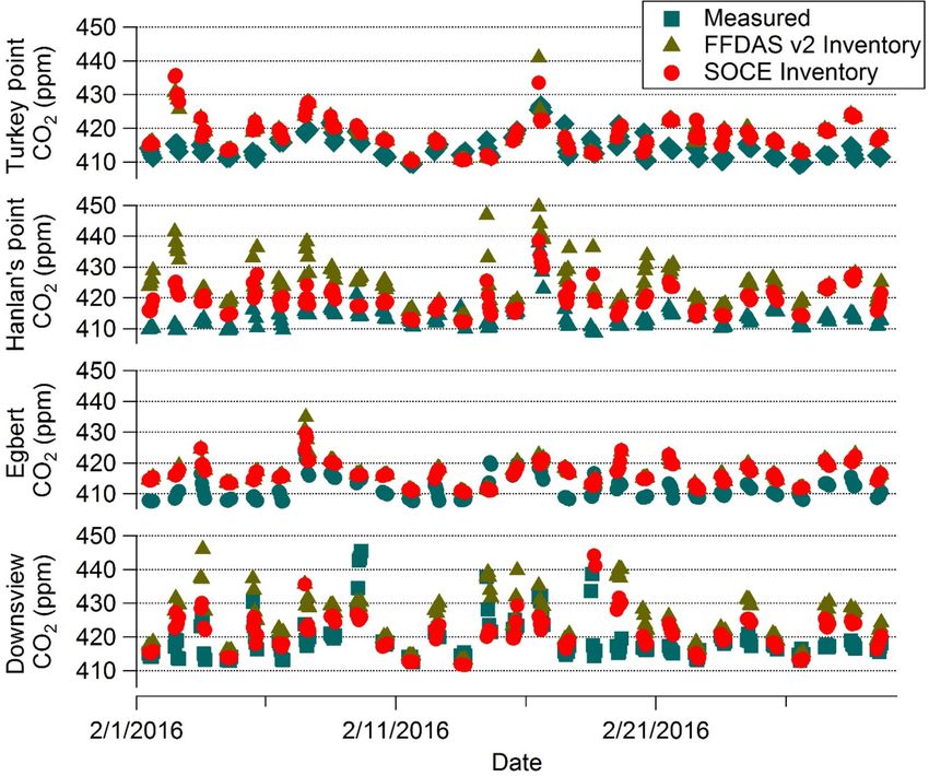
3.3 Preliminary analyses using the SOCE, FFDAS v2 and TAO are situated just north and south of downtown
and EDGAR v4.2 inventories with FLEXPART Toronto, respectively). Observed gradients ranged from +20
to −10 ppm. Figure S3 displays the measured and modelled
CO2 gradients. These results show that when the EDGAR
To investigate the impact of the different inventories on am-
v4.2 inventory was used, simulated CO2 gradients were con-
bient mixing ratios, preliminary analyses were run with foot-
sistently overestimated by ∼ 10–60 ppm relative to observa-
prints generated for every third hour of the day (e.g., 00:00,
tions. Conversely, when the SOCE inventory was used, a
03:00, 06:00, 09:00) by the FLEXPART Lagrangian particle
higher level of agreement was obtained between simulated
dispersion model (Stohl et al., 2005) driven by GEM mete-
mixing ratios and measurements; however, none of the model
orology for two sites, Downsview and TAO. Footprint areas
simulations were able to capture times when the gradient was
were multiplied by the inventory estimates to arrive at mixing
negative (CO2,TAO > CO2,Downsview ), an effect we believe to
ratio enhancements and then compared against the measured
be due to the TAO inlet being ∼ 60 m above ground level
CO2 gradient between the Downsview and TAO stations for
and surrounded by many high-rise buildings, creating canyon
the year 2014. Gradients were used to capture the CO2 mix-
flows and turbulence which are not properly accounted for
ing ratios in the downtown core of the city (since Downsview
Atmos. Chem. Phys., 18, 3387–3401, 2018 www.atmos-chem-phys.net/18/3387/2018/S. C. Pugliese et al.: High-resolution quantification of atmospheric CO2 mixing ratios 3395
FFDAS v2 domain tota l: EDGAR v4.2 domain total: SOCE domain total:
8 8 -1
1.1x10 tonne year -1 1.4x10 tonne year 9.5x10⁷ tonne year -1
(a) (b) (c)
) )
)
)
)
1 2 3 4 5 6 7
log10(tonne CO2 /year/grid cell )
Figure 3. Comparison of spatial distribution of annual CO2 emis-
sions inventories for the black-box area (shown in Fig. 2a) at
0.1◦ × 0.1◦ resolution. Panel (a) shows the FFDAS v2 inventory
estimate, panel (b) shows the EDGAR v4.2 inventory estimate, and
panel (c) shows the SOCE inventory estimate. Domain totals are
shown on top of each panel and locations of in situ measurements
of CO2 for three stations in the Southern Ontario Greenhouse Gas
Network are shown in panel (a) (Downsview is a square, Hanlan’s Figure 4. Time series of measured (blue) and modelled February
Point is a triangle, TAO is a pentagon). The other two stations, Eg- afternoon (12:00–16:00 EST) CO2 mixing ratios for the four sites
bert and Turkey Point, are located outside this area. used in this study. The red and gold markers are the modelled mix-
ing ratios when using the SOCE CO2 inventory and the FFDAS v2
inventory, respectively.
in GEM at this resolution. These factors contributed to the
decommissioning of TAO in January 2016. The poor perfor-
mance of our model system when using the EDGAR v4.2 Meteorological Satellite Program Operational Linescan Sys-
inventory to simulate CO2 mixing ratios was also found by a tem (DMSP-OLS).
study quantifying on-road CO2 emissions in Massachusetts, Beyond the differences in methodology for estimating and
USA (Gately et al., 2013). In this study, EDGAR emission allocating emissions, it is important to note that the emis-
estimates were found to be significantly larger than any other sions reported in Table 2 by the FFDAS v2, SOCE, and
inventory by as much as 9.3 million tons, or > 33 %. The dif- EDGAR v4.2 inventories also fundamentally differ in time
ference in estimates between the EDGAR v4.2 and the SOCE period quantified. The emissions reported for both FFDAS v2
inventories is likely explained by their underlying differences and the SOCE are based on emissions from 3 winter months
in methodology. Being a global product and not specifically (January–March 2010) extrapolated for the entire year. How-
designed for mesoscale applications, the EDGAR v4.2 in- ever, emissions from EDGAR v4.2 are annual averages of all
ventory estimates CO2 emissions based on country-specific 12 months of 2010. Since CO2 emissions in the GTA are
activity data and emission factors, but the spatial proxies higher in the winter months relative to the summer months
used to disaggregate the data are not always optimal. A study because of increased building and home heating, it is likely
performed by McDonald et al. (2014) showed that the use that the average annual estimates of SOCE and FFDAS v2
of road density as a spatial proxy for vehicle emissions in are slightly overestimated. This does not affect the relative
EDGAR v4.2 causes an overestimation of emissions in popu- agreement between SOCE and FFDAS v2 but it does further
lation centres (McDonald et al., 2014). Given the much larger increase the divergence between the EDGAR v4.2 and SOCE
emission estimates for on-road CO2 from EDGAR v4.2 (Ta- and FFDAS v2 inventories. Following this and the improved
ble 2), this also seems to be an issue in the GTA. Based on agreement with observations, the FFDAS v2 inventory was
this large discrepancy, the EDGAR v4.2 inventory was not used with the SOCE inventory for all subsequent modelling
further used in this study and we focussed on the inventories analyses.
developed for regional-scale studies.
When similar preliminary analyses were run with FLEX- 3.4 Simulation of CO2 mixing ratios in the Greater
PART footprints using the FFDAS v2 inventory, Fig. S3, Toronto Area
good agreement was observed with CO2 gradients measured
between the Downsview and TAO stations. We are confident We used the GEM-MACH chemistry–transport model and
that the enhanced measurement agreement between the FF- the SOCE and FFDAS v2 inventories to simulate hourly CO2
DAS v2 and SOCE relative to EDGAR v4.2 is due to im- mixing ratios in the PanAm domain. The model framework
proved methodology; spatial allocation of emissions in FF- was evaluated for a continuous 3-month period, January–
DAS v2 is achieved through the use of satellite observations March 2016, using four sampling locations in the GTA
of nightlights from human settlements from the US Defense (Fig. 1; note that measurements for the Hanlan’s Point site
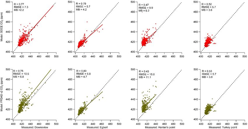
www.atmos-chem-phys.net/18/3387/2018/ Atmos. Chem. Phys., 18, 3387–3401, 20183396 S. C. Pugliese et al.: High-resolution quantification of atmospheric CO2 mixing ratios were not available until 14 January 2016). Figure 4 displays relative to measurements; however, similar to the Downsview afternoon (12:00–16:00 EST) measured and simulated CO2 site, the FFDAS v2 simulated profile has a larger difference mixing ratios produced with the SOCE and FFDAS v2 inven- of ∼ 10 ppm CO2 . At both the Egbert and Turkey Point sites, tories for the two emissions scenarios described in Sect. 2.3 the use of both inventories similarly overestimates the diur- for the month of February (Figs. S4 and S5 show the same nal pattern of CO2 mixing ratios by ∼ 3–5 ppm, again likely figure for other months). We chose to present only afternoon a result of the similarities of these two inventories at these data as this is the time of day when the mixed layer is likely sites (Fig. S1). At all four sites, it is possible that some of to be the most well-developed; nighttime and morning data the biases that are observed in simulated CO2 mixing ratios showed largest variations in observations as a result of the may arise from inaccuracies in the boundary CO2 provided shallow boundary layer causing surface emissions to accu- by MACC; this aspect was not, however, further explored in mulate within the lowest atmospheric layers (Breon et al., this study. 2015; Chan et al., 2008; Gerbig et al., 2008). During the night, atmospheric mixing ratios are most sensitive to verti- 3.5 Quantifying model–measurement agreement cal mixing, an atmospheric process that is difficult to model for stable boundary layers. Figure 6 shows scatter plots of afternoon (12:00–16:00 EST) The time series comparisons at all four sites demonstrate modelled versus measured CO2 mixing ratios from January the model’s general ability to capture variability in observa- to March 2016 at the four sites used in this study. The top tions of CO2 , albeit with better skill for the Downsview and row shows the correlation between measured and modelled Egbert sites (this is particularly clear when we look at model– mixing ratios using the SOCE inventory and the bottom row measurement difference plots; Fig. S6). The model is able to shows the correlation using the FFDAS v2 inventory. It is im- capture many extreme events of mixing ratio increases and mediately clear that there is a stronger model–measurement decreases, such as 11–14 February 2016 at the Downsview correlation at the Downsview and Egbert sites (R > 0.75) site; however, some short time periods are poorly simulated, relative to that of Hanlan’s Point or Turkey Point (R < 0.53). such as 21–23 January 2016 at Hanlan’s Point, when the The difficulty with accurately simulating CO2 mixing ra- model significantly overestimated measured CO2 . Generally, tios at Hanlan’s Point and Turkey Point may arise from their mixing ratios simulated by the FFDAS v2 inventory are simi- proximity to shorelines, Hanlan’s Point to Lake Ontario, and lar or larger than those produced when the SOCE inventory is Turkey Point to Lake Erie (see Fig. 1). Differential heating of used, with differences most noticeable at the Downsview and land versus water near these lakes creates pressure gradients Hanlan’s Point sites. This was expected as the difference plot driving unique circulation patterns (Burrows, 1991; Sills et shown in Fig. S1 reveals that the SOCE and FFDAS v2 in- al., 2011). These circulation patterns are difficult for models ventories diverge the most in the GTA (where the Downsview to capture and therefore may contribute to the relatively poor and Hanlan’s Point sites are located) and are more similar in correlation observed at Hanlan’s Point and Turkey Point. rural areas (where the Turkey Point and Egbert sites are lo- It is also clear from Fig. 6 that simulating CO2 mixing cated). ratios at the Egbert and Turkey Point sites using either the Measured CO2 mixing ratios have a typical diurnal pat- FFDAS v2 or the SOCE inventory results in similar perfor- tern, in which mixing ratios are higher at night and lower mance, likely because the emissions estimated by the two during the day, despite higher emissions during the day. This inventories are similar in the vicinity of these two rural results from the daily cycle of the mixed layer, which is shal- sites (see also Fig. 5). However, at both the Downsview and low at night due to thermal stratification and deepens during Hanlan’s Point sites, using the SOCE inventory provided a the day due to solar heating of the surface. Figure 5 displays slightly higher correlation and reduced root-mean-square er- the measured and modelled mean diurnal profile of CO2 at ror (RMSE) and mean bias relative to using the FFDAS v2 the four sites in our network using data from January to inventory. The improvement by using the SOCE inventory is March 2016 (note difference in y-axis scale for urban vs. ru- likely a result of both the improved spatial resolution (2.5 km ral sites). At all four sites, the shapes of the modelled and vs. 10 km), and therefore more accurate allocation of emis- measured mixing ratios throughout the day agree very well, sions to grid cells and also a better estimation of emission suggesting that the GEM meteorology in our framework is magnitudes, as large differences are shown in Figs. 3 and S1. capturing the diurnal variation in emissions and the boundary layer evolution. At the Downsview site, there is a very strong 3.6 Sectoral contributions to simulated CO2 mixing agreement between the modelled and measured diurnal pro- ratios files when using the SOCE inventory, whereas the FFDAS v2 simulated profile largely overestimates mixing ratios, partic- One of the major advantages of the SOCE inventory over ularly at nighttime. This is consistent with the FFDAS inven- the FFDAS v2 inventory is the availability of sectoral emis- tory having larger emissions than the SOCE inventory during sion estimates. Figure 7 displays the sectoral percent con- the night (Fig. S2). At the Hanlan’s Point site, a difference tributions to diurnal CO2 mixing ratio enhancements (calcu- of ∼ 5 ppm CO2 is observed when using the SOCE inventory lated as local CO2 mixing ratios above the MACC-estimated Atmos. Chem. Phys., 18, 3387–3401, 2018 www.atmos-chem-phys.net/18/3387/2018/
S. C. Pugliese et al.: High-resolution quantification of atmospheric CO2 mixing ratios                                                3397

Figure 5. Time series of mean measured (blue) and modelled diurnal CO2 mixing ratios at the four sites considered in this study for
January–March 2016. The red and gold markers are the modelled diurnal mixing ratios when using the SOCE CO2 inventory and the FFDAS
v2 inventory, respectively. Note the difference in scale for urban and rural sites. Error bars represent standard error of the mean.

Figure 6. Scatter plot of the modelled and measured afternoon (12:00–16:00 EST) CO2 mixing ratios from January to March 2016 at the
four monitoring stations used in this study. The top and bottom panels show measurement–model correlation when the SOCE inventory and
the FFDAS v2 inventory were used, respectively. The model vs. measurement correlation coefficient (R), root-mean-square error (RMSE),
and mean bias (MB) (unit: ppm) are provided within each panel. Solid lines are the standard major axis regression lines and dashed lines are
1 : 1 lines shown for reference.

www.atmos-chem-phys.net/18/3387/2018/                                                      Atmos. Chem. Phys., 18, 3387–3401, 2018
3398                                  S. C. Pugliese et al.: High-resolution quantification of atmospheric CO2 mixing ratios

                                                                     mented by running simulations with additional tracers, such
                                                                     as CO, nitrogen oxides (NOx ), or stable carbon isotopes (12 C
                                                                     and 13 C) to gain further insight.

                                                                     4   Conclusions

                                                                     We presented the SOCE inventory for Southern Ontario and
                                                                     the GTA, the first, to our knowledge, high-resolution CO2 in-
                                                                     ventory for Southern Ontario and for a Canadian metropoli-
                                                                     tan region. The SOCE inventory provides CO2 emissions es-
                                                                     timates at 2.5 km × 2.5 km spatial and hourly temporal reso-
                                                                     lution for seven sectors: area, residential natural-gas combus-
Figure 7. Modelled sectoral percent contributions to diurnal local   tion, commercial natural-gas combustion, point, marine, on-
CO2 enhancement for February 2016 at Downsview averaged by           road, and off-road. When compared against two existing CO2
day of week. Note: area = area + residential natural-gas combus-     inventories available for Southern Ontario, the EDGAR v4.2
tion + commercial natural-gas combustion. (Time zone is EST).        and the FFDAS v2 inventories, using FLEXPART footprints,
                                                                     the SOCE inventory had improved model–measurement
                                                                     agreement; FFDAS v2 agreed well with in situ measure-
                                                                     ments, but the EDGAR v4.2 inventory systematically overes-
background) for the Downsview station in February 2016
                                                                     timated mixing ratios. We developed a model framework us-
averaged by the day of week (Figs. S7 and S8 displays the
                                                                     ing the GEM-MACH chemistry–transport model on a high-
same for other months). This figure clearly demonstrates the
                                                                     resolution 2.5 km × 2.5 km grid coupled to the SOCE and
importance of area emissions (defined here as the sum of
                                                                     FFDAS v2 inventories for anthropogenic CO2 emissions
the area + residential natural-gas combustion + commer-
                                                                     and C-TESSEL for biogenic CO2 fluxes. We compared out-
cial natural-gas combustion) to simulated CO2 mixing ratios,
                                                                     put simulations to observations made at four stations across
reaching ∼ 80 % contribution in the early morning and late
                                                                     Southern Ontario and for 3 winter months, January–March
evening, consistent with times when emissions from home
                                                                     2016. Model–measurement agreement was strong in the af-
heating are the dominant source of CO2 . Contributions from
                                                                     ternoon using both anthropogenic inventories, particularly
area emissions decrease to ∼ 35 % midday, which coincides
                                                                     at the Downsview and Egbert sites. Difficulty in capturing
with when emissions from other sources, such as on-road,
                                                                     mixing ratios at the Hanlan’s Point and Turkey Point sites
gain importance. In the midday, emissions from the on-road
                                                                     was hypothesized to be a result of their close proximity to
sector can contribute ∼ 50 %, which is consistent with trans-
                                                                     shorelines (Lake Ontario and Lake Erie, respectively) and
portation patterns of the times when the population is trav-
                                                                     the model’s inability to capture the unique circulation pat-
elling to and from work and other activities. The relative
                                                                     terns that occur in those environments. Generally, across all
contributions to CO2 mixing ratios from point-source emis-
                                                                     stations and months, simulations using the SOCE inventory
sions are quite variable during the course of a day and week,
                                                                     resulted in higher model–measurement agreement than those
but they generally seem to increase in the early morning
                                                                     using the FFDAS v2 inventory, quantified using R, RMSE,
and evening and can contribute a significant portion of total
                                                                     and mean bias. In addition to improved agreement, the pri-
CO2 emissions (up to ∼ 20 %). Figure 7 indicates that bio-
                                                                     mary advantage of the SOCE inventory over the FFDAS v2
genic sources of CO2 play a negligible role during January–
                                                                     inventory is the sectoral breakdown of emissions; using av-
March in the GTA (the biogenic line is not visible because
                                                                     erage day-of-week diurnal mixing ratio enhancements, we
it is located on the zero line underneath the marine line).
                                                                     were able to demonstrate that emissions from area sources
Recent studies, however, have shown the importance of the
                                                                     can contribute > 80 % of CO2 mixing ratio enhancements in
biospheric contribution (up to ∼ 132–308 g CO2 km−2 s−1 )
                                                                     the early morning and evening with on-road sources con-
to measured CO2 in urban environments during the grow-
                                                                     tributing > 50 % midday. The applications of the SOCE in-
ing season (Decina et al., 2016). Therefore, this finding sup-
                                                                     ventory will likely show future utility in understanding the
ports the importance of modelling CO2 in the wintertime in
                                                                     impacts of CO2 reduction efforts in Southern Ontario and
cities like the GTA to avoid complications associated with
                                                                     identify target areas requiring further improvement.
biospheric contributions. The new ability to understand the
sectoral contributions to CO2 mixing ratios in the GTA and
Southern Ontario has implications from a policy perspective;         Data availability. The data can be found in Pugliese (2018;
with recent initiatives to curb CO2 emissions, understanding         doi:10.5683/SP/GOQGHD).
from which sector the CO2 is being emitted could be useful to
assess how effective applied mitigation efforts have been or
where to target future efforts. These efforts could be comple-

Atmos. Chem. Phys., 18, 3387–3401, 2018                                               www.atmos-chem-phys.net/18/3387/2018/
You can also read