Structure and drivers of ocean mixing north of Svalbard in summer and fall 2018
←
→
Page content transcription
If your browser does not render page correctly, please read the page content below
Ocean Sci., 17, 365–381, 2021
https://doi.org/10.5194/os-17-365-2021
© Author(s) 2021. This work is distributed under
the Creative Commons Attribution 4.0 License.

Structure and drivers of ocean mixing north of Svalbard
in summer and fall 2018
Zoe Koenig1,2 , Eivind H. Kolås1 , and Ilker Fer1
1 Geophysical  Institute, University of Bergen and Bjerknes Center for Climate Research, Bergen, Norway
2 Norwegian   Polar Institute, Tromsø, Norway

Correspondence: Zoe Koenig (zoe.koenig@uib.no)

Received: 24 July 2020 – Discussion started: 3 August 2020
Revised: 20 November 2020 – Accepted: 18 January 2021 – Published: 19 February 2021

Abstract. The Arctic Ocean is a major sink for heat and salt      umn vertically. Understanding the drivers of turbulence and
for the global ocean. Ocean mixing contributes to this sink by    the nonlinear pathways for the energy to turbulence in the
mixing the Atlantic- and Pacific-origin waters with surround-     Arctic Ocean will help improve the description and repre-
ing waters. We investigate the drivers of ocean mixing north      sentation of the rapidly changing Arctic climate system.
of Svalbard, in the Atlantic sector of the Arctic, based on
observations collected during two research cruises in sum-
mer and fall 2018. Estimates of vertical turbulent heat flux
                                                                  1   Introduction
from the Atlantic Water layer up to the mixed layer reach
30 W m−2 in the core of the boundary current, and average         The Arctic Ocean is a sink for salt and heat. Relatively
to 8 W m−2 , accounting for ∼ 1 % of the total heat loss of       warm and salty Atlantic waters enter the Arctic Ocean via
the Atlantic layer in the region. In the mixed layer, there is    Fram Strait and the Barents Sea through-flow, and colder
a nonlinear relation between the layer-integrated dissipation     and fresher Arctic waters exit flowing east of Greenland
and wind energy input; convection was active at a few sta-        through the East Greenland Current. Annual average water
tions and was responsible for enhanced turbulence compared        mass transformation in the Arctic is about −0.62 ± 0.23 in
to what was expected from the wind stress alone. Summer           salinity and −3.74±0.76 ◦ C in temperature (Tsubouchi et al.,
melting of sea ice reduces the temperature, salinity and depth    2018). With the rapid and large sea ice decline, the Arctic
of the mixed layer and increases salt and buoyancy fluxes at      Ocean is particularly vulnerable to climate change. In the
the base of the mixed layer. Deeper in the water column and       near future we will enter a new regime, in which the inte-
near the seabed, tidal forcing is a major source of turbulence:   rior Arctic Ocean is entirely ice-free in summer and sea ice
diapycnal diffusivity in the bottom 250 m of the water col-       is thinner and more mobile in winter (Guarino et al., 2020),
umn is enhanced during strong tidal currents, reaching on av-     which will have vast implications for the Arctic Ocean cir-
erage 10−3 m2 s−1 . The average profile of diffusivity decays     culation, the marine ecosystems it supports and the larger-
with distance from the seabed with an e-folding scale of 22 m     scale climate (Timmermans and Marshall, 2020). The heat
compared to 18 m in conditions with weaker tidal currents.        contained in the Atlantic- and Pacific-origin waters has the
A nonlinear relation is inferred between the depth-integrated     potential to melt the entire sea ice if it reaches the surface
dissipation in the bottom 250 m of the water column and the       (Maykut and Untersteiner, 1971). The estimated mean Arc-
tidally driven bottom drag and is used to estimate the bottom     tic Ocean surface heat flux necessary to keep the sea ice
dissipation along the continental slope of the Eurasian Basin.    thickness at equilibrium is 2 W m−2 (Maykut and McPhee,
Computation of an inverse Froude number suggests that non-        1995), yet observations indicate mean surface heat fluxes of
linear internal waves forced by the diurnal tidal currents (K1    3.5 W m−2 (Krishfield and Perovich, 2005). To assess the
constituent) can develop north of Svalbard and in the Laptev      evolution of the sea ice, the oceanic heat in the Arctic must
and Kara seas, with the potential to mix the entire water col-    be monitored and understood.

Published by Copernicus Publications on behalf of the European Geosciences Union.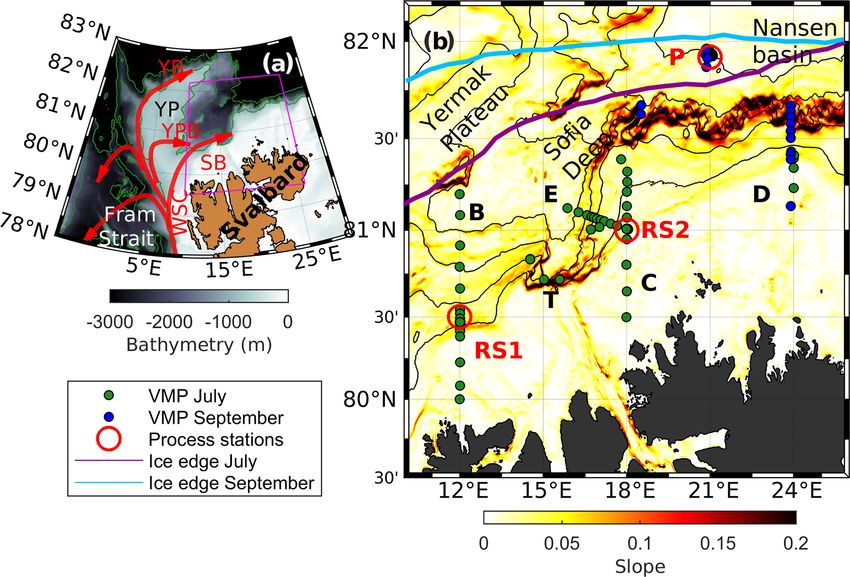
366                                                                          Z. Koenig et al.: Ocean mixing north of Svalbard

   Atlantic Water is a major component of the Arctic Ocean
heat budget, with particular influence in the Atlantic sec-
tor. An important player in the transformation of the At-
lantic Water is vertical mixing. The central Arctic is rela-
tively quiescent (Fer, 2009; Lincoln et al., 2016). Microstruc-
ture measurements indicate turbulent kinetic energy dissipa-
tion in the halocline of the deep basins to be around 10−10 to
10−9 W kg−1 (Fer, 2009; Lincoln et al., 2016; Rippeth et al.,
2015). The dissipation rates are estimated to be several or-
ders of magnitude larger on the ocean margins than over the
abyssal plain (Padman and Dillon, 1991; Lenn et al., 2011;
Rippeth et al., 2015; Fer et al., 2015).
   North of Svalbard is a location with enhanced mixing. It is
also a key region for the Arctic Ocean heat and salt budget,
as it is the gateway for Fram Strait inflow of Atlantic Wa-
ter. The circulation of Atlantic Water here is complex, with        Figure 1. (a) Circulation pattern of Atlantic Water around Svalbard,
                                                                    with the West Spitsbergen Current (WSC), the Svalbard Branch
several recirculations in Fram Strait and three main inflow
                                                                    (SB), the Yermak Branch (YB) and the Yermak Pass Branch (YPB).
branches including the Yermak Branch (YB; Cokelet et al.,           Bathymetry is from the International Bathymetric Chart of the Arc-
2008), the Yermak Pass Branch (YPB; Koenig et al., 2017;            tic Ocean, IBCAO-v3 (Jakobsson et al., 2012). (b) Close-up of the
Crews et al., 2019; Menze et al., 2019) and the Svalbard            magenta box in (a). Station locations (July, green dots; September,
Branch (SB; Cokelet et al., 2008), all originating from the         blue dots), sections (B, C, D and E) and process stations (red circles
West Spitsbergen Current (WSC) (Fig. 1a). As the Atlantic           marked RS1, RS2 and P) are shown. The slope steepness calcu-
Water flows eastward, it deepens and gets colder and fresher        lated from IBCAO-v3 is color-coded in the background. Isobaths
due to mixing with the surrounding waters.                          are drawn every 1000 m in (a) and 500 m in (b). Purple/light blue
   Cooling and freshening of the Atlantic Water north of            lines are the averaged sea ice edge defined as the 15 % ice concen-
Svalbard result from different processes. Along the slope           tration over the summer and fall cruise, respectively.
north of Svalbard, eddies are shed from the Atlantic Water
Boundary Current (Våge et al., 2016; Crews et al., 2018),
transporting 0.16 Sv (1 Sv = 106 m3 s−1 ) of Atlantic Water         Atlantic layer reaching the surface (Duarte et al., 2020) and
and 1.0 TW (1 TW = 1012 W) away from the boundary cur-              is associated with the Atlantification of the Eurasian Basin
rent. Large vertical turbulent fluxes can occur in localized        and of the Barents Sea (Polyakov et al., 2017; Årthun et al.,
regions. Strong tidal currents over bathymetric slopes and          2012). In the Eurasian Basin, the upward oceanic heat flux
rough topography generate internal waves which are a major          towards the mixed layer has increased from 3–4 W m−2 in
source of energy for increased turbulence dissipation rates         2007–2008 to more than 10 W m−2 in 2016–2018 (Polyakov
(Padman et al., 1992; Rippeth et al., 2017; Fer et al., 2020b).     et al., 2020). This process is called the ice–ocean heat feed-
Rippeth et al. (2015) showed that the Yermak Plateau is a hot       back as the increased ocean heat flux to the sea surface re-
spot for tidal mixing. Fer et al. (2015) suggested that in this     duces ice thickness and increases its mobility, increasing
region, almost the entire volume-integrated dissipation can         atmospheric momentum flux into the ocean and reducing
be attributed to the loss of baroclinic tidal energy converted      the damping of surface-intensified baroclinic tides (Polyakov
locally from the surface tides. In the Nansen Basin north of        et al., 2020). Mixing north of Svalbard is of particular interest
Svalbard, turbulence in the upper layer influences the sea ice      to understand the Atlantification as it contributes to the cool-
cover. Peterson et al. (2017) found an average winter ocean-        ing and freshening of the Atlantic Water entering the Arc-
to-ice heat flux of around 1.4 W m−2 , with episodic local up-      tic Ocean. The reduced ice cover over the continental slope
welling events and proximity to Atlantic Water pathways in-         north of Svalbard can be seen as a precursor of the entire
creasing the heat fluxes by 1 order of magnitude. Meyer et al.      Eurasian Basin and the processes therein. Indeed, Polyakov
(2017) presented 6 months of turbulence data collected from         et al. (2020) documented an eastward lateral propagation of
January to June 2015 during the N-ICE2015 campaign. The             the so-called Atlantification, with a lag of about 2 years be-
combination of storms and shallow Atlantic Water leads to           tween the Barents Sea and the eastern Eurasian Basin. There-
the highest heat flux rates observed: ice–ocean interface heat      fore, detailed observations of the ocean dynamics north of
fluxes averaged 100 W m−2 during peak events.                       Svalbard are needed to evaluate the active processes modify-
   In the last decade, ice-free regions have been observed          ing the Atlantic Water layer in a changing Arctic, and their
along the path of the Atlantic Water, in the Barents Sea first      potential influence on the sea ice.
and then in the Eurasian Arctic Ocean, with warm and saline            In this study we present observations of ocean turbulence
water extending up to the surface (Årthun et al., 2012; Ivanov      north of Svalbard collected in summer and fall 2018 and fo-
et al., 2016). The lack of sea ice is mainly due to heat from the   cus on mechanisms which lead to turbulence in the different

Ocean Sci., 17, 365–381, 2021                                                             https://doi.org/10.5194/os-17-365-2021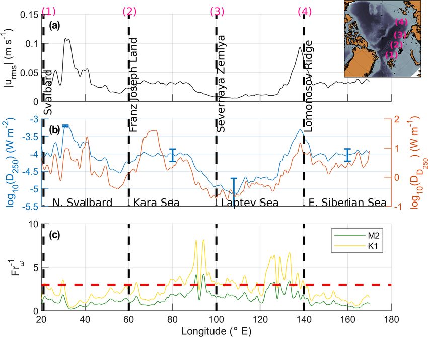
Z. Koenig et al.: Ocean mixing north of Svalbard                                                                              367

layers of the water column. Two main sources of ocean mix-        individual spectra and individual dissipation rate profiles
ing are investigated: the wind and the tidal forcing. Turbu-      from the two shear probes. We averaged estimates from both
lence production by background shear will not be addressed        probes, except when their ratio exceeded 10, for example as
in this study as the vertical resolution (8 m) of the current     a result of plankton hitting a sensor, and the lowest estimate
data collected during the cruises is not sufficient to resolve    was chosen. The noise level of the dissipation rate measured
shear instabilities.                                              by the VMP is about (2–3) × 10−10 W kg−1 . The tempera-
                                                                  ture and salinity data from the VMP were compared against
                                                                  the ship’s SBE CTD (conductivity, temperature, depth) pro-
2     Data and methods                                            files. A good agreement was observed and no correction was
                                                                  made. Dissipation measurements from the upper 15 m were
Data were collected in 2018, during two cruises that took
                                                                  excluded because of the disturbance from the ship’s keel
place north of Svalbard as a part of the Nansen Legacy
                                                                  and the profiler’s adjustment to free fall. The vertically in-
Project. The summer cruise was on R/V Kristine Bonnevie
                                                                  tegrated dissipation rate over a layer h (surface mixed layer
from 27 June to 10 July 2018 (Fer et al., 2019), while the fall
                                                                  or near-bottom   layer in the following sections) is defined
cruise was on the ice-class R/V Kronprins Haakon from 12
                                                                  as Dh = ρ0 h (z)dz (in W m−2 ) where ρ0 = 1027 kg m−3 is
                                                                              R
to 24 September 2018 (Fer et al., 2020a). During the cruises,
                                                                  the seawater reference density.
several sections were repeated north of Svalbard across the
                                                                     We estimated the turbulent heat flux FH from
continental slope, and three stations (two in July and one in
September) were occupied for about 24 h to study mixing                           ∂2
processes (Fig. 1b). Turbulence profiles were collected dur-      FH = −ρ0 Cp κ      ,                                        (2)
                                                                                  ∂z
ing both cruises (185 profiles in 9 d in July and 43 in 5 d in
September) using a Vertical Microstructure Profiler (VMP).        where Cp = 3991.9 J kg−1 K−1 is the specific heat of seawa-
We calculated the Conservative Temperature (2) and Ab-            ter, 2 is the background temperature and κ is the diapycnal
solute Salinity (SA ) using the International Thermodynamic       eddy diffusivity. We thus assume that turbulence diffuses the
Equations of SeaWater (TEOS-10) (McDougall and Barker,            fine-scale temperature gradient at the same rate as the density
2011).                                                            gradient. The sign convention is that positive heat fluxes are
                                                                  directed upward in the water column.
2.1    Vertical Microstructure Profiler (VMP)                        We expressed the diapycnal diffusivity κ following Bouf-
                                                                  fard and Boegman (2013), where three states (energetic, tran-
We used a 2000 m rated VMP manufactured by Rockland               sitional and buoyancy-controlled) are defined depending on
Scientific, Canada (RSI). The VMP is a loosely tethered pro-      the buoyancy Reynolds number, Reb = νN 2 . In the transi-
filer with a nominal fall speed of 0.6 m s−1 . The profiler was   tional range (8.5 < Reb < 400), calculation of κ is identical
equipped with pumped Sea-Bird Scientific (SBE) conductiv-         to Osborn (1980), using the canonical mixing coefficient of
ity and temperature sensors, a pressure sensor, airfoil veloc-    0.2 (Gregg et al., 2018); however, in the energetic regime
ity shear probes, one high-resolution temperature sensor, one     the latter is an overestimate. In our dataset, 80 % of the es-
high-resolution micro-conductivity sensor and three orthog-       timates are in the transitional regime. To compute κ, the
onal accelerometers. The microstructure data were processed       buoyancy frequency or Brunt–Väisälä frequency, N, was ap-
using the routines provided by RSI (ODAS v4.01). Assuming         proximated using N 2 = − ρg0 ∂σ  0
                                                                                                 ∂z , where g is the gravitational
isotropic turbulence, the dissipation rate of turbulent kinetic   acceleration and σ0 is the potential density anomaly refer-
energy per unit mass, , can be expressed as                      enced to surface pressure. Background vertical gradients (for
             2                                                  temperature, salinity and density) were taken over a 10 m
         ∂u                                                       length scale. To prevent spuriously large values of κ as N ap-
 = 7.5ν           ,                                       (1)
         ∂z                                                       proaches neutral stratification, segments with buoyancy fre-
                                                                  quency below a noise level of N 2 = 10−7 s−2 were excluded.
where ν is the kinematic viscosity equal to about 1.6 ×              We also computed the salt flux FS and the buoyancy flux
10−6 m2 s−1 in these temperatures, the overbar denotes av-        FB :
eraging in time and ∂u/∂z is the small-scale shear of one
horizontal velocity component u. Dissipation rates were cal-               ∂SA
                                                                  FS = −ρ0 κ   ,                                              (3)
culated from the shear variance obtained by integrating the                 ∂z
shear vertical wavenumber spectra in a wavenumber range           FB = −g(βFS − αFH ),                                        (4)
that is relatively unaffected by noise and corrected for the
variance in the unresolved portions of the spectrum us-           where α and β are respectively the thermal expansion and
ing an empirical model (Nasmyth, 1970). The shear spectra         salinity contraction coefficients, g is the gravitational con-
were computed using 1 s Fourier transform length and half-        stant, and the positive fluxes are directed upward.
overlapping 4 s segments. We quality-screened the resulting          In the rest of the study, sets of three to four consecutive
values by inspecting the instrument accelerometer records,        repeat profiles at the process stations are averaged to avoid

https://doi.org/10.5194/os-17-365-2021                                                          Ocean Sci., 17, 365–381, 2021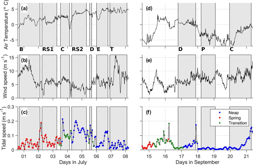
368                                                                        Z. Koenig et al.: Ocean mixing north of Svalbard

any bias toward these stations. Table 1 lists two numbers of       ter the winch broke, resulting in fewer profiles (section D,
“profiles”: the total number of casts performed (number of         process study P and the outer deep stations at section C).
profiles) and the number of profiles used in analyses (n) af-         In July, the Yermak Plateau was covered by sea ice, and the
ter batch-averaging of consecutive repeat profiles. In the rest    ice edge was close to the continental slope north of Svalbard
of the study, we always refer to the number of profiles after      (Fig. 1), limiting the station coverage (e.g., section D could
batch-averaging (in Figs. 4 and 7).                                not be completed). We note that the sea ice encountered in
                                                                   July was closer to the continental slope at 24 ◦ E than what
2.2    Other datasets                                              is suggested by the sea ice edge from satellite, defined here
                                                                   as 15 % sea ice concentration. In September, the sea ice edge
We used the profiles collected from the ship’s CTD system          was ∼ 30 to 50 km further north, and the continental slope
(Sea-Bird Scientific, SBE 911plus on both cruises) to check        was entirely free of ice, which can facilitate enhanced wind
the temperature and salinity from the VMP. CTD data were           energy input to the oceanic near-inertial currents (Rainville
processed using the standard SBE post-processing software,         and Woodgate, 2009).
and salinity values were corrected against water sample anal-         Air temperature differs between the two cruises: while
yses. Pressure, temperature and practical salinity data are ac-    it was mainly positive in July, the temperature dropped to
curate to ±0.5 dbar, ±2 × 10⁻³ ◦ C, and ±3 × 10⁻³ , respec-        −10 ◦ C in September (Fig. 2a and d) near the sea ice edge.
tively.                                                            Over the two cruises, wind was moderate, peaking only for
   The wind speed, direction and surface air temperature           half a day to 15 m s−1 on 7 July (Fig. 2b). In September, the
(Fig. 2) were recorded every minute during the cruises from        average wind speed was 8 m s−1 with no specific events. Dur-
the ship’s weather station. The wind energy flux from the at-      ing the cruise in September, surface gravity waves were es-
mosphere into the ocean is estimated from the wind speed           timated using single-point ocean surface elevation data ob-
                                                 3 (Oakey and
at 10 m height (U10 ) as E10 = τ U10 = ρair Cd U10                 tained from the bow of the ship using a system that combines
Elliott, 1982), where ρair is the density of air and τ is the      an altimeter and inertial motion unit (Løken et al., 2019). The
wind stress, parameterized using a quadratic drag with a drag      significant wave height varied between 0.5 and 1.5 m with
coefficient Cd . We use the neutral drag coefficient at 10 m       mean wave periods between 2 and 6 s.
computed following Large and Pond (1981), adjusting the               Tidal currents varied significantly during the cruise de-
wind speed measured at 15 m height in July and 22 m height         pending on the location, with a maximum amplitude about
in September from the ship’s mast to 10 m.                         20 cm s−1 during RS2 from 4 to 6 July. The tidal currents
   We used Arc5km2018 (Erofeeva and Egbert, 2020), a               were stronger on the slope than in the deep basin (such as
barotropic inverse tidal model on a 5 km grid, to estimate the     during P in the Nansen Basin). In July, sections were occu-
tidal currents using the eight main constituents (M2 , S2 , N2 ,   pied during spring tides for the first 3 d and during neap tides
K2 , K1 , O1 , P1 and Q1 ) and four nonlinear components (M4 ,     for the rest of the cruise. In September, the tidal currents at
MS4 , MN2 and 2N2 ).                                               the stations were weaker and mainly during neap tides, ex-
   Bathymetric contours shown in maps are from the Inter-          cept for a short period of spring tides in the beginning of the
national Bathymetric Chart of the Arctic Ocean (IBCAO-v3)          cruise (around 15 September 2018).
(Jakobsson et al., 2012). Station depths are from the ship’s
echosounder.                                                       3.2   Hydrography
   To discuss our findings in a broader scope, we used the
global monthly isopycnal mixed-layer ocean climatology             Figure 3 shows the distribution of temperature and dissipa-
(MIMOC) at 0.5◦ resolution, which is objectively mapped            tion rate collected in sections and the process stations per-
with emphasis on data from the last decade (Schmidtko et al.,      formed during the two cruises. Temperature sections were
2013).                                                             obtained by gridding the data in 1 km horizontal and 2 m ver-
                                                                   tical grid size using linear interpolation.
                                                                      We estimate the mixed layer depth (dark green line in
3     Overview of observations                                     Fig. 3) as the depth at which the density exceeds the shallow-
                                                                   est measurement by 0.01 kg m−3 in July and by 0.03 kg m−3
3.1    Environmental context                                       in September, because of the presence of meltwater at the sur-
                                                                   face in September. The vertical gradients are large, and the
The cruises cover the summer and fall conditions, typically in     mixed layer depth is not very sensitive to the exact criterion.
open waters. Four main sections were occupied north of Sval-       An estimate of a surface layer depth (not shown) following
bard: Section B, C and E in July, and section D in Septem-         Randelhoff et al. (2017) was very similar.
ber, capturing the core of the inflowing Atlantic Water. Se-          The slope north of Svalbard is characterized by Atlantic
lected stations were occupied for 24 h to investigate mixing       Water flowing along the 800 m isobath. The Atlantic Water
processes in detail at a specific location: T, RS1, RS2 and P      is defined as water masses with 2 > 2 ◦ C and 27.7 < σ0 <
(Fig. 1b). In September, turbulence profiling terminated af-       27.97 kg m−3 following Rudels et al. (2000). The warm wa-

Ocean Sci., 17, 365–381, 2021                                                          https://doi.org/10.5194/os-17-365-2021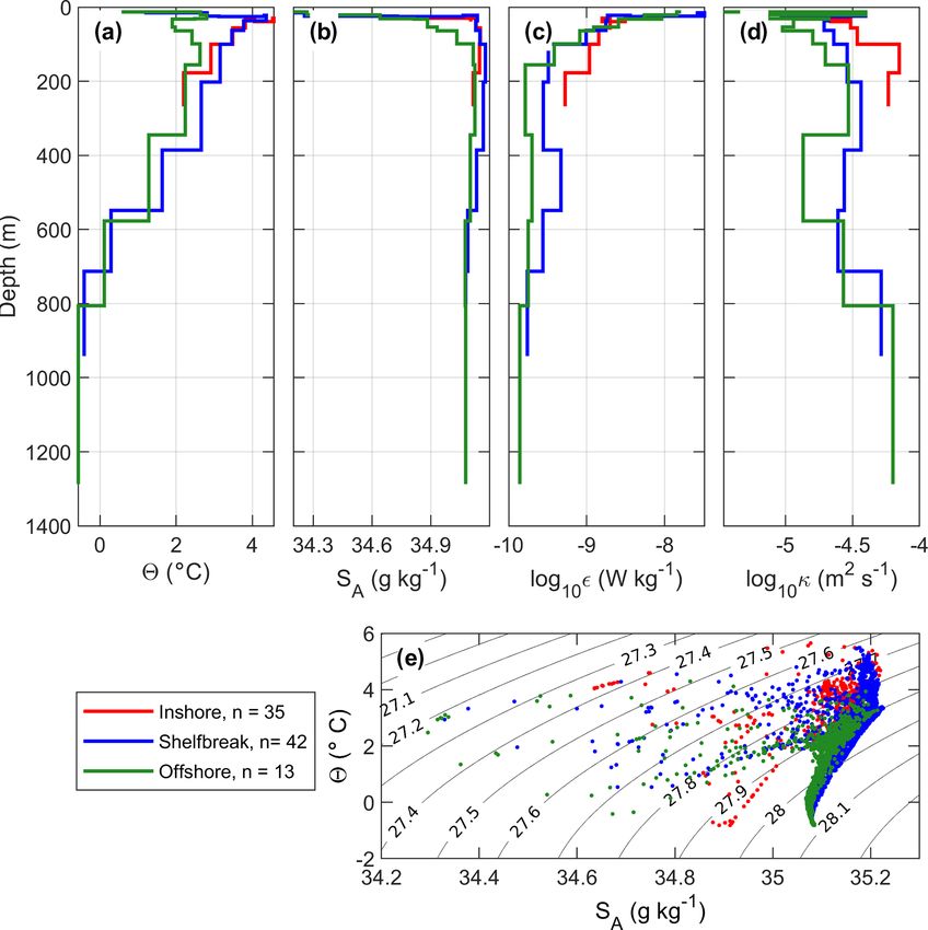
Z. Koenig et al.: Ocean mixing north of Svalbard                                                                                         369

Table 1. Overview of ocean microstructure measurements. The number of profiles used in analyses is n, after batch-averaging repeat profiles
in the process stations.

                   Start                               End                                Instrument     Number of       n
                                                                                                           profiles
                   30 June 2018, 17:30 UTC             8 July 2018, 20:00 UTC             VMP 2000              185    76
                   16 September 2018, 21:30 UTC        20 September 2018, 04:40 UTC       VMP 2000               43    14

Figure 2. Air temperature (a, d), wind speed (b, e) from the ship’s weather station and tidal current speed (c, f) from the Arc5km2018
model. Panels (a)–(c) are during the July (Summer) cruise. Panels (d)–(f) are during the September (fall) cruise. Grey shading corresponds
to the periods of turbulence measurements (sections or process stations). In (c) and (f), the tidal conditions during the time of sampling are
indicated as neap, spring tide, and the transition between the neap and spring tide with blue, red and green dots respectively.

ters observed roughly between 500 and 1100 m isobaths are                distance from the 800 m isobath, which is representative of
associated with the Atlantic Water core (section panels in               the mean location of the core of the inflowing Atlantic Wa-
Fig. 3 and blue line in Fig. 4a). Colder and fresher waters              ter (Kolås et al., 2020). The core of the Atlantic Water cur-
found offshore are Atlantic Water from Fram Strait, which                rent typically extends about 20 km onshore and offshore of
has been modified by mixing with the surrounding waters.                 the 800 m isobath (Kolås et al., 2020). However, in order to
A thorough description of the hydrography and circulation                characterize the different regions of the slope with a compa-
during the two cruises can be found in Kolås et al. (2020).              rable number of profiles in each region, we present averages
   We calculated average profiles of temperature, salinity,              −10 km inshore, within ±10 km of the 800 m isobath and
dissipation rate and diffusivity using data combined from                10 km offshore (Fig. 4).
both July and September cruises. The averaging is made in                   Averaged temperature and salinity profiles are very similar
isopycnal coordinates to account for the possible vertical dis-          at depth (below 600 m, around 0 ◦ C and 35.1 g kg−1 ; Fig. 4e),
placement of isopycnals and water masses from the slope to               and the main differences are observed in the upper 200 m.
the deep basin. Once averaged, the profiles are mapped onto              The “inshore” average profile is the warmest with a temper-
vertical coordinates using the corresponding average depth of            ature maximum of ∼ 5.5 ◦ C at around 75 m depth. The “off-
an isopycnal (Fig. 4). While this averaging is representative            shore” average profile has the coldest mixed layer (around
of the vertical structure below the mixed layer, it is probably          0 ◦ C) and the coldest core of Atlantic Water (around 2 ◦ C), a
not appropriate for the surface layer where surface stratifica-          characteristic of the hydrography in the Nansen Basin (Kolås
tion and buoyancy flux are significantly different in July and           et al., 2020).
September (see the following section for more details). The
average profiles are obtained in subsets, depending on their

https://doi.org/10.5194/os-17-365-2021                                                                    Ocean Sci., 17, 365–381, 2021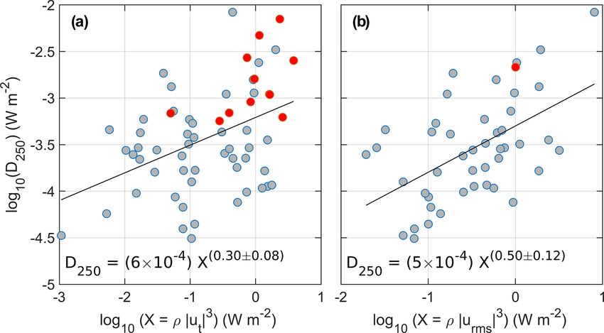
370 Z. Koenig et al.: Ocean mixing north of Svalbard
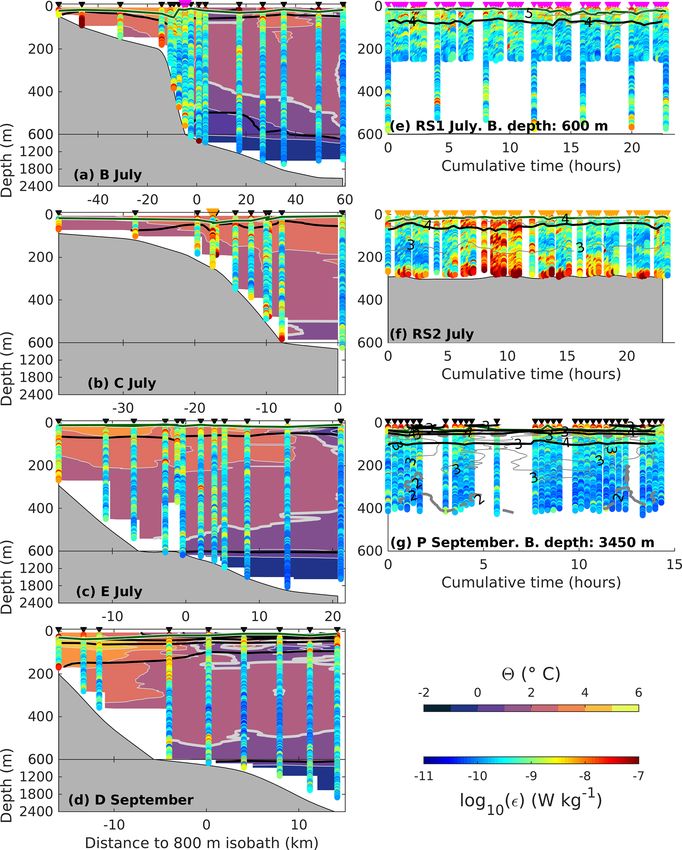
Figure 3. Overview of the main sections (a–d) and the process study stations (e–g) during the July and September cruises. In (a)–(d), back-
ground is 2, and the dissipation rate profiles () are superimposed. Note the change of vertical scale at 600 m depth. In (e)–(g), temperature
contours are shown as thin grey lines. In all panels, bold black lines are the isopycnals, and the thicker grey line is the 2 ◦ C isotherm.
Bathymetry is from the bottom depth measured at each station. Triangle markers are the time or location of the stations. In (a) and (b), the
pink and orange station markers indicate the location of the RS1 and RS2 process station, respectively, shown in (e) and (f). At station P (g),
one early VMP cast performed about 6 h before the start of the first shown profile is excluded. The horizontal axis is the distance to the 800 m
isobath in the (a)–(d) and cumulative time from the first profile in (e)–(g). The dark green line is the mixed layer depth.
3.3 Turbulence Water current (blue profiles), where the strongest currents are
observed (Kolås et al., 2020). Diffusivity is large in both the
On average, dissipation rates are the largest in the upper mixed layer and at depth close to the bottom (Fig. 4d), ex-
ocean, reaching 10−7 W kg−1 near the surface and decreas- ceeding 6 × 10⁻⁵ m2 s−1 .
ing rapidly with depth (Fig. 4c). In deeper layers, the dis- Of the microstructure measurements collected during the
sipation rates are larger inshore than offshore, decreasing cruises, the process stations RS2 and P were analyzed and re-
from 5 × 10⁻¹⁰ W kg−1 in the shallows (red profiles) to ported in detail in Fer et al. (2020b) and Koenig et al. (2020),
10−10 W kg−1 in the deep offshore profiles (green profiles). respectively. The largest dissipation rates were measured at
Between 400 and 600 m depth, a local maximum in the dis- RS2, with high dissipation rates observed in the whole water
sipation rate is observed in the core of the inflowing Atlantic column during a 6 h turbulent event (Fig. 3f), caused by an
Ocean Sci., 17, 365–381, 2021 https://doi.org/10.5194/os-17-365-2021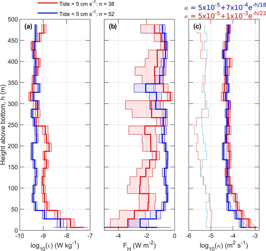
Z. Koenig et al.: Ocean mixing north of Svalbard                                                                                      371

Figure 4. Isopycnally averaged profiles of (a) 2, (b) SA , (c) dissipation rate  and (d) diapycnal diffusivity κ. The profiles are shown
using the average depth of the isopycnals. (e) θ –SA diagram. Profiles are selected relative to the distance from the 800 m isobath: −10 km
(red) inshore, at the shelf break in the Atlantic Water core (blue), and 10 km offshore (green). In the legend, n indicates the number of
batch-averaged profiles used in each average.

intense dissipation of lee waves driven by cross-slope tidal            and κ), the geometric mean (GM) characterizes the distri-
currents (Fer et al., 2020b). Process station P in the Nansen           bution’s central tendency while the arithmetic mean (AM)
Basin far from the continental slope (Fig. 1) is a 24 h pro-            tends to be disproportionately skewed by a small number of
cess study at a surface thermohaline front (Fig. 3g). At this           large values (Scheifele et al., 2020). AM characterizes the in-
specific station, turbulence structure in the mixed layer was           tegrated effect of the distribution and is representative of the
generally consistent with turbulence production through con-            cumulative effect of mixing and average buoyancy transfor-
vection by heat loss to the atmosphere and mechanical forc-             mations produced by mixing (Scheifele et al., 2020).
ing by moderate wind (Koenig et al., 2020).
   In the following sections, we will first examine the mixed
layer evolution from summer to fall and the role of wind                4     Upper layer dynamics
forcing. Then we will investigate the turbulence structure in
the deeper layers, forced by tidal currents. Using the mea-             4.1    Seasonal evolution
surements in the Atlantic Water layer we quantify the verti-
cal heat loss from the Atlantic Water layer. Basic statistics           Solar heating melts the sea ice, which has consequences
(arithmetic and geometric mean and standard deviations) of              for the upper ocean dynamics. Throughout the summer,
mixing parameters for July and September are summarized                 the mixed layer becomes fresher and lighter (34.9 g kg−1
in Table 2. We used both arithmetic and geometric means                 and 27.7 kg m−3 in July, and 34 g kg−1 and 26.95 kg m−3 in
to describe the dissipation rates, diffusivity and turbulent            September; Fig. 5) and also deepens (18 m in July and 23 m
fluxes. For variables with lognormal distribution (such as             in September). This evolution in summer towards a lighter
                                                                        mixed layer is mainly due to the meltwater during the sum-

https://doi.org/10.5194/os-17-365-2021                                                                  Ocean Sci., 17, 365–381, 2021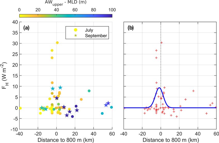
372                                                                                    Z. Koenig et al.: Ocean mixing north of Svalbard

Table 2. Statistics of the turbulence variables measured in July and September. AM: arithmetic mean; GM: geometric mean; σ : standard
deviation; D : vertically integrated dissipation rate; : dissipation rate; κ: diffusivity; FH : vertical turbulent heat flux (positive upward). Four
layers are defined. MLD: ±10 m around the base of the mixed layer; AWcore –MLD: from the Atlantic Water core to the mixed layer depth;
AW layer: in the Atlantic Water layer; and AWcore –bottom: from the Atlantic Water core to the seafloor. The geometric mean is ill-defined
for negative values and hence not provided for the turbulent heat fluxes.

                                                                                   July                  September
                                                                            AM      GM        σ      AM      GM         σ
                           D × 10−4 (W m−2 )         MLD                    1.3     0.3    2.5       1.8     0.3     4.6
                                                      AWcore –MLD            3.1     0.6    7.2       3.8     0.7     8.3
                                                      AW layer               8.9     5.0   12.8       8.7     4.8    12.8
                                                      AWcore –bottom         9.3     6.2     12       9.6     6.4    12.0
                            × 10−9 (W kg−1 )         MLD                  23.7      5.3   56.5      28.4     5.5    67.6
                                                      AWcore –MLD          18.8      4.4   50.1      22.6     4.8    55.5
                                                      AW layer              4.1      1.7   10.3         4     1.7    10.3
                                                      AWcore –bottom        3.9      1.5   10.3       3.9     1.6    10.3
                           κ × 10−5 (m2 s−1 )         MLD                   6.9      3.9    6.9        38       4     221
                                                      AWcore –MLD           5.4      2.6    7.7      16.6     3.0    64.8
                                                      AW layer             10.9      7.6   13.3       9.8     6.5    13.2
                                                      AWcore –bottom       11.1      7.9   13.3      10.5     7.4    13.1
                           FH (W m−2 )                MLD                   2.5        –   18.4      3.6        –    17.6
                                                      AWcore –MLD           4.4        –   11.4      3.0        –     8.9
                                                      AW layer             −1.4        –    1.6     −1.4        –     1.7
                                                      AWcore –bottom       −1.5        –    1.6     −1.4        –     1.6

mer. In both summer and fall, dissipation rates, buoyancy
fluxes and turbulent heat fluxes increased at the base and just
below the mixed layer compared to the rest of the water col-
umn (Fig. 5 and Table 2).
   The depth-integrated dissipation rate at the base of the
mixed layer Dml is on average about (1–2) × 10−4 W m−2
during both cruises, with a geometric mean of about 3 ×
10−5 W m−2 (Table 2). Turbulent buoyancy fluxes in the
mixed layer are directed downward, and turbulent salt fluxes
upward, in both July and September. Salt and buoyancy
fluxes are larger in September than in July at the base of the
mixed layer: the salt flux is 4.2 × 10⁻⁴ kg s−1 m−2 in July
and 1.1 × 10⁻³ kg s−1 m−2 in September, and the buoyancy
flux is −2.4×10⁻⁹ W kg−1 in July and −5.3×10⁻⁹ W kg−1
in September, as the meltwater content in the upper layer is
larger in September than in July.
   Turbulent heat fluxes across the base of the mixed layer
are positive (upward) in both July and September, but larger
in September than in July (3.6 and 2.5 W m−2 respectively).
                                                                             Figure 5. θ –SA diagrams where the color-coded bins are dissipation
The turbulent heat fluxes measured during both cruises are                   rate (a, d), turbulent heat flux (b, e) and magnitude of buoyancy
comparable to what is observed under the sea ice in the                      flux (c, f; the buoyancy fluxes are all oriented downward). Contours
absence of forcing events during the N-ICE2015 experi-                       are σ0 , referenced to surface pressure. Panels (a), (b) and (c) are for
ment (Meyer et al., 2017; Peterson et al., 2017) (about                      summer (July cruise) and (d), (e) and (f) for fall (September cruise).
2 W m−2 ), but about 1/40 to 1/30 times the heat fluxes (up                  The green star is the mean temperature and salinity property of the
to 100 W m−2 ) observed during storm events above the con-                   mixed layer in July and the purple circle is the corresponding value
tinental slope. Variations in the density field are dominated                in September.

Ocean Sci., 17, 365–381, 2021                                                                        https://doi.org/10.5194/os-17-365-2021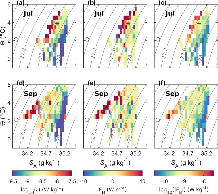
Z. Koenig et al.: Ocean mixing north of Svalbard                                                                                      373

by the variations in salinity; thus buoyancy and salt fluxes
vary concomitantly.

4.2    Wind forcing

Wind stress at the ocean surface is one of the main drivers for
the upper layer turbulence and can increase the ocean-to-ice
heat fluxes (Meyer et al., 2017; Dosser and Rainville, 2016).
A fraction of the wind energy flux from the atmosphere to
the ocean then fuels turbulence in the upper ocean and is dis-
sipated in the mixed layer. Using the observed dissipation in
the mixed layer and the wind energy input (Fig. 6), we ob-
                              (1.4±0.2)
tain a line fit: Dml = 0.002E10         , where Dml is the depth-
integrated dissipation rate in the mixed layer. Observations in
September are limited as only a few stations were performed
with the VMP.                                                       Figure 6. Depth-integrated dissipation rate in the mixed layer, Dml ,
   For relatively low values of E10 (less than 6.3 ×                as a function of the wind energy input to the mixed layer, E10 .
                                                                    Stars and circles are data from the September and July cruises, re-
10−1 W m−2 ), the relation is almost linear, suggesting that
                                                                    spectively. The red circle is the data point from the RS2 process
about 1 ‰ of wind energy input is dissipated in the mixed           station where nonlinear internal waves were observed (Fer et al.,
layer. For larger E10 , additional processes such as breaking       2020b). The green star is the data point at the process station at a
gravity waves can contribute. During the cruise in Septem-          front in September where convection was also important (Koenig
ber, the surface waves were characterized by 0.5–1.5 m sig-         et al., 2020). The black line is the regression line, with the equation
nificant wave height (Sect. 3.1, Løken et al., 2019). Because       indicated. The uncertainty is the 95 % confidence interval.
the dissipation measurements are contaminated by the ship’s
wake in the upper 10 m, we cannot resolve the role of wave-
boundary layer dynamics on the vertical structure of dissipa-       cent. The barotropic-to-baroclinic energy conversion from
tion. Since the wave forcing in September was weak, we do           the tidal activity results in trapped linear waves that can only
not expect a substantial contribution to the observed nonlin-       propagate along topography guidelines, or a nonlinear re-
ear dependence of mixed-layer dissipation on wind energy            sponse with properties similar to lee waves (Vlasenko et al.,
input. However, the relatively large values of Dml in July          2003; Musgrave et al., 2016). A fraction of the energy in
when E10 was large (circles in Fig. 6) might be associated          trapped waves or nonlinear waves will dissipate locally, lead-
with surface waves.                                                 ing to substantial vertical mixing (Padman and Dillon, 1991).
   The front process station P (green star) is more energetic       In our observations, the dissipation rate below the mixed
than what is expected from only wind forcing as convection          layer is typically low (Table 2), but energetic turbulence ob-
is active on the warm side of the front (Koenig et al., 2020).      served at some locations (Fig. 3) can be related to tidal forc-
Dissipation in the mixed layer at RS2 (red circle) is only          ing.
computed using the first casts as there is no data in the shal-        We select the profiles of turbulent heat fluxes and dissipa-
low mixed layer during the intense dissipation event driven         tion rates in categories of tidal current speed predicted from
by cross-slope tidal currents (Fig. 3f). The presence of sea        Arc5km2018 at the time of the measurement. Tidal current
ice in the region can also explain the nonlinearity of the re-      speed is defined as high (> 5 cm s−1 ) or low (< 5 cm s−1 )
lation between the wind energy and the energy dissipation in        (Fig. 7). The profiles in the corresponding categories are av-
the mixed layer. Although the profiles were collected in ice-       eraged with respect to height above bottom defined as the
free conditions, some stations were close to the sea ice edge       difference between the depth of the measurement and the
spotted from the ship.                                              seafloor depth. We obtained the average profiles as the max-
                                                                    imum likelihood estimator from a lognormal distribution us-
                                                                    ing the data points in 20 m vertical bins. The mixed layer was
5     Tidal mixing                                                  excluded in all the profiles to minimize the contribution from
                                                                    dissipation driven by surface processes.
Previous observations show that north of Svalbard is a re-             From the seafloor to about 250 m height above bottom, the
gion of substantial tidal mixing (Rippeth et al., 2015; Fer         dissipation rate was larger ( > 10−8 W kg−1 ) in conditions
et al., 2015). The location is northward of the critical lati-      with strong tidal currents compared to weaker tidal currents
tude of the main diurnal and semidiurnal tidal components           ( < 5×10⁻⁹ W kg−1 ). In both cases, the dissipation rate de-
(K1 and M2 ). The critical latitude, also called the turning lat-   creases quickly with height from the seafloor, down to dis-
itude, is where the tidal frequency matches the local inertial      sipation rates of ∼ 5 × 10⁻¹⁰ W kg−1 above 250 m from the
frequency. The linear response at high latitudes is evanes-         bottom. The increase in dissipation rates for strong tidal forc-

https://doi.org/10.5194/os-17-365-2021                                                                Ocean Sci., 17, 365–381, 2021
374 Z. Koenig et al.: Ocean mixing north of Svalbard
Figure 7. Average profiles of (a) dissipation rate , (b) turbulent heat flux FH and (c) diapycnal diffusivity κ for small (blue) and large (red)
tidal current amplitudes estimated from Arc5km2018 at the time and location of each station. Average profiles are obtained as the maximum
likelihood estimator from a lognormal distribution using the data points in 20 m vertical bins. The vertical axis is height above bottom,
relative to the seafloor depth from the echo sounder. n indicates the number of batch-averaged profiles for each tidal forcing category. Thin
lines in (c) are the corresponding profiles for diffusivity at the lowest detection level (obtained by imposing a noise level for the dissipation
rate of 1×10⁻¹⁰ W kg−1 ). The dashed lines are the curve fits using an exponential function. Resulting equations with the best-fit coefficients
are shown above the panel. The shading is the 95 % confidence envelope of the maximum likelihood.
ing is associated with an absolute increase in the downward high and low tidal current speeds are shown above Fig. 7c.
turbulent heat flux close to seafloor: −2.2 W m−2 when tidal With large tidal amplitudes, κbot approximately doubles and
currents were weak and about −3.2 W m−2 when tidal cur- the decay scale increases from 18 to 22 m (95 % confidence
rents were strong. interval of 2 m).
Similar to the dissipation rate, the diapycnal diffusivity We investigate the role of two distinct contributions from
decreases with increasing height above bottom (Fig. 7c). tidal currents to the turbulent mixing. While tidally driven
Based on the observations from north of Svalbard, we can processes may lead to interior mixing away from the seabed
deduce an empirical relation that would allow an estimate (Fer et al., 2020b), bottom stress from barotropic tidal cur-
of the diffusivity in conditions of strong (> 5 cm s−1 ) or rents must be balanced by dissipation in bottom boundary
weak (< 5 cm s−1 ) tidal currents. Following St. Laurent et al. layers. The tidal work can be representative of the barotropic-
(2002), we use a functional form for the diffusivity expressed to-baroclinic conversion and can be related to the dissipation
as follows: of propagating or trapped internal wave energy, which can
likely extend far into the water column. In the bottom bound-
κ = κbg + κbot × e−h/zdecay , (5) ary layer, the bottom stress from the barotropic tide also plays
a role. The relative contributions to mixing through the tidal
where κbg is a background diffusivity, κbot is the diffusivity work and the tidally driven bottom drag are unknown.
value at the seafloor, h is the height above bottom and zdecay We analyze the vertically integrated dissipation rate in the
is the vertical decay scale of the diffusivity. We use κbg = bottom 250 m of the water column D250 (and below the sur-
5 × 10⁻⁵ m2 s−1 , based on observations. Fitted equations for
Ocean Sci., 17, 365–381, 2021 https://doi.org/10.5194/os-17-365-2021Z. Koenig et al.: Ocean mixing north of Svalbard 375
face mixed layer) separately with respect to tidal work and
the tidally driven bottom drag (Fig. 8). The total rate of
work by barotropic tidal currents interacting with topography
was computed as the product of the Baines force (Baines,
1982) and the barotropically induced vertical velocity fol-
lowing Nash et al. (2006), for the main diurnal and semid-
iurnal constituents. D250 does not correlate well with the
tidal work, Wtidal , at the time of observations (not shown).
A least-squares power-law fit results in an uncertainty of
the power which is more than 50 % of its estimated value:
0.16±0.09
D250 = 7 × 10⁻³ Wtidal .
The tidally driven bottom drag is examined next, expressed
as in Jayne and St. Laurent (2001): Figure 8. Depth-integrated dissipation rate in the bottom 250 m
3 (D250 ) regressed against (a) the instantaneous tidally driven bottom
Wbotdrag = ρ0 Cd |u| , (6)
drag and (b) the typical tidally driven bottom drag (using urms ). See
where Cd is the bottom drag coefficient, ρ0 is the seawater text for details. Linear fits on the logarithmic parameter space (i.e.,
density and u is the tidal current vector. Note that this equa- power-law fits) denoted by the black lines, and the corresponding
tion is analogous to the drag relation for the wind energy flux equations are indicated with the 95 % confidence levels. Red dots
are the data points from the RS2 station. Process stations are batch-
E10 (in Sect. 4.2). In calculations two different tidal currents
averaged (in sets of 4–5 consecutive profiles) in (a) and averaged
are used: the instantaneous tidal speed ut at the time and loca-
over the station duration in (b).
tion of each station and a statistical estimate of the represen-
tative cross-isobath tidal current, urms , at the location of each
station (Fig. 8). Both are obtained from the Arc5km2018 useful parameterization to infer vertically integrated dissipa-
model. We calculated urms from the predicted local cross- tion rates. An estimate along the margin of the Eurasian basin
isobath component of the tidal currents over an arbitrary 30 d will be given in the discussion using the relation in Fig. 8b.
window using all constituents; this choice offers a parameter
easily available for parameterization purposes, independent
of observations. 6 Mixing in the Atlantic Water layer
In analyzing the vertically integrated dissipation rates with
respect to local forcing at the time of observations (Fig. 8a), As the heat content in the Atlantic Water in the Arctic Ocean
we averaged the process stations in batches as explained in has the potential to melt the sea ice cover completely, it is
Sect. 3; this allows for including some time variability in the important to quantify the turbulent dissipation rates and heat
observations. For the analysis of typical tidal forcing, we av- fluxes out of the Atlantic Water in the new conditions of a
eraged each process station as one data point because each warming Arctic. The depth-integrated dissipation rate from
location is associated with a time-independent urms (Fig. 8b). the base of the mixed layer to the Atlantic Water core is about
The local bottom drag at the time of observations correlates 8.8 × 10⁻⁴ W m−2 , and the average dissipation rate is about
well with D250 and follows the power-law fit with a con- 2 × 10⁻⁸ W kg−1 , almost as large as what is observed in the
siderable scatter (uncertainty of the power is less than 25 % mixed layer (Table 2). We estimated the vertical turbulent
its estimated value; Fig. 8a). This nonlinear relationship be- heat flux between the upper limit of the Atlantic Water layer
tween D250 (dissipation in the bottom 250 m) and Wbotdrag and the mixed layer depth (Fig. 9a), in both summer and fall.
shows parallels with the nonlinear relationship between Dml The maximum positive heat flux (upward toward the surface)
(dissipation in the surface mixed layer) and E10 . If we force is observed near the 800 m isobath, reaching up to 30 W m−2
a linear relation in panel (a), we find a drag coefficient of in July and 10 W m−2 in September. This isobath is repre-
Cd = 8.2×10⁻⁴ . This value is comparable to but smaller than sentative of the average location of the core of Atlantic Water
the typical range of bottom drag values of (1–3) × 10−3 and (Kolås et al., 2020). Outside the Atlantic Water boundary cur-
the bottom drag deduced from in situ observations in Bering rent, about 20 km inshore and offshore from the 800 m iso-
Strait of 2.3 × 10⁻³ (Couto et al., 2020). The red data points bath, vertical turbulent heat fluxes are negligible, with a max-
in Fig. 8 are from the station RS2, where energetic turbulence imum of 5 W m−2 . In July, the Atlantic Water core tends to be
was observed from dissipation of nonlinear internal waves closer to the base of the mixed layer compared to September
(Fer et al., 2020b). It partly explains why larger dissipation (Fig. 9a), implying that the heat contained in the Atlantic Wa-
rates are observed here than what could be expected from ter is more likely to reach the surface in July than in Septem-
the tidally driven bottom drag alone. The analysis is repeated ber. Meltwater in September enhances the stratification near
using the bottom drag parameters calculated using the typi- the surface and isolates the Atlantic Water layer from the
cal cross-isobath tidal forcing urms (Fig. 8b). The scatter is mixed layer. At some stations, vertical turbulent heat fluxes
reduced, and in particular the bottom-drag relation offers a are negative (0 to −5 W m−2 ), directed downward from the
https://doi.org/10.5194/os-17-365-2021 Ocean Sci., 17, 365–381, 2021376 Z. Koenig et al.: Ocean mixing north of Svalbard
7 Discussion
7.1 Estimates of the tidally driven dissipation rate in
the Eurasian Basin
Turbulent mixing in the Arctic is not well-documented, and
measurements close to the bottom are scarce. The bottom
drag estimated from the Arc5km2018 predictions in the Arc-
tic Ocean, using a constant drag coefficient, is larger on the
shelf and on the ridges than in the deep basin (not shown),
as a result of sensitivity to the strength of the barotropic tidal
current. These areas coincide with regions of enhanced tidal
activity in the Arctic (Padman and Erofeeva, 2004). Using
this tidally driven bottom drag and the relation inferred from
Figure 9. (a) Lateral distribution of the mean vertical turbulent heat the data collected north of Svalbard (Sect. 5 and equation in
flux from the AW upper boundary to the base of the mixed layer. Fig. 8b), we estimate the depth-integrated dissipation rate.
The horizontal axis is the horizontal distance to the 800 m isobath. The highest bottom depth-integrated dissipation rates in the
The color code is the vertical distance between the upper boundary Arctic are found on the shelves and are consistent with the
of the Atlantic Water layer and the mixed layer depth. Markers iden- pan-Arctic observations compiled and presented in Rippeth
tify the stations collected in July (circles) and September (stars). et al. (2015), reaching 10−3 W m−2 (not shown).
(b) A Gaussian fit (blue line) to the vertical turbulent heat flux from Because the parameterization is obtained using a limited
the Atlantic Water to the mixed layer depth (red crosses).
dataset from a localized region north of Svalbard, instead of
presenting Arctic-wide maps we concentrate on the Eurasian
surface toward the Atlantic Water layer. The negative fluxes Basin from north of Svalbard into the East Siberian Sea. The
are mainly found near the core of the Atlantic Water inflow. cross-isobath tidal currents along this transect, particularly
These negative heat fluxes are observed when warm water in the Laptev Sea, are strong (see Fig. 1 of Fer et al., 2020b).
reaches the surface, and the temperature increases from the Figure 10 shows the time-averaged cross-isobath tidal cur-
top of the Atlantic Water layer up to the surface. This situa- rent amplitude, and the depth-integrated dissipation rate in
tion is typical of summer conditions north of Svalbard where the bottom 250 m estimated using the equation in Fig. 8b,
the Atlantic Water extends close to the surface and the cold along the continental slope of the Eurasian basin. The largest
halocline is absent (Polyakov et al., 2017). tidal speeds are observed north of Svalbard and in the east-
The lateral (cross-isobath) distribution of the diapycnal ern part of the Laptev Sea where the slope connects to the
heat fluxes is similar in July and September (Fig. 9a). We Lomonosov Ridge, reaching more than 0.1 m s−1 (Fig. 10a).
therefore used all data points to fit a Gaussian curve (Fig. 9b), The largest average bottom dissipation rates across the con-
with an aim to estimate the integrated heat loss from the At- tinental slope are observed at 35◦ E, just east of Svalbard
lantic Water layer. Between −20 and +20 km, the heat loss and at the Lomonosov Ridge, reaching 3.2 × 10⁻⁴ W m−2 .
due to vertical turbulent heat fluxes is about 1.2×10⁵ W m−1 . We present two estimates for the dissipation: the vertically
Using independent hydrographic observations but covering integrated dissipation rate in the bottom 250 m, D250 , aver-
the same observational time period, Kolås et al. (2020) found aged laterally between the 400 and 1200 m isobaths (blue
that the average along-path change of heat content from sec- line and left axis; Fig. 10b), and D250 integrated meridion-
tion B to E was about 9.1 × 10⁷ W m−1 , and about 9.6 × ally between the 400 and 1200 m isobaths (red line and right
106 W m−1 from section C to D, corresponding to an aver- axis; Fig. 10b). This volume-integrated dissipation rate, per
age heat loss of about 500 W m−2 north of Svalbard. Heat unit meter along the shelf break, shows variations similar to
loss from the Atlantic Water layer by vertical turbulent heat the averaged D250 , except at 70◦ E. This is the location of
fluxes to the upper ocean then accounts for only about 1 % the Santa Anna Trough, where the Atlantic Water from the
of the total Atlantic Water heat loss north of Svalbard. This Barents Sea flows into the Arctic Ocean and where the dis-
estimate can be biased low since during the period of mea- tance between the 400 and 1200 m isobaths triples compared
surements wind forcing was weak to moderate with low vari- to the rest of the Eurasian continental slope. Rippeth et al.
ability. Processes that contribute to the turbulent heat loss of (2015) argued, based on microstructure measurements and
the Atlantic Water layer are discussed in Sect. 7. tidal velocities from the TPXO8 inverse solution, that the en-
ergy supporting much of the enhanced dissipation along the
continental slopes in the Eurasian Basin, and more specifi-
cally north of Svalbard and around the Lomonosov Ridge, is
of tidal origin. The mean-integrated dissipation over the At-
lantic layer observed in Rippeth et al. (2015) is of a similar
Ocean Sci., 17, 365–381, 2021 https://doi.org/10.5194/os-17-365-2021Z. Koenig et al.: Ocean mixing north of Svalbard 377
order of magnitude to the depth-integrated dissipation in the by these nonlinear waves is also noticeable in Fig. 8a and c
bottom 250 m deduced from the tidally driven bottom drag as (the red dots). At this location, the inverse Froude number for
observed in our study. However, the bottom depth-integrated the diurnal frequency exceeds 3, supporting the interpretation
dissipation rate extrapolated from a local relation valid north that such conditions can favor the development of nonlinear
of Svalbard to the Arctic Ocean must be considered with cau- processes.
tion.
As the Eurasian Arctic is poleward of the critical latitude
7.2 Atlantic Water heat loss
for most of the main tidal constituents, the response to tidal
flow over sloping topography can be nonlinear when the to-
pographic obstruction of the stratified flow is large. Legg The Atlantic Water loses heat as it propagates cyclonically
and Klymak (2008) proposed that an inverse Froude num- along the continental slope in the Arctic Ocean. Around
ber, Fr−1
ω , based on a vertical excursion distance of the tidal the Yermak Plateau, the along-path cooling and freshening
current over bottom slope, can be used to estimate the possi- are estimated to be 0.2 ◦ C per 100 km and 0.01 g kg−1 per
bility of occurrence of highly nonlinear jump-like lee waves, 100 km, corresponding to a surface heat flux between 400
such as those observed at station RS2 (Fer et al., 2020b) or and 500 W m−2 (Boyd and D’Asaro, 1994; Cokelet et al.,
modeled over the Spitsbergen Bank (Rippeth et al., 2017), 2008; Kolås and Fer, 2018). We found that the upward heat
a shallow bank south of Svalbard and poleward of the M2 loss from turbulent heat fluxes from the Atlantic Water layer
critical latitude. The inverse Froude number is expressed as up to the mixed layer reached on average 8 W m−2 . This fig-
follows: ure is 1 order of magnitude larger than vertical heat flux from
|∇H| N the Atlantic Water to the surface in the Laptev Sea (on the
Fr−1
ω = , (7) order of 0.1–1 W m−2 , Polyakov et al., 2019). North of Sval-
ω bard and in the Laptev Sea, heat loss due to turbulent vertical
where |∇H| is the bottom slope and ω is the tidal frequency. mixing represents less than 10 % of the total heat loss of the
In our calculations we used the Brunt–Väisälä frequency N Atlantic Water (Kolås et al., 2020; Polyakov et al., 2019).
near the bottom, extracted from the MIMOC climatology in Ivanov and Timokhov (2019) estimated that from the Yer-
August (the result is not sensitive to this choice as the near- mak Plateau to the Lomonosov Ridge, 41 % of the Atlantic
bottom stratification does not have a strong seasonal cycle). Water heat is lost to atmosphere, 31 % to deep ocean and
When Fr−1 ω > 3, the vertical excursion distance induced by 20 % is lost laterally. Heat loss resulting from vertical heat
tidal currents is sufficiently large that hydraulic jumps could fluxes contributes to the heat loss to the atmosphere and to the
occur and nonlinear waves can develop (Legg and Klymak, deep ocean, but not to the lateral heat loss. Several processes
2008). The calculations along the Eurasian shelf break are can lead to lateral heat loss north of Svalbard, including eddy
presented in Fig. 10c for the semidiurnal and the diurnal tidal spreading from the slope into the basin (Crews et al., 2018;
forcing. Along the Eurasian slope, we expect nonlinear inter- Våge et al., 2016). Using eddy-resolving regional model re-
nal waves to develop for the diurnal tidal forcing in the east- sults, Crews et al. (2018) found that eddies export 1.0 TW
ern part of the Kara and Laptev seas, where Fr−1 ω is much out of the boundary current, delivering heat into the inte-
larger than 3, the threshold value for the development of non- rior Arctic Ocean at an average rate of ∼ 15 W m−2 . West
linear processes. Values slightly above this threshold are also of Svalbard, Kolås and Fer (2018) found that the measured
observed north of Svalbard. In the region north of Svalbard turbulent heat flux in the WSC was too small to account for
and in the eastern part of the Laptev Sea, the large depth- the cooling rate of the Atlantic Water layer but reported a
integrated dissipation rate observed in Fig. 10b can be driven substantial contribution from energetic convective mixing of
by nonlinear waves implied by the peaks of Fr−1 ω (Fig. 10c). an unstable bottom boundary layer on the slope. Convection
These two areas warrant further studies. In the eastern part of was driven by the Ekman advection of buoyant water across
the Kara Sea, however, the depth-integrated dissipation rates the slope and complements the turbulent mixing in the cool-
are relatively low despite the large inverse Froude number ing process. The estimated lateral buoyancy flux was about
values that suggest nonlinear processes could develop there. 10−8 W kg−1 (Kolås and Fer, 2018), sufficient to maintain
North of Svalbard, observations of nonlinear internal a large fraction of the observed dissipation rates, and corre-
waves were documented in Fer et al. (2020b) during the July sponds to a heat flux of approximately 40 W m−2 . We can
cruise at RS2. They showed abrupt isopycnal vertical dis- expect similar processes to extract heat and salt from the At-
placements of 10–50 m and an intense dissipation associated lantic Water core north of Svalbard. Such processes can ex-
with cross-isobath diurnal tidal currents of ∼ 0.15 m s−1 . The plain why turbulent heat fluxes are only responsible for 10 %
dissipation of these nonlinear internal waves creates an in- of the Atlantic heat loss north of Svalbard. Furthermore, large
crease in dissipation in the whole water column by a factor heat loss during extreme events should not be ignored. For
of 100 and turbulent heat fluxes are about 15 W m−2 com- example, Meyer et al. (2017) found that the average heat flux
pared with the background turbulent heat flux of 1 W m−2 of about 7 W m−2 across the 0 ◦ C isotherm increased during
(Fer et al., 2020b). The increase in the dissipation rate driven storms, exceeding 30 W m−2 . During our survey, without ex-
https://doi.org/10.5194/os-17-365-2021 Ocean Sci., 17, 365–381, 2021You can also read