Development of the Real-time On-road Emission (ROE v1.0) model for street-scale air quality modeling based on dynamic traffic big data
←
→
Page content transcription
If your browser does not render page correctly, please read the page content below
Geosci. Model Dev., 13, 23–40, 2020
https://doi.org/10.5194/gmd-13-23-2020
© Author(s) 2020. This work is distributed under
the Creative Commons Attribution 4.0 License.

Development of the Real-time On-road Emission (ROE v1.0) model
for street-scale air quality modeling based on dynamic
traffic big data
Luolin Wu1 , Ming Chang2 , Xuemei Wang2 , Jian Hang1 , Jinpu Zhang3 , Liqing Wu1 , and Min Shao2
1 Schoolof Atmospheric Sciences, Sun Yat-sen University, Guangzhou 510275, P. R. China
2 Institute
         for Environmental and Climate Research, Jinan University, Guangzhou 510632, P. R. China
3 Guangzhou Environmental Monitoring Center, Guangzhou 510030, P. R. China

Correspondence: Xuemei Wang (eciwxm@jnu.edu.cn)

Received: 25 March 2019 – Discussion started: 10 April 2019
Revised: 3 July 2019 – Accepted: 13 August 2019 – Published: 3 January 2020

Abstract. Rapid urbanization in China has led to heavy traf-      tochemistry in the urban areas by using the on-road emission
fic flows in street networks within cities, especially in east-   results from the ROE model. The modeling results indicate
ern China, the economically developed region. This has in-        that the daytime NOx concentrations on national holidays are
creased the risk of exposure to vehicle-related pollutants.       26.5 % and 9.1 % lower than those on normal weekdays and
To evaluate the impact of vehicle emissions and provide an        normal weekends, respectively. Conversely, the national hol-
on-road emission inventory with higher spatiotemporal res-        iday O3 concentrations exceed normal weekday and normal
olution for street-network air quality models, in this study,     weekend amounts by 13.9 % and 10.6 %, respectively, owing
we developed the Real-time On-road Emission (ROE v1.0)            to changes in the ratio of emission of volatile organic com-
model to calculate street-scale on-road hot emissions by us-      pounds (VOCs) and NOx . Thus, not only the on-road emis-
ing real-time big data for traffic provided by the Gaode          sions but also other emissions should be controlled in order
Map navigation application. This Python-based model ob-           to improve the air quality in Guangzhou. More significantly,
tains street-scale traffic data from the map application pro-     the newly developed ROE model may provide promising and
gramming interface (API), which are open-access and up-           effective methodologies for analyzing real-time street-level
dated every minute for each road segment. The results of ap-      traffic emissions and high-resolution air quality assessment
plication of the model to Guangzhou, one of the three major       for more typical cities or urban districts.
cities in China, showed on-road vehicle emissions of carbon
monoxide (CO), nitrogen oxide (NOx ), hydrocarbons (HCs),
PM2.5 , and PM10 to be 35.22 × 10⁴ , 12.05 × 10⁴ , 4.10 × 10⁴ ,
0.49 × 10⁴ , and 0.55 × 10⁴ Mg yr−1 , respectively. The spa-      1   Introduction
tial distribution reveals that the emission hotspots are lo-
cated in some highway-intensive areas and suburban town           Rapid economic development and urbanization have led to an
centers. Emission contribution shows that the dominant con-       exponential growth in the number of vehicles in China in re-
tributors are light-duty vehicles (LDVs) and heavy-duty vehi-     cent years (National Bureau of Statistics of China, 2017). As
cles (HDVs) in urban areas and LDVs and heavy-duty trucks         one of the three major urban clusters, the Pearl River Delta
(HDTs) in suburban areas, indicating that the traffic con-        (PRD) region, or its main city Guangzhou, has experienced a
trol policies regarding trucks in urban areas are effective.      significant increase in the number of vehicles. This increase
In this study, the Model of Urban Network of Intersecting         has become the dominant contributor to carbon monoxide
Canyons and Highways (MUNICH) was applied to investi-             (CO), nitrogen oxide (NOx ), and hydrocarbon (HC) emis-
gate the impact of traffic volume change on street-scale pho-     sions (He et al., 2002; Zheng et al., 2009a), which in turn
                                                                  are causing more frequent and more severe public health

Published by Copernicus Publications on behalf of the European Geosciences Union.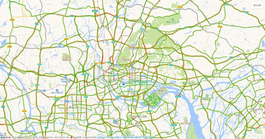
24                                         L. Wu et al.: Development of the Real-time On-road Emission (ROE v1.0) model

problems in Chinese megacities (An et al., 2013). Previous          Therefore, spatial distribution is directly obtained from the
studies have shown that on-road vehicle emissions can con-          input data and spatial and temporal allocations are not re-
tribute approximately 22 %–52 % of total CO, 37 %–47 % of           quired. Among the input data, the traffic data are crucial for
total NOx , and 24 %–41 % of total HC emissions detected in         establishing the inventories and determining their accuracy.
cities (Zhang et al., 2009; Zheng et al., 2009a, 2014; Li et al.,   Some previous studies have used traffic simulation models to
2017).                                                              obtain traffic speed or volume data of road networks (Palla-
   Reliable on-road emission inventories can be used as input       vidino et al., 2014; Zhang et al., 2016; Chen et al., 2017;
data for the numerical air quality models which are applied         Ibarra-Espinosa et al., 2018). Based on the traffic model, the
to estimate the impact of on-road emissions on the urban air        method could provide traffic data for each road from low-
quality (Wang and Xie, 2009; He et al., 2016). For this pur-        resolution average data. However, the results from such traf-
pose, a realistic on-road vehicle emission inventory should be      fic models may not reflect reality, thereby reducing the ac-
developed for this pollution source. The two main method-           curacy of the inventories. Many other studies have used real-
ologies used in recent years to establish such inventories are      istic traffic data, namely road-side or on-board observational
top-down and bottom-up techniques.                                  data obtained at certain road segments, to establish inven-
   Top-down methods, such as that used in the MOBILE                tories and improve their accuracy (Huo et al., 2009; Wang
model devised by the US Environmental Protection Agency             et al., 2008, 2010; Wang and Xie, 2009; Yao et al., 2013).
(EPA, 2003) and other similar macroscale models, first re-          Although the observed traffic data are helpful for inventory
quire information on vehicle population, vehicle kilometers         establishment, their limitation is obvious in that large-scale
traveled (VKT), and mean vehicle speed for an entire city           observation for a whole city requires extensive human labor
to calculate the total amount of vehicular emissions. Then,         and financial and material resources, which are expensive
the emissions are allocated to each grid cell utilizing param-      and time consuming. Moreover, such observations may not
eters such as road density and road hierarchy (Saide et al.,        provide real-time traffic data, thereby reducing the temporal
2009; Jing et al., 2016; Liu et al., 2018). Many studies have       resolution of the inventories.
adopted this method to develop city- or national-level vehi-           Recent developments in image identification technology
cle emission inventories in China (Hao et al., 2000; Cai and        and other observation detectors are facilitating easy collec-
Xie, 2007; Guo et al., 2007; Saide et al., 2009; Zheng et al.,      tion of real-time traffic data from road networks. The exten-
2009a; Sun et al., 2016). However, the top-down inventories         sive implementation of closed-circuit televisions and other
offer low-level spatial and temporal resolutions because of         detection subsystems in cities helps intelligent transport sys-
the allocation method and input data used. Typically, the spa-      tems (ITSs) in China (Wu et al., 2009), making it possible to
tial allocation of a top-down inventory is based on the road        attain real-time traffic data at the city scale. Using the traffic
network. The greater the road density and length, the higher        data provided by ITSs, many previous studies have success-
the amount of emissions in the same grid. This allocation           fully developed inventories for different areas in China (Jing
method simplifies the road emissions by assuming that ev-           et al., 2016; Liu et al., 2018; Zhang et al., 2018). Such stud-
ery road of a specific road type (e.g., highway, arterial road,     ies provided us with a new direction for the establishment
or local road) experiences the same traffic volume irrespec-        of bottom-up inventories. The real-time traffic data from the
tive of its location. In addition, emission factors are consid-     road network could be the most precise input data for on-
ered to remain unchanged despite the traffic speed over the         road emission inventories and could significantly improve
entire city, thereby leading to inaccurate results for the in-      the spatial and temporal resolutions of the inventories. How-
ventory. Moreover, some megacities (e.g., Guangzhou) have           ever, there are still some difficulties in using the ITS data. In
traffic control policies in place in certain urban areas, which     some cities, construction of the ITS is not complete yet or has
implies that the emissions should differ across areas. Besides,     not even been carried out. Moreover, the inconsistency of the
the VKT data are usually provided on the yearly scale, which        data standards leads to an inefficient way of data utilization
limits the temporal resolution of the inventory. For numerical      (Zhang, 2010). Furthermore, the low degree of data sharing
modeling, the accuracy of the emission inventory may have           may be the biggest barrier to using traffic data obtained from
a great impact on the simulation results because of the strong      the ITSs (Huang et al., 2017).
dependence of numerical models on it (Jing et al., 2016).              With the help of a high-resolution emission inventory, nu-
This scale of the emission inventory may not reflect the real       merical models can assess the impact of on-road vehicle
emission conditions for the on-road vehicles within the city,       emissions on the air quality (Huo et al., 2009). The air flow
and thus evaluations of traffic-related impacts on air pollu-       and air quality modeling in cities are commonly categorized
tion in complex situations such as street-level traffic flow are    into four groups by length scales, i.e., street scale (∼ 100 m),
likely to be inaccurate (Huo et al., 2009).                         neighborhood scale (∼ 1 km), city scale (∼ 10 km), and re-
   Consequently, several studies have established higher-           gional scale (∼ 100 km) (Britter and Hanna, 2003). A pre-
resolution inventories using the bottom-up approach. The            vious comprehensive literature review on this topic (Zhang
main difference from the top-down method is that bottom-            et al., 2012) reports that regional-scale chemical transport
up inventories are based on information from road segments.         models (CTMs) have been widely applied to investigate the

Geosci. Model Dev., 13, 23–40, 2020                                                      www.geosci-model-dev.net/13/23/2020/
L. Wu et al.: Development of the Real-time On-road Emission (ROE v1.0) model                                                    25

chemistry and transport of air pollutants from their emission       ROE model outputs the results, i.e., street-level air quality
sources. Many studies have successfully applied regional-           inventories.
scale CTMs to investigate the impact of on-road vehicles on
the air quality in urban areas in the regional scale (∼ 100 km)     2.2   Model structure
(Che et al., 2011; Saikawa et al., 2011; He et al., 2016; Ke et
al., 2017). In addition, some researchers have studied street-      The ROE model was developed to calculate on-road vehi-
scale and neighborhood-scale pollutant dispersion and urban         cle emissions from real-time traffic data. The structure of
air quality by adopting computational fluid dynamics (CFD)          the model is shown in Fig. 1. The model, which has been
models (Fernando et al., 2010; Kim et al., 2012; Kwak et al.,       implemented in Python 3, can be divided into four mod-
2013; Kwak and Baik, 2014; Park et al., 2015; Zhong et al.,         ules: crawler, preprocessing, emissions calculation, and out-
2016; Hang et al., 2017). City-scale (∼ 10 km) CFD mod-             put modules.
eling, however, usually requires consideration of billions of        1. The most crucial part of the emission inventory involves
grids because a city may include tens of thousands of build-            obtaining the real-world traffic data. The crawler mod-
ings with high-resolution and complex street networks (Di               ule is designed for crawling the real-time traffic data
Sabatino et al., 2008; Ashie and Kono, 2011). Thus, as city-            from the ITS, Internet, or any other data source if the
scale CFD simulations are very expensive and time consum-               code is updated to match the format of the data source.
ing, they are currently rare. Recently, some models have been           Moreover, the study area should be set in the mod-
developed and applied to investigate street-level air quality at        ule and, if needed (in case the coordinates differ), the
the city scale (Davies et al., 2007; Righi et al., 2009; Zhang          coordinate transformation script should be activated.
et al., 2016; Kim et al., 2018) by balancing the requirements           The current version of the ROE model includes the
of high resolution and low computational cost.                          crawler module for the https://www.amap.com (last ac-
   In this direction, the first purpose of this study was to find       cess: 2 September 2019) (also called the Gaode Map)
a new open-access source of real-time and high-quality traf-            application (Fig. 2), a widely adopted map application
fic data that could serve as the input for developing an on-            in China (additional details are provided in Sect. 2.4).
road emission inventory with high spatial and temporal reso-
                                                                     2. The preprocessing module is used for fitting the time
lutions for cities or urban districts. Guangzhou was selected
                                                                        frequency between the data source and the air quality
as the target city for the initial application of this method not
                                                                        modeling system. Subsequently, the traffic volume data
only because of the large number of vehicles in use there but
                                                                        are also calculated from the traffic speed data in this
also because of its well-developed ITS which could obtain
                                                                        module if the traffic volume or vehicle fleet informa-
the traffic information from street networks (Xiong et al.,
                                                                        tion is not available from the data source. Otherwise,
2010). A Python-based on-road emission model called the
                                                                        the number of vehicles in each category can be used di-
Real-time On-road Emission (ROE v1.0) model was devel-
                                                                        rectly for the emissions calculation.
oped in this study to utilize these traffic data and establish a
bottom-up on-road emission inventory. A street-level chem-           3. The emissions calculation module uses traffic informa-
istry transport model was then used to apply the emission               tion from the preprocessing module and information
results and study the impact of traffic volume variations on            about vehicle fleets to calculate emissions for each street
the air quality in the urban districts of Guangzhou.                    segment using the following equation:
                                                                               X
                                                                        Es,t =     EFs,v × Vv,t × L,                            (1)

2     Description of the ROE model                                        where Es,t is the emission of pollutant s at time t
                                                                          (g h−1 ), EFs,v is the emission factor of pollutant s for
2.1    Model overview                                                     vehicle category v (g km−1 ), Vv,t is the traffic volume
                                                                          of the vehicle (i.e., the number of vehicles) category v
The ROE model is intended to establish the street-level emis-             at time t (vehicles per hour), and L is the length of the
sion inventories using the emissions of on-road vehicles in               street segment (km). The total emission in one specific
the street segments of interest using a bottom-up approach.               area is given by the sum of emissions in every street
First, the ROE model collects the real-time traffic informa-              segment within the area.
tion to obtain the traffic volume for each street segment from
                                                                     4. The output module sums up all the information given by
the ITS. Then, according to the vehicle fleet information, the
                                                                        the emissions calculation module and can be modified to
ROE model calculates the number of vehicles for each vehi-
                                                                        provide all the results produced during the calculation
cle category on each street segment (if available, these data
                                                                        of the emissions. In addition, the model includes a tool
could be obtained from the ITS and need not be calculated by
                                                                        that can modify the formats of the emissions, making
model). Thereafter, the ROE model calculates the emissions
                                                                        it possible to provide the on-road emissions to other air
for street segments based on the vehicle fleet information,
                                                                        quality models.
traffic conditions, and environmental conditions. Lastly, the

www.geosci-model-dev.net/13/23/2020/                                                        Geosci. Model Dev., 13, 23–40, 2020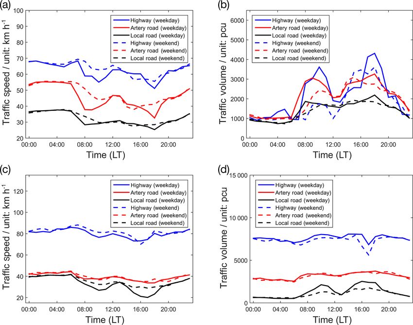
26                                          L. Wu et al.: Development of the Real-time On-road Emission (ROE v1.0) model

Figure 1. The structure of the ROE model.

2.3   Emission factors                                               In addition, the emission factors can be easily updated
                                                                   once the local emission factor data are available.

In this study, nationwide vehicle emission factors mandated
                                                                   2.4   Traffic data from floating car data
by the Ministry of Ecology and Environment (MEP) of the
People’s Republic of China were adopted to calculate the
on-road vehicle emissions (MEP, 2014). They are listed in          In this study, the traffic speed data of each street segment
Tables S1 and S2 in the Supplement. The emission factors of        were obtained from Gaode Map. The Gaode Map traffic data
liquefied petroleum gas (LPG) vehicles were sourced from a         are quite extensive as they cover over 40 cities in China so far
previous study conducted in Guangzhou (Zhang et al., 2013).        (with most of them being major cities). Based on GPS and
According to the MEP guide, vehicles are classified as one         mobile network information, details on vehicle speed and lo-
of the following: a light-duty vehicle (LDV), a middle-duty        cation are collected from the map users’ devices while using
vehicle (MDV), a heavy-duty vehicle (HDV), a light-duty            the map navigation on the road. This aspect saves a consid-
truck (LDT), a middle-duty truck (MDT), a heavy-duty truck         erable amount of human labor and material resources with
(HDT), a motorcycle (MC), a taxi, or a bus. The fuel type          regard to traffic condition observations. These data are up-
is classified as petrol, diesel, or other (such as LPG or nat-     dated in real time and can be used through an open-access
ural gas). The emission standard is classified as Pre-China        application programming interface (API), thus overcoming
I, China I, China II, China III, China IV, or China V. In ad-      the barrier of obtaining data. As the data can be updated in
dition, the evaporation of petrol was considered during the        real time, the emission data can also be refreshed in real time.
calculation of the emissions. HC evaporation was also con-            However, the map application cannot provide the traffic
sidered as per the details provided in the MEP guidebook           volume data directly. Many studies have shown that the traf-
(Table S3).                                                        fic volume can be estimated using the average traffic speed
   The correction factors involving environmental conditions       based on the relationship between the traffic speed and the
(e.g., temperature, relative humidity, and altitude) and traffic   volume (Wang, 2003; Xu et al., 2013; Wang et al., 2013; Yao
conditions obtained from the technical guide were consid-          et al., 2013; Hooper et al., 2014; Jing et al., 2016). Many
ered in the study. They are listed in Tables S4–S10 in the         speed–flow models exist for this purpose and each of them
Supplement. These correction factors were applied to reduce        has certain advantages and disadvantages. In this study, the
the effects of uncertainties associated with the emission fac-     Underwood volume calculation model (Underwood, 1961)
tors.                                                              was used to retrieve the information on traffic volume be-
   To estimate the uncertainties in the emissions factors, the     cause of its history of successful application in China (Jing
results of previous studies (Zheng et al., 2009a; Zhang et al.,    et al., 2016). The model is described by Eq. (2):
2013, 2016; Tang et al., 2016; Wang et al., 2017) were sum-
marized and compared with the emission factors obtained in                       uf
this study. These results appear in Fig. S1 of the Supplement.     V = km u ln      ,                                          (2)
                                                                                 u

Geosci. Model Dev., 13, 23–40, 2020                                                     www.geosci-model-dev.net/13/23/2020/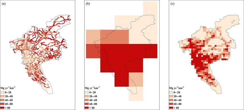
L. Wu et al.: Development of the Real-time On-road Emission (ROE v1.0) model 27
where V is the traffic volume at speed u (vehicles per hour), 3 Description of the street-level air quality model
km is the traffic density (vehicles per kilometer), u is the traf-
fic speed (km h−1 ), and uf is the free speed (km h−1 ). In this To evaluate the impact of on-road emissions on air quality
study, km and uf are given by fitting the model based on at the street level in Guangzhou, an air quality model called
observation data obtained at the roadside and video identi- the Model of Urban Network of Intersecting Canyons and
fication data gained from different road types (Zheng et al., Highways (MUNICH) was employed in this study with the
2009a; Jing et al., 2016; Liu et al., 2018). on-road emission results from the ROE model. MUNICH is
To calculate the traffic volume on national highways, an- a street-network CTM that includes street-canyon and street-
other speed–flow model, which was previously applied in an intersection components in the model (Kim et al., 2018).
observation-based study undertaken in China (Wang, 2003), In this study, the Weather Research and Forecasting
was used. This model is described as follows. (WRF) model (version 3.7.1) (Skamarock et al., 2008)
When the speed limit is 120 km h−1 , was used to provide the meteorological data (wind profile,
boundary-layer height, and friction velocity) for the model-
V = −0.611u2 + 73.320u; (3) ing. The WRF simulation was conducted with four nested
domains at resolutions of 27, 9, 3, and 1 km (Fig. 7a). The
when the speed limit is 100 km h−1 , physical scheme is listed in Table 1.
V = −0.880u2 + 88.000u; (4) In MUNICH, the CB05 chemical kinetic mechanism
(Yarwood et al., 2005) was used to simulate the photochemi-
when the speed limit is 80 km h−1 , cal reactions at the street level in an urban street network. For
the MUNICH run, the model was applied to simulate pollu-
V = −1.250u2 + 100.000u; (5) tant dispersion in Tianhe District, which serves as the central
business district (CBD) of Guangzhou. The district is charac-
when the speed limit is 60 km h−1 , terized by significant diurnal traffic variation compared with
other districts in urban areas. The simulation area comprised
V = −2.000u2 + 120.000u; (6)
31 main street segments selected to simulate the variation in
where V is the traffic volume at speed u (vehicles per hour) pollutant concentrations because continuous traffic data ex-
and u is the traffic speed (km h−1 ). isted for these street segments during the simulation period,
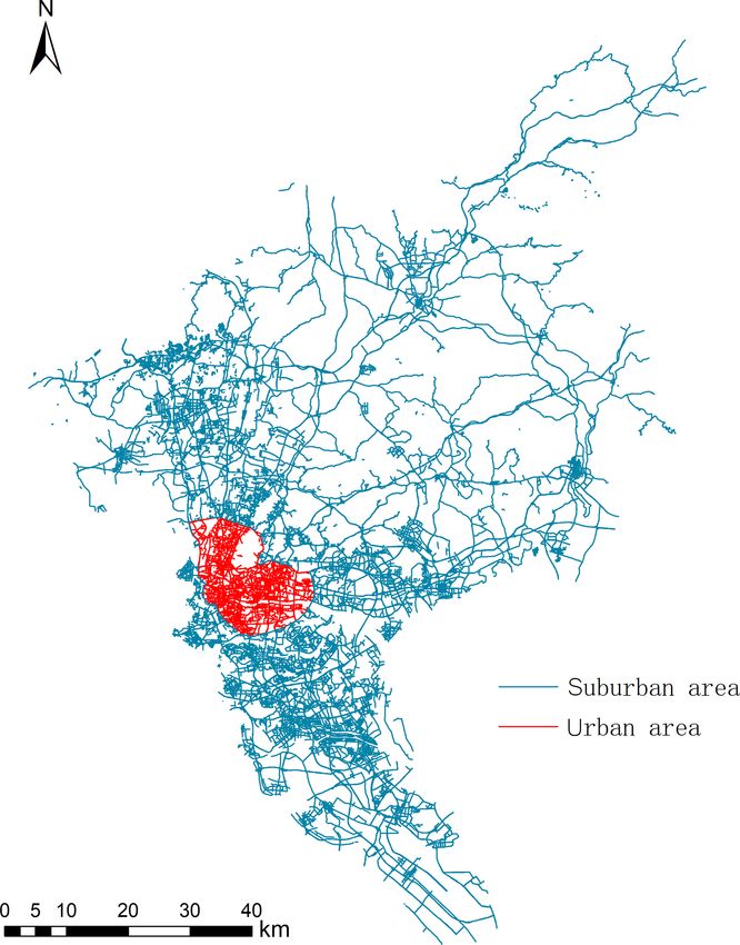
Given Guangzhou’s traffic control policies, the whole city which were representative of the street network.
is divided into two areas: urban area and suburban (Fig. 3). The urban morphology data for the building height were
Therefore, the traffic volume is also calculated accordingly obtained from the World Urban Database and Access Por-
(Fig. 4). The main traffic control policies in urban areas are tal Tools (WUDAPT) dataset (Ching et al., 2018). The street
as follows: (1) no truck is allowed to enter the urban area dur- data were sourced from the OpenStreetMap dataset (https:
ing 07:00–09:00 LT (all times in this paper are local time, LT) //www.openstreetmap.org/, last access: 2 September 2019).
(morning rush hours) and 18:00–20:00 (evening rush hours), The street length data were calculated directly from the loca-
(2) no middle- and heavy-duty truck is permitted to enter the tions of the start and end intersections of each street segment.
urban area during 07:00–22:00, (3) no nonlocal truck can en- Data on the street width were retrieved from the feature class
ter the urban area during 07:00–22:00, and (4) no motorcycle of the road and the width of each lane was assumed to be
can enter the urban area. 3.5 m.
The simulation period of the study spanned from 28 April
2.5 Vehicle fleet information to 2 May 2018, which included a Chinese national holiday
from 29 April to 1 May 2018. Significant traffic volume
In this study, the fleet information on each vehicle classifica- change exists between the holidays and nonholidays. This
tion was sourced from the Guangzhou Statistical Yearbook simulation period covered holidays and nonholidays, which
(Guangzhou Bureau of Statistics, 2017) (Fig. 5a). The emis- was helpful to investigate the impact of traffic volume varia-
sion standards (Fig. 5b) and fuel type data (Fig. 6) for the tions on air quality. Another 3 d simulation period was con-
vehicles were sourced from previous studies undertaken in ducted before this period to spin up the model.
Guangzhou (Zhang et al., 2013, 2015). Due to the lack of For modeling evaluation and background concentrations,
street-level vehicle fleet information, this study used a uni- the observational concentration data for NO2 and O3 were
form percentage of emission standard, fuel type, and number obtained from the Guangzhou environmental monitoring
of vehicles in each category for each segment. The number sites network. NO2 concentrations were measured with a
of each vehicle type was calculated based on the total traffic chemiluminescence instrument (model 42i, Thermo Scien-
volume of each street segment and the vehicle fleet percent- tific) and O3 was measured by a UV photometric ana-
age. It should be noted that this information could be updated lyzer (model 49i, Thermo Scientific). The minimum detec-
if the street-level fleet information becomes available in the tion limit (3S/N) of the analyzer was 0.4 ppbV (approxi-
future. mately 0.8 µg m−3 ) for NO2 and 1.0 ppbV (approximately
www.geosci-model-dev.net/13/23/2020/ Geosci. Model Dev., 13, 23–40, 2020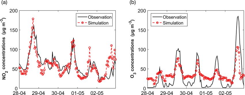
28                                         L. Wu et al.: Development of the Real-time On-road Emission (ROE v1.0) model

Figure 2. Traffic information from Gaode Map (© 2019).

Table 1. Physical parameterization configurations for WRF v3.7.1 model.

                     Physical parameterizations
                     Microphysics scheme           Morrison (2 moments) (Morrison et al., 2009)
                     Land-surface scheme           Pleim–Xiu (Xiu and Pleim, 2001)
                     Cumulus scheme                Kain–Fritsch (Kain, 2004)
                     Longwave radiation scheme     Rapid Radiative Transfer Model (RRTM) (Mlawer et al., 1997)
                     Shortwave radiation scheme    Dudhia (Dudhia, 1989)
                     Boundary-layer scheme         Asymmetric Convective Model version 2 (ACM2) (Pleim, 2007)
                     Urban surface scheme          Urban Canopy Model (UCM) (Chen et al., 2011)

2.0 µg m−3 ) for O3 . The total measurement uncertainty in           road vehicles from the ROE model was established for this
these two instruments was estimated to be approximately 5 %          study. Table 2 shows the annual emissions from vehicles
(Zhang et al., 2014).                                                in Guangzhou city compared with two other gridded emis-
   Two monitoring sites, Tiyuxi (TYX) site and YangJi (YJ)           sion inventories in China: the MEIC model (http://www.
site, were selected for this study (Fig. 7c). The observational      meicmodel.org/, last access: 2 September 2019) and a PRD
data from TYX were used for modeling evaluation because              region local emission inventory (Zheng et al., 2009b). These
TYX is located inside the simulation area and thus these data        two emission inventories used the top-down method to es-
could be used for comparison with the model results. In ad-          tablish on-road emission inventories. Unlike the bottom-up
dition, YJ is located near but not within the simulation street      method used in this study, these two inventories first calcu-
network. The observational data from YJ could be used as             lated the total emissions based on the VKT data of vehicle
the background concentration data for the modeling. Due to           categories. In the MEIC inventory, the total number of vehi-
the lack of NO observational data, the concentration ratio of        cles was obtained from the relationship between total vehicle
NO2 to NO was assumed as 4 : 1 in this study.                        ownership and economic development (Zheng et al., 2014),
                                                                     while the PRD inventory acquired information on the number
                                                                     of vehicles from the city-level Guangzhou Statistical Year-
4     Application of the ROE model to Guangzhou                      book. Then, the spatial distribution of these two inventories
                                                                     was established based on the road network density.
4.1     On-road emission inventory from the ROE model                   Given the shorter total road length and traffic control poli-
                                                                     cies in urban areas (Fig. 3), the urban on-road emissions of
4.1.1    Overview of the emission inventory                          CO, NOx , HC, PM2.5 , and PM10 comprised only 13.1 %,
                                                                     8.8 %, 12.7 %, 8.2 %, and 9.1 % of the total on-road emis-
Using the high-resolution spatial and temporal traffic data
from the map application, the emission inventory of on-

Geosci. Model Dev., 13, 23–40, 2020                                                      www.geosci-model-dev.net/13/23/2020/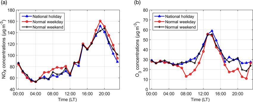
L. Wu et al.: Development of the Real-time On-road Emission (ROE v1.0) model 29
tor of an LPG-fueled bus is 1.7 times that of a diesel-fueled
bus in Guangzhou (Zhang et al., 2013). The results in Fig. 8
show that the NOx emissions attributable to buses in urban
and suburban areas were 20.5 % and 10.8 % of the total NOx
emissions, respectively, showing that the LPG-fueled buses
may be responsible for higher NOx estimates in this study
compared to those in the other two inventories.
As shown in Table 3, the emission contribution of lo-
cal roads in urban areas is the highest component because
of the total length of the local roads, which is 5.4 times
and 4.8 times that of highways and arterial roads in urban
areas, respectively. Although the total length of the high-
ways is shorter, the traffic volume on the highway is much
higher than that on the local roads (Fig. 4), thus caus-
ing the highest contribution of emissions from the subur-
ban areas. Moreover, the emission contributions from ur-
ban and suburban areas differ on weekdays and week-
ends. In urban areas, the daily total weekday and week-
end emissions are 129.94 and 118.29 Mg d−1 of CO, 30.15
and 27.71 Mg d−1 of NOx , 14.74 and 13.40 Mg d−1 of HC,
1.27 and 1.16 Mg d−1 of PM2.5 , and 1.41 and 1.29 Mg d−1
of PM10 , respectively. In suburban areas, the total week-
day and weekend emissions are 873.97 and 758.41 Mg d−1
of CO, 315.10 and 267.91 Mg d−1 of NOx , 102.46 and
88.22 Mg d−1 of HC, 13.01 and 10.98 Mg d−1 of PM2.5 , and
14.45 and 12.19 Mg d−1 of PM10 , respectively. The total
respective emissions of CO, NOx , HC, PM2.5 , and PM10
Figure 3. Traffic control area. on a weekday are 114.5 %, 116.8 %, 115.3 %, 117.6 %, and
117.7 % of the values on a weekend, respectively.
Table 2. Annual on-road emissions in Guangzhou (unit:
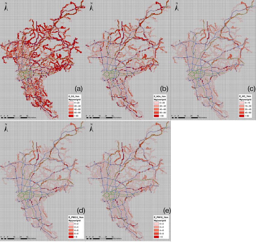
104 Mg yr−1 ). 4.1.2 Spatial distribution of emissions
CO NOx HC PM2.5 PM10 Due to the vehicular activities, the spatial distribution of on-
Urban 4.61 1.07 0.52 0.04 0.05 road emissions was consistent with the structure of the street
This study Suburban 30.61 10.98 3.58 0.45 0.50 network. For a better description of this spatial distribution,
Total 35.22 12.05 4.10 0.49 0.55
the emissions were mapped onto a 1 km resolution fishnet
pattern and the total emissions of one grid cell were the sum
MEIC-2016 (Gridded) 43.56 8.45 9.26 0.46 0.47 of all on-road emissions from within the same grid cell. The
PRD-2015 (Gridded) 28.89 6.99 4.65 0.52 0.52
spatial distribution of each pollutant is shown in Fig. 9. Over-
all, the high-value grid cells were generally located along the
highways. In suburban areas, high-value areas located away
sions, respectively, suggesting that the suburban areas are the from the highways and arterial roads normally denoted sub-
dominant contributor to on-road emissions in Guangzhou. urban town centers that had more local roads and higher traf-
In general, the difference between the amounts of PM2.5 fic volume density. In urban areas, the high-value areas were
and PM10 was smaller than that for other gaseous emissions more closely related to the densities of the urban local roads.
among different inventories. This was because the uncer- The emission hotspots were less prominent in urban areas
tainty in particulate matter emission factors was lower than than in suburban areas due to the strict traffic control policies
the corresponding values of the other gaseous emissions, in urban area. The spatial distribution indicated that the next
which led to the large difference for the gaseous emissions on-road emissions control policy should pay more attention
and the smaller differences for PM2.5 and PM10 . For NOx to the control of vehicles in suburban areas.
emissions, however, this study showed a higher NOx esti- Moreover, the spatial distributions of these three emission
mate than those in the other two inventories. One of the rea- inventories were compared in this study. Figure 10 shows the
sons for the higher NOx estimate may be the application of distributions of CO from the three different inventories. The
the updated LPG bus emission factors in this study. Based on results of both MEIC-2016 and PRD-2015 showed the ur-
a previous local emission factor study, the NOx emission fac- ban areas as emission hotspots. However, the results from
www.geosci-model-dev.net/13/23/2020/ Geosci. Model Dev., 13, 23–40, 2020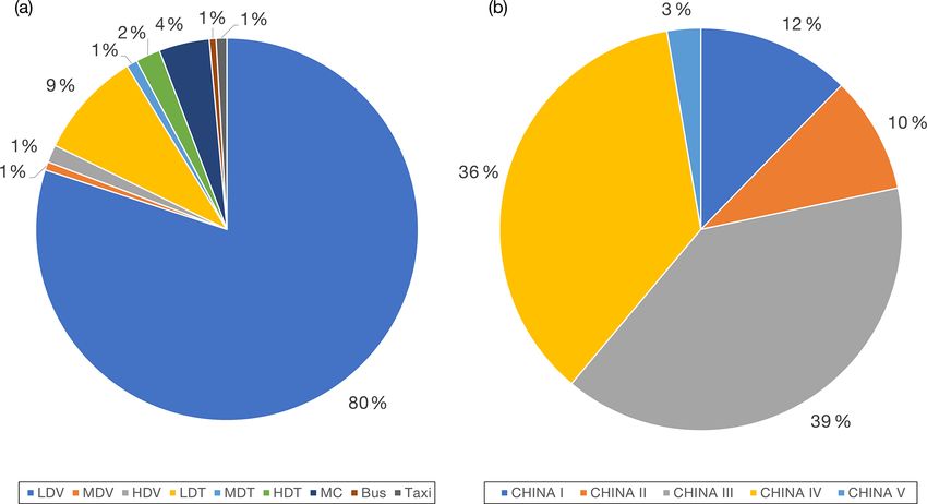
30                                           L. Wu et al.: Development of the Real-time On-road Emission (ROE v1.0) model

Figure 4. Diurnal variation in average traffic speed and traffic volume in (a, b) urban area and (c, d) suburban area during weekday and
weekend.

Figure 5. The percentage of (a) vehicle classification and (b) emission standard.

Geosci. Model Dev., 13, 23–40, 2020                                                         www.geosci-model-dev.net/13/23/2020/
L. Wu et al.: Development of the Real-time On-road Emission (ROE v1.0) model 31
Table 3. Daily emissions on different road types in urban and suburban areas (unit: Mg d−1 ).
Road type Length (km) CO NOx HC PM2.5 PM10
Weekday urban highway 301.87 9.71 3.15 1.02 0.11 0.12
artery 337.19 17.24 4.95 1.88 0.19 0.21
local 1629.92 102.99 22.05 11.84 0.97 1.08
suburban highway 2316.73 417.49 168.29 45.51 6.50 7.22
artery 747.63 61.12 26.54 7.24 1.11 1.23
local 8867.69 395.36 120.27 49.71 5.40 6.00
Weekend urban highway 301.87 7.47 2.34 0.79 0.08 0.09
artery 337.19 13.20 4.23 1.40 0.15 0.17
local 1629.92 97.62 21.14 11.21 0.93 1.03
suburban highway 2316.73 428.30 156.78 47.14 6.07 6.74
artery 747.63 59.20 26.56 6.99 1.10 1.22
local 8867.69 270.91 84.57 34.09 3.81 4.23
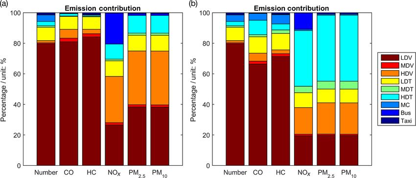
were the second largest contributor to on-road emissions, the
relevant percentages being 5.8 %, 2.9 %, 30.3 %, 35.2 %, and
35.2 % for CO, HC, NOx , PM2.5 , and PM10 , respectively. As
for the buses, except for the contribution of NOx which ac-
counted for 20.5 % of the total emissions mentioned above,
the proportions of the other pollutants were less than 2 % be-
cause of the use of LPG as fuel. In the case of trucks, the total
contribution of LDTs, MDTs, and HDTs were 10.3 %, 9.3 %,
21.2 %, 23.3 %, and 23.3 % for CO, HC, NOx , PM2.5 , and
PM10 , respectively, considering the traffic control policies in
the urban areas. The contribution of taxis was less than 1 %
because of the small number of taxis and their use of LPG.
In suburban areas, the LDVs were the dominant contribu-
tor of CO and HC emissions because of their high numbers.
For NOx , PM2.5 , and PM10 , however, the HDT provided the
largest contribution at 36.5 %, 43.2 %, and 43.3 %, respec-
Figure 6. Fuel type percentage of each vehicle classification. tively. Moreover, LDVs, HDVs, and buses were important
contributors of NOx at 19.4 %, 17.4 %, and 10.8 %, respec-
tively. Regarding particulate matter, the respective percent-
the ROE model were much lower for such areas. This may ages of emissions (for both PM2.5 and PM10 ) owing to LDVs,
be due to the fact that the ROE model considers the traffic HDVs, and LDTs were 19.7 %, 20.5 %, and 9.0 %, suggest-
control policies, while the other two inventories do not. In ing that these vehicles were also important sources of both
suburban town centers, especially in the eastern and southern PM2.5 and PM10 .
parts of Guangzhou, all three inventories showed the same
results, namely that these areas were large contributors of 4.2 Application of the ROE model’s results to the
on-road emissions. Notably, highways and arterial roads also street-level air quality model
contributed high emissions in all three inventories.
4.1.3 Emission contributions of vehicles by their 4.2.1 Modeling performance in Guangzhou urban area
classification
During the simulation period, the model results were evalu-
The emission contributions of different vehicle classifica- ated for the TYX observation site located within the street
tions in the urban and suburban areas are shown in Fig. 8. As network. The on-road emissions were provided by the ROE
LDVs accounted for the largest number, their emission con- model, as discussed previously. Street segments to which
tribution comprised the dominant proportion of total emis- high NOx emission values were attributed were also respon-
sions in urban areas for each pollutant. The contribution per- sible for high HC emissions because of the positive relation-
centages of CO, HC, NOx , PM2.5 , and PM10 were 80.9 %, ship between traffic volume and on-road emissions as shown
84.1 %, 26.4 %, 38.3 %, and 38.2 %, respectively. HDVs in Fig. 11.
www.geosci-model-dev.net/13/23/2020/ Geosci. Model Dev., 13, 23–40, 202032 L. Wu et al.: Development of the Real-time On-road Emission (ROE v1.0) model Figure 7. Simulation domain from regional scale to street-level scale: (a) four times nested simulation for WRF; (b) domains 3 and 4 covering the Pearl River Delta region and Guangzhou city, the innermost box corresponds to the Tianhe District; (c) 31 street segments and two observation sites (triangles) within the MUNICH study domain. Figure 8. Emission contribution of each vehicle classification in (a) urban area and (b) suburban area. The time series for the simulated NO2 and O3 concen- servation (OBS) mean, simulation (SIM) mean, mean bias trations within the street network were compared with the (MB), normalized mean bias (NMB), normalized mean er- observed concentrations (Fig. 12). As the results show, day- ror (NME), mean relative bias (MRB), mean relative error time NO2 concentrations were overestimated while night- (MRE), root-mean-squared error (RMSE), and the correla- time concentrations were underestimated during the simula- tion coefficient (CORR) were used to validate the model. The tion period. The O3 concentrations, however, were underpre- NMB, NME, and CORR values of NO2 and O3 in this study dicted during daytime and overpredicted at nighttime. Sev- were within the recommended ranges in the MEP Technical eral modeling sensitivity cases were analyzed to identify Guide for Air Quality Model Selection (MEP, 2012). These what factors may have affected the model simulation. The recommended values were −40 % < NMB < 50 %, NME < sensitivity analysis results are provided in the Supplement 80 %, and R 2 > 0.3 for NO2 and −15 % < NMB < 15 %, Sect. S3. Typically, the overestimated background concen- NME < 35 %, and R 2 > 0.4 for O3 . Additionally, the values trations of NO2 and O3 were attributed as the reason for the obtained in this study fell within the range of those reported overprediction of the daytime NO2 and nighttime O3 concen- by other modeling studies in Guangzhou; the NMB, NME, trations, respectively. The underestimated NO titration was and RMSE values for simulated urban NO2 in Guangzhou the other main reason for the overprediction of O3 and the un- ranged from −27.5 % to −6 %, 29.2 % to 53.0 %, and 16 to derprediction of NO2 concentrations at night. Due to the only 37.3, respectively, and the corresponding ranges for O3 were consideration of on-road emission in the simulation street from −21.2 % to 20.0 %, 38.2 % to 98 %, and 9.4 to 40.1 network, daytime O3 concentrations were underpredicted in (Che et al., 2011; Fan et al., 2015; Wang et al., 2016). Over- the results. all, the model showed good simulation performance and can Moreover, the performance statistics for NO2 and O3 are be applied to future studies investigating the impact of on- shown in Table 4. Here, the statistical measures of the ob- road vehicles on air quality. Geosci. Model Dev., 13, 23–40, 2020 www.geosci-model-dev.net/13/23/2020/
L. Wu et al.: Development of the Real-time On-road Emission (ROE v1.0) model                                                          33

Figure 9. Spatial distribution of (a) CO, (b) NOx , (c) HC, (d) PM2.5 , and (e) PM10 from the on-road emissions in Guangzhou (blue lines:
highways; green lines: arterial roads; local roads are not shown).

Figure 10. Spatial distribution of CO from (a) ROE model, (b) MEIC-2016, and (c) PRD-2015 in Guangzhou.

www.geosci-model-dev.net/13/23/2020/                                                           Geosci. Model Dev., 13, 23–40, 2020
34                                           L. Wu et al.: Development of the Real-time On-road Emission (ROE v1.0) model

Figure 11. The spatial distribution of weekday (a) NOx and (b) HC emissions in the simulated street network.

Figure 12. Time series of (a) NO2 and (b) O3 during the simulation period. (solid black line: observation; dashed red line: simulation).

4.2.2   Impact of traffic volume variations on air quality

To investigate how traffic volume change affects air quality
at the street level, a Chinese national holiday was chosen
as the target simulation period for the modeling. Figure 13
shows the diurnal variation in the traffic volume during the
national holiday, normal weekday, and normal weekend be-
fore and after the holiday in the simulation street network. On
the normal weekday, two typical rush hour trends appeared
during the 08:00–10:00 and 17:00–19:00 periods (although
28 April was a Saturday, it was a normal workday to com-
pensate for the holiday). For the normal weekend and the
national holiday, the peak in traffic volume was noted be-
tween 14:00 and 16:00 and no rush hour peak occurred on
these days. At nighttime, not much difference was noted for
the traffic volumes on the normal weekday, normal weekend,
and national holiday, especially after midnight. However, the            Figure 13. The diurnal variation in the total traffic volume in the
higher traffic volume between 21:00 and 23:00 on 28 April                simulation street network (solid line: normal weekday; dashed line:
at night may have been caused by people traveling out of the             national holiday; dotted line: normal weekend).
city before the national holiday (e.g., returning home across
the city or traveling to other places).
   Three sensitivity cases were carried out to study the impact          sions between 29 April and 1 May were regarded as the orig-
of traffic volume change on the air quality in urban areas:              inal emissions during the simulation period (this represents
(1) in the national holiday case, wherein the on-road emis-              the base case); (2) in the normal weekday case, diurnal on-

Geosci. Model Dev., 13, 23–40, 2020                                                            www.geosci-model-dev.net/13/23/2020/
L. Wu et al.: Development of the Real-time On-road Emission (ROE v1.0) model                                                                       35

Table 4. The performance statistics for NO2 and O3 in modeling (unit: µg m−3 ).

                                    Mean
                               OBSa       SIMb        MBc        NMBd         NMEe           MRBf        MREg        RMSEh         CORRi
                     NO2         30.8       35.4      4.7       15.2 %        68.8 %        3.0 %         3.2 %           25.7         0.90
                     O3          60.9       59.3     −1.6       −2.7 %        24.3 %      < 0.1 %         0.3 %           18.7         0.80
                   a OBS (observation). b SIM (simulation). c MB (mean bias). d NMB (normalized mean bias). e NME (normalized mean error).
                   f MRB (mean relative bias). g MRE (mean relative error). h RMSE (root-mean-squared error). i CORR (correlation coefficient).

road emissions for three national holidays were replaced by                         5    Discussion and conclusions
the emissions of 28 April; and (3) in the normal weekend
case, the national holiday period emissions were replaced by                        Using real-world traffic information, the Real-time On-road
the diurnal on-road emissions of 5 May. The diurnal varia-                          Emission (ROE v1.0) model can provide real-time and high-
tions in NOx and O3 in the three cases are shown in Fig. 14.                        resolution emission inventories for regional or street-level
During 00:00–05:00, because of similar traffic volume, there                        air quality models in China. The results show that the ROE
were no large differences in the NOx and O3 concentrations                          model can simulate the emissions of CO, NOx , HC, PM2.5 ,
during this time. Due to the morning rush hour, the NOx con-                        PM10 , and any other pollutant provided the relevant emis-
centrations for the normal weekday case were much higher                            sion factors are included in the model. (This aspect will
than those for the national holiday case in the morning. As                         be updated in subsequent releases.) As it uses the bottom-
shown in Table 5, the NOx concentrations were 12.0 %–                               up method, the ROE model facilitates the calculation of the
26.5 % higher for the normal weekday case during this time.                         emissions in each street segment.
In the normal weekend case too, the NOx concentrations si-                             In this study, the traffic information of Guangzhou was
multaneously increased by 9.1 % compared to those on the                            obtained from the Gaode Map, the data for which are col-
national holiday in the morning. This increase was caused                           lected from map users while they are driving. The geographic
by people traveling for normal weekend engagements. In the                          and speed information were sourced from the map users’
afternoon, however, the difference between the NOx concen-                          GPS devices and can be used through the map API. Us-
trations was less than 10 % due to the rising traffic volume                        ing the ROE model and fully considering the traffic control
on the national holiday. During the evening rush hour, al-                          policies of Guangzhou city, the annual total on-road emis-
though the traffic volume on the normal weekday was 1.3                             sions of CO, NOx , HC, PM2.5 , and PM10 were modeled
times that on the national holiday, the maximum difference                          to be 35.22 × 10⁴ , 12.05 × 10⁴ , 4.10 × 10⁴ , 0.49 × 10⁴ , and
between the NOx concentrations was only 7.3 %. This shows                           0.55 × 10⁴ Mg yr−1 , respectively. Spatial distribution analy-
that the variations in NOx concentrations were affected to a                        sis showed that hotspots of on-road emissions were situated
greater extent by the background concentrations (i.e., bound-                       along the highways and suburban town centers. The com-
ary conditions) in the evening.                                                     parison of spatial distribution between the ROE model’s re-
   Compared with the national holiday case, the O3 concen-                          sults and those of two other inventories showed that the ROE
trations were much lower in the normal weekday case. In the                         model provided lower urban emissions as it considered the
afternoon, as shown in Table 6, when photochemical reac-                            traffic control polices. However, it should be noted that this
tions are more prevalent, the national holiday O3 concentra-                        comparison was only preliminary. The spatial resolutions of
tions exceeded those on normal weekdays and weekends by                             the three inventories are inconsistent in this study. Moreover,
13.9 % and 10.6 %, respectively. This is because the simula-                        due to the lack of temporal information about the other two
tion street network in the urban areas is in the VOC-sensitive                      emission inventories, a comparison of the temporal differ-
(volatile organic compound) regime (Ye et al., 2016). The                           ence could not be conducted. Future studies should focus on
O3 concentrations were positively correlated with the VOC                           improving the accuracy of such comparisons.
emissions. As the NOx emissions were higher than the VOC                               Owing to the number of vehicles and their respective dis-
emissions, the reduction in the NOx emissions was also much                         tributions, LDVs constituted the dominant source of on-road
higher than in the VOC emissions when the number of vehi-                           emissions in Guangzhou. In suburban areas, however, HDTs
cles decreased on the national holiday. The larger NOx emis-                        were the highest contributors of NOx , PM2.5 , and PM10 .
sion reduction led to a higher VOCs-to-NOx emission ratio,                          Daily emissions of CO, NOx , HC, PM2.5 , and PM10 on a
which resulted in a higher O3 concentration during the na-                          weekday were found to be 14.5 %, 16.8 %, 15.3 %, 17.6 %,
tional holiday (Sanford and He, 2002).                                              and 17.7 % higher than the daily emissions on a weekend,
                                                                                    respectively. However, due to the lack of street-level vehicle
                                                                                    fleet information, this study applied a city-level average uni-
                                                                                    form percentage for every street segment. This may increase

www.geosci-model-dev.net/13/23/2020/                                                                               Geosci. Model Dev., 13, 23–40, 2020
36 L. Wu et al.: Development of the Real-time On-road Emission (ROE v1.0) model Table 5. Daytime percentage difference of NOx compared to national holiday case. Time 06:00 07:00 08:00 09:00 10:00 11:00 12:00 13:00 14:00 15:00 16:00 17:00 18:00 19:00 20:00 Normal weekday 12.7 21.7 16.8 26.5 14.7 12.0 4.9 0.6 8.6 2.2 0.7 0.2 7.3 5.9 7.1 Normal weekend −4.4 0.1 9.1 6.7 0.2 7.0 1.2 2.6 6.2 0.8 −0.6 −0.9 2.1 −5.7 4.9 Table 6. Daytime percentage difference of O3 compared to national holiday case. Time 06:00 07:00 08:00 09:00 10:00 11:00 12:00 13:00 14:00 15:00 16:00 17:00 18:00 19:00 20:00 Normal weekday −4.5 −15.7 −52.8 −48.9 −37.5 −25.9 −15.6 0.2 −7.9 −13.9 −7.4 −11.1 −46.3 −38.4 −32.3 Normal weekend 2.9 6.3 −2.6 −4.9 −15.0 0.5 −4.0 −1.6 −5.7 −10.6 −0.4 12.4 −15.3 −0.1 3.7 Figure 14. The (a) NOx and (b) O3 diurnal variation in different sensitivity cases in the simulation street network. the uncertainty in the inventory but this aspect can be im- derstand the variations in street-level air quality in urban or proved upon, provided additional data become available in suburban areas of a megacity. The results of the ROE model the future. Given the high spatial and temporal resolutions of showed that the suburban town centers of Guangzhou served the emission inventory of the ROE model, three sensitivity as emission hotspots. These areas had relatively higher emis- cases were analyzed to study the effect of vehicular on-road sions than the other suburban areas and less stringent control emissions on urban street-level air quality. On a national holi- policies than the urban area, which suffers from more serious day, NOx concentrations were 12.0 %–26.5 % less than those air quality problems. on a normal weekday as no morning rush hours occurred on In general, the ROE model could provide a high-resolution holidays. Moreover, compared with the normal weekend, the on-road emission inventory when the real-time traffic infor- NOx concentrations on a national holiday also show a de- mation and emission factors were fed into the model. It is crease of 9.1 % in the peak value in the morning. However, worth noting that the ROE model is highly dependent on the the reduction in the NOx concentrations in the afternoon was ITS traffic data. For economically underdeveloped cities, this smaller than that in the morning, suggesting that the trans- aspect may pose a barrier against the use of the ROE model. portation of NOx from the surrounding areas was the main In addition, China is promoting the CHINA VI emission reason for the variation in the afternoon NOx concentrations. standards for on-road vehicles. The ROE model only con- In addition, as the simulation street network lies in the VOC- siders Pre-CHINA I to CHINA V currently. Thus, the model sensitive regime, the lower traffic on a national holiday and a will be updated in the near future to include the CHINA VI normal weekend caused the NOx and VOC emissions to be emission standards. lower than those on a normal weekday. However, the reduc- Recently studies had shown that traffic forecasting mod- tions in NOx were higher than the decrease in VOC emis- els are effective within cities (Min et al., 2009; Cortez et al., sions, which led to a higher VOC-to-NOx emission ratio and 2012; Vlahogianni et al., 2014). These models allow one to O3 concentrations on holidays and normal weekends. In this obtain predicted traffic-based on-road emissions. Combined study, only 31 main street segments were selected to study with the meteorological forecasting systems and regional air the impact of a holiday on air quality in a certain urban area quality forecasting systems, which provide the meteorolog- of Guangzhou. Additional investigations are required to un- ical and background concentration predictions, respectively, Geosci. Model Dev., 13, 23–40, 2020 www.geosci-model-dev.net/13/23/2020/
L. Wu et al.: Development of the Real-time On-road Emission (ROE v1.0) model                                                             37

street-level air quality models could be used for street-level         References
air quality forecasting as well.
   In summary, the newly developed ROE model was con-                  An, X., Hou, Q., Li, N., and Zhai, S.: Assessment of human ex-
firmed to be effective for analyzing real-time city-scale traffic        posure level to PM10 in China, Atmos. Environ., 70, 376–386,
                                                                         https://doi.org/10.1016/j.atmosenv.2013.01.017, 2013.
emissions and performing high-resolution air quality assess-
                                                                       Ashie, Y. and Kono, T.: Urban-scale CFD analysis in support of a
ments in the street networks of Guangzhou city. The method-              climate-sensitive design for the Tokyo Bay area, Int. J. Climatol.,
ologies presented in this work can be further extended to                31, 174–188, https://doi.org/10.1002/joc.2226, 2011.
more typical cities, urban districts in China, or other coun-          Britter, R. E. and Hanna, S. R.: Flow and dispersion in
tries.                                                                   urban areas, Annu. Rev. Fluid Mech., 35, 469–496,
                                                                         https://doi.org/10.1146/annurev.fluid.35.101101.161147, 2003.
                                                                       Cai, H. and Xie, S. D.: Estimation of vehicular emission inventories
Code availability. The python source code of the ROE v1.0 model          in China from 1980 to 2005, Atmos. Environ., 41, 8963–8979,
and examples are available on GitHub (https://github.com/vnuni23/        https://doi.org/10.1016/j.atmosenv.2007.08.019, 2007.
ROE, last access: 2 September 2019) and Zenodo (https://doi.org/       Che, W., Zheng, J., Wang, S., Zhong, L., and Lau, A.: Assessment
10.5281/zenodo.3264859, Wu, 2019). More information and help             of motor vehicle emission control policies using Model-3/CMAQ
are also available by contacting the authors.                            model for the Pearl River Delta region, China, Atmos. Environ.,
                                                                         45, 1740–1751, https://doi.org/10.1016/j.atmosenv.2010.12.050,
                                                                         2011.
Supplement. The supplement related to this article is available on-    Chen, F., Kusaka, H., Bornstein, R., Ching, J., Grimmond, C. S.
line at: https://doi.org/10.5194/gmd-13-23-2020-supplement.              B., Grossman-Clarke, S., Loridan, T., Manning, K. W., Martilli,
                                                                         A., Miao, S., Sailor, D., Salamanca, F. P., Taha, H., Tewari, M.,
                                                                         Wang, X., Wyszogrodzki, A. A., and Zhang, C.: The integrated
Author contributions. LW and XW designed the experiments. LW             WRF/urban modelling system: development, evaluation, and ap-
developed the model code and performed the simulations. MC or-           plications to urban environmental problems, Int. J. Climatol., 31,
ganized and visualized the data. JZ collected and organized the ob-      273–288, https://doi.org/10.1002/joc.2158, 2011.
servational data. LW and JH prepared the article with contributions    Chen, R., Paristech, P., and Aguil, V.: A sensitivity study of road
from all coauthors. LW organized the results of model sensitivity        transportation emissions at metropolitan scale, J. Earth Sci.
cases. XW and MS proposed revision suggestions for the article.          Geotech. Eng., 7, 151–173, 2017.
                                                                       Ching, J., Mills, G., Bechtel, B., See, L., Feddema, J., Wang,
                                                                         X., Ren, C., Brorousse, O., Martilli, A., Neophytou, M.,
                                                                         Mouzourides, P., Stewart, I., Hanna, A., Ng, E., Foley, M.,
Competing interests. The authors declare that they have no conflict
                                                                         Alexander, P., Aliaga, D., Niyogi, D., Shreevastava, A., Bha-
of interest.
                                                                         lachandran, P., Masson, V., Hidalgo, J., Fung, J., Andrade, M.,
                                                                         Baklanov, A., Dai, W., Milcinski, G., Demuzere, M., Brunsell,
                                                                         N., Pesaresi, M., Miao, S., Mu, Q., Chen, F., and Theeuwesits,
Acknowledgements. We acknowledge the technical support and               N.: WUDAPT: An urban weather, climate, and environmental
computational time from the Tianhe-2 platform at the National Su-        modeling infrastructure for the anthropocene, B. Am. Meteo-
percomputer Center in Guangzhou. We also thank Yang Zhang and            rol. Soc., 99, 1907–1924, https://doi.org/10.1175/BAMS-D-16-
Youngseob Kim for their helpful advice on the street-level air qual-     0236.1, 2018.
ity model.                                                             Cortez, P., Rio, M., Rocha, M., and Sousa, P.: Multi-scale Internet
                                                                         traffic forecasting using neural networks and time series meth-
                                                                         ods, Expert Syst., 29, 143–155, https://doi.org/10.1111/j.1468-
Financial support. This research has been supported by the Na-           0394.2010.00568.x, 2012.
tional Key Research and Development Program of China (grant            Davies, L., Bates, J. W., Bell, J. N. B., James, P. W., and
no. 2016YFC0202206), the National Nature Science Fund for Dis-           Purvis, O. W.: Diversity and sensitivity of epiphytes to ox-
tinguished Young Scholars (grant no. 41425020), the State Key            ides of nitrogen in London, Environ. Pollut., 146, 299–310,
Program of National Natural Science Foundation of China (grant           https://doi.org/10.1016/j.envpol.2006.03.023, 2007.
no. 91644215), and the National Natural Science Foundation–            Di Sabatino, S., Buccolieri, R., Pulvirenti, B., and Britter, R. E.:
Outstanding Youth Foundation (grant no. 41622502).                       Flow and pollutant dispersion in street canyons using FLU-
                                                                         ENT and ADMS-Urban, Environ. Model. Assess., 13, 369–381,
                                                                         https://doi.org/10.1007/s10666-007-9106-6, 2008.
Review statement. This paper was edited by David Topping and re-       Dudhia,     J.:    Numerical     Study     of     Convection     Ob-
viewed by two anonymous referees.                                        served during the Winter Monsoon Experiment Us-
                                                                         ing a Mesoscale Two-Dimensional Model, J. Atmos.
                                                                         Sci.,      46,     3077–3107,        https://doi.org/10.1175/1520-
                                                                         0469(1989)0462.0.CO;2, 1989.
                                                                       EPA: User’s Guide to MOBILE6.1 and MOBILE6.2: Mobile
                                                                         Source Emission Factor Model, EPA420-R-03-010, Washington,
                                                                         DC, USA, 2003.

www.geosci-model-dev.net/13/23/2020/                                                            Geosci. Model Dev., 13, 23–40, 2020
You can also read