Accretion in common envelope evolution
←
→
Page content transcription
If your browser does not render page correctly, please read the page content below
MNRAS 000, 000–000 (0000)                                             Preprint 10th May 2018               Compiled using MNRAS LATEX style file v3.0

                                              Accretion in common envelope evolution

                                              Luke Chamandy1? , Adam Frank1 †, Eric G. Blackman1 ‡, Jonathan Carroll-Nellenback1 ,
                                              Baowei Liu1 , Yisheng Tu1 , Jason Nordhaus2,3 , Zhuo Chen1 and Bo Peng1
                                              1 Department  of Physics and Astronomy, University of Rochester, Rochester NY 14618, USA
                                              2 National Technical Institute for the Deaf, Rochester Institute of Technology, NY 14623, USA
                                              3 Center for Computational Relativity and Gravitation, Rochester Institute of Technology, NY 14623, USA
arXiv:1805.03607v1 [astro-ph.SR] 9 May 2018

                                              10th May 2018

                                                                                     ABSTRACT
                                                                                     Common envelope evolution (CEE) is presently a poorly understood, yet critical, process
                                                                                     in binary stellar evolution. Characterizing the full 3D dynamics of CEE is difficult in part
                                                                                     because simulating CEE is so computationally demanding. Numerical studies have yet to
                                                                                     conclusively determine how the envelope ejects and a tight binary results, if only the binary
                                                                                     potential energy is used to propel the envelope. Additional power sources might be necessary
                                                                                     and accretion onto the inspiraling companion is one such source. Accretion is likely common
                                                                                     in post-asymptotic giant branch (AGB) binary interactions but how it operates and how its
                                                                                     consequences depend on binary separation remain open questions. Here we use high resolution
                                                                                     global 3D hydrodynamic simulations of CEE with the adaptive mesh refinement (AMR) code
                                                                                     AstroBEAR, to bracket the range of CEE companion accretion rates by comparing runs that
                                                                                     remove mass and pressure via a subgrid accretion model with those that do not. The results
                                                                                     show that if a pressure release valve is available, super-Eddington accretion may be common.
                                                                                     Jets are a plausible release valve in these environments, and they could also help unbind and
                                                                                     shape the envelopes.
                                                                                     Key words: binaries: close – accretion, accretion discs – stars: kinematics and dynamics –
                                                                                     hydrodynamics – methods: numerical

                                              1   INTRODUCTION                                                                      The binary central stars of several bipolar PNe are close enough
                                                                                                                              to imply that they, and likely many more PNe, experienced a com-
                                              Close binary star interactions lie at the heart of many interesting
                                                                                                                              mon envelope interaction phase. The ejection of the primary’s envel-
                                              and poorly-understood stellar astrophysical phenomena. Common
                                                                                                                              ope, which is expected to be a necessary consequence of CEE, will
                                              envelope evolution (CEE), whereby a binary pair rapidly inspiral as
                                                                                                                              likely play a pivotal role in the formation of PNe. Winds from the
                                              the secondary enters the outer layers of the primary, represents such
                                                                                                                              exposed primary core (a proto white dwarf) will be shaped by their
                                              a binary process that can lead to a variety of crucial phenomena in
                                                                                                                              inertial interaction with toroidal ejected envelope and this may be
                                              stellar evolution (Paczynski 1976; Iben & Livio 1993; Ivanova et al.
                                                                                                                              a fundamental mechanism for producing PN bipolar morphologies
                                              2013; De Marco & Izzard 2017).
                                                                                                                              (Jones & Boffin 2017, and references therein).
                                                    Binaries are, for example, likely needed to explain the ubi-
                                              quity of bipolar planetary nebulae (PNe) and pre-planetary nebulae                   For more massive binary stars, progenitors of gravitational
                                              (PPNe) (Soker 1994; Reyes-Ruiz & López 1999; Soker & Rappaport                  wave (GW) generating mergers likely pass through a CEE phase
                                              2000, 2001; Blackman et al. 2001; Balick & Frank 2002; Nordhaus                 (Kalogera et al. 2007; Ivanova et al. 2013; Belczynski et al. 2014).
                                              & Blackman 2006; Nordhaus et al. 2007; Witt et al. 2009). PNe col-              The black hole (BH)-BH and neutron star (NS)-NS sources of
                                              limated outflow momenta are much less kinematically demanding                   recent gravitational wave detections via the Laser Interferometer
                                              than those found in PPNe so far (Bujarrabal et al. 2001; Blackman               Gravitational-Wave Observatory (LIGO) (and other GW detectors)
                                              & Lucchini 2014; Sahai et al. 2017). If PNe are the evolved states              were most likely preceded by a CEE phase that set-up the conditions
                                              of PPNe, strongly (rather than weakly) interacting binaries and the             for mergers (e.g. Abbott et al. 2016, 2017a,b).
                                              associated modes of accretion may be essential to explain these high                  Although first proposed more than four decades ago (Paczyn-
                                              momenta (Blackman & Lucchini 2014).                                             ski 1976), much of the physics of CEE still remains uncertain. The
                                                                                                                              process involves inherently 3D fluid dynamics (and magnetic fields;
                                                                                                                              Nordhaus & Blackman 2006; Nordhaus et al. 2007) but early ana-
                                              ? lchamandy@pas.rochester.edu                                                   lytic formalisms for CEE employ simplified parameterizations for
                                              † afrank@pas.rochester.edu                                                      energy or angular momentum exchange/loss (Livio & Soker 1988;
                                              ‡ blackman@pas.rochester.edu                                                    de Kool 1990; Iben & Livio 1993; Nelemans et al. 2000; Webbink

                                              © 0000 The Authors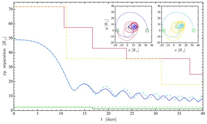
2      L. Chamandy et al.
2008; Ivanova et al. 2013). Numerical studies of CEE were, likewise,      two aforementioned cases highlights how very different conclusions
hampered by the need for both full 3D models and high resolution.         about CEE accretion can be reached depending on the presence or
      Early simulations of CEE include Rasio & Livio (1996);              absence of an inner loss valve.
Sandquist et al. (1998, 2000); Lombardi et al. (2006). Over the                 In Section 2 we describe our method. In Section 3 we present
last decade, more numerical codes have been adapted to study CEE.         results from the two aforementioned simulation cases, focusing on
These include both smoothed particle hydrodynamics (SPH) and              disk formation and accretion. In Section 4 we discuss the differences
grid-based (often adaptive or moving mesh) models. Beginning              that these two cases imply for the role of accretion in CEE, and
with Ricker & Taam (2008, 2012) and Passy et al. (2012) the com-          what is required to sustain accretion onto the companion. In Section
munity now has an expanding array of tools to study CEE. The              5 we summarize some numerical challenges and we conclude in
results are so far encouraging and puzzling. While the early inspiral     Section 6.
phase has been recovered in a variety of studies (Nandez et al. 2014;
Ohlmann et al. 2016; Staff et al. 2016; Kuruwita et al. 2016; Ivanova
& Nandez 2016; Iaconi et al. 2017, 2018) almost all models show
the orbital decay flattening out at distances too large to account        2     METHODS
for observations. Likewise the ejection of the envelope has proven
                                                                          2.1    Setup
difficult to achieve as much of the mass set in motion by the in-
spiral fails to reach the escape velocity and hence would tend to fall    We solve the equations of hydrodynamics for a binary system con-
back (Ohlmann et al. 2016; Kuruwita et al. 2016). This behavior is        sisting of a red giant (RG) and an unresolved stellar companion
seen in all models to date, and a number of explanations have been        represented by a (gravitation only) sink particle with mass equal
proposed. Mechanisms which allow the stars to continue to draw            to half of the RG mass. We adopt an ideal gas equation of state
closer may operate on longer timescales than the simulations (ie.         with adiabatic index γ = 5/3. Gravitational interactions between
thermal or stellar evolutionary timescales). Others have proposed         particles, and between particles and gas, as well as self-gravity
that mechanisms not included in the initial studies can drive the en-     of the gas, are calculated self-consistently. Although our numer-
velope away and allow the binary orbit to continue to shrink. Such        ical setup and chosen physical parameters follow closely those of
mechanisms include recombination (Nandez et al. 2015; Ivanova             Ohlmann et al. (2016, 2017) (hereafter ORPS16 and ORPS17, re-
& Nandez 2016) in the expanding/cooling envelope or radiation             spectively), the numerical methods are very different (e.g. our AMR
pressure on dust grains (Glanz & Perets 2018). The efficacy of such       vs. their moving mesh). In particular, our RG model and setup is
mechanisms remains strongly debated (e.g. Grichener et al. 2018).         very similar to theirs with a few minor differences discussed below.
      Accretion in CEE is of interest both because it may have a role     The similarity was deliberate because this RG setup resulted in a
in the envelope ejection and also because it is a ubiquitous engine for   star very close to hydrostatic equilibrium and enables a consistency
outflows (Frank et al. 2002). As discussed above, such outflows are       check between our independently obtained results and theirs.
prevalent in PPNe and PNe but have also been considered as a means              The reader is referred to ORPS17 for details, but we sum-
for driving some types of supernova (Milosavljević et al. 2012;           marize the procedure and notable differences between the two ap-
Gilkis et al. 2016). If such outflows occur during common envelopes       proaches below. We first evolve a star with a zero-age main sequence
(CEs) either via accretion onto the primary core (Blackman et al.         (MS) mass of 2M using the 1D stellar evolution code MESA (ver-
2001; Nordhaus et al. 2011) or onto the secondary, the evolution          sion 8845) (Paxton et al. 2011, 2013, 2015), setting the metallicity
may be altered and perhaps drive more of the envelope to escape           Z to 0.02, and select the snapshot that most closely coincides with
velocity. Some previous studies attempted to characterize accretion       the RG of ORPS16; ORPS17 on the Hertzsprung-Russell diagram.
in CEE simulations as part of global AMR simulations (Ricker &            We call this star the “primary” and its companion the “secondary.”
Taam 2008, 2012), and in “wind tunnel” formulations (MacLeod                    Numerically resolving the pressure scale-height in the core
& Ramirez-Ruiz 2015b; MacLeod et al. 2017). They found that               is unfeasible. We therefore truncate the RG at a radius r = rc =
accretion did occur with rates that were below that of Bondi-Hoyle-       2.41R , and replace the core by the combination of a gravitation-
Littleton (BHL) flows (Hoyle & Lyttleton 1939; Bondi & Hoyle              only sink particle and a surrounding density profile which smoothly
1944; Bondi 1952, see Edgar 2004 for a review), but still super-          matches the density at rc . The modified profile is obtained by numer-
Eddington. Murguia-Berthier et al. (2017) also used a “wind tunnel”       ically solving a modified Lane-Emden equation, with polytropic in-
formulation to explore CEE accretion and found that for lower values      dex n = 3, taking into account the gravitation of the sink particle and
of the polytropic index γ accretion discs could form.                     boundary conditions for ρ and dρ/dr. This particle is the “primary
      In this work we introduce and use a new tool to carry out           particle” and the remainder of the RG is the “primary envelope.”
CEE simulations, with a particular focus on accretion around the          Their masses are m1 (primary particle) and m1,env (primary en-
secondary. Using our AMR MHD multi-physics code AstroBEAR                 velope) where the total primary mass M1 = m1 + m1,env . Unlike
(Cunningham et al. 2009; Carroll-Nellenback et al. 2013),1 we have        in ORPS16; ORPS17, where m1 is set equal to the interior mass
developed modules for simulating CEE and here we describe our             m(rc ) of the MESA profile, we iterate over m1 , solving the equa-
initial results following the inspiral of a red giant branch (RGB)        tion at each iteration until m1 + m1,env (rc ) = m(rc ), where m(r)
star and a smaller companion. We present results from two high-           is the interior mass and m1,env (rc ) is the interior gas mass of the
resolution simulations, one of which uses a subgrid module for            modified profile. This prevents the mass of the modified RG from
accretion onto the “sink particle” secondary star that removes mass       exceeding that of the original MESA model and, more importantly,
and pressure (Krumholz et al. 2004) (hereafter, KMK04), and the           maintains a higher degree of hydrostatic equilibrium in the RG than
other without a subgrid model. Both cases show general features of        would have otherwise obtained. The initial mass and radius of the
the inspiral but a dramatic difference in accretion rates between the     primary are M1 = 1.956M and R1 = 48.1R , respectively, with
                                                                          m1 = 0.369M .
                                                                                Simulations are carried out in the inertial centre of mass frame,
1  For a discussion of angular momentum conservation in AstroBEAR, we     but with the centre of the mesh coinciding with the initial position of
refer the reader to Blank et al. (2016).                                  the primary particle. We choose extrapolating hydrostatic boundary

                                                                                                                    MNRAS 000, 000–000 (0000)
Accretion in common envelope evolution                               3
conditions and adopt a multipole expansion method for solving                    B, as are the extents of the buffer zones.3 For both runs however, the
the Poisson equation. The ambient medium is chosen to have a                     moving region of maximum refinement contains the particles and
constant density and pressure of 6.67 × 10⁻⁹ g cm−3 and 1.01 ×                   a portion of the surrounding gas at all times, so that the resolution
105 dyn cm−2 , values similar to those at the surface of the RG.                 is both uniform and high in the region of interest. In addition, the
An ambient pressure (seven orders of magnitude smaller than the                  softening length for the sink particles is reduced to half of its initial
central pressure of the modified envelope) is added everywhere in                value about halfway through the simulation for Model A, and simul-
the domain to obtain a smooth transition between the stellar surface             taneously the smallest resolution cell is halved to 0.070R , but not
and its surroundings and to ensure that the pressure scale-height is             for Model B. This ensures that the softening length never exceeds a
adequately resolved at the stellar surface. Using a lower ambient                fraction of 1/5 of the inter-particle separation (cf. ORPS16). Lim-
density results in larger ambient sound speeds, smaller time-steps,              ited computational resources prohibit us from redoing one of the
and hence reduced computation speeds. In lower resolution tests,                 runs to make these parameter values match more precisely, but we
we found that reducing the ambient density to 10−10 g cm−3 makes                 are confident that these differences are inconsequential compared
an insignificant difference to our results (see Appendix A). We also             to the presence or absence of the subgrid accretion model and do
experimented with a hydrostatic atmosphere instead of a uniform                  not affect our conclusions. Finally, Model A is run up to 40 d, while
ambient medium, but this was numerically unstable at the corners                 Model B is run up to 69 d but we choose to present results for the
of the mesh.                                                                     first 40 d only.
      We place a second sink particle with mass equal to half that
of the RG, or m2 = 0.978M , at a distance a0 = 49.0R from the
primary particle, just outside of the RG, at t = 0. This secondary               2.2   Modelling the accretion
particle represents either a MS star or a white dwarf (WD). For both
particles, we used a spline function (Springel 2010) with softening              Model A does not employ a subgrid accretion model, and thus
length rs set equal to rc . The particles and the RG envelope are                resembles closely the setup of ORPS16, and, to a lesser extent
initialized in a circular Keplerian orbit. We initialized the RG with            those of the other global CE simulations from the literature which
zero spin relative to the centre of mass frame. This differs from                also do not have subgrid accretion. Model B employs the accretion
RT08; RT12 and Ohlmann et al. (2016), for example, where the                     model of KMK04 for the secondary, but not for the primary particle,
envelope is initialized with a solid body rotation of 0.95 times the             because our goal is to explore accretion onto the secondary.4 This
initial orbital angular velocity. A more realistic estimate might be             prescription is based on the BHL formalism (Hoyle & Lyttleton
∼ 0.3 (MacLeod et al. 2018).2                                                    1939; Bondi & Hoyle 1944; Bondi 1952, see Edgar 2004 for a
      Below we compare two runs called Model A and Model B. The                  review).
essential difference is that a subgrid accretion model is implemented                  Ricker & Taam (2008, 2012); MacLeod & Ramirez-Ruiz
only for Model B which removes mass and pressure. The setups for                 (2015a); MacLeod et al. (2017) found that BHL accretion overes-
these runs are otherwise only slightly different: Model A uses a box             timates the accretion rate in CE evolution, which is not unexpected
with side length L = 1150R , while for Model B L = 575R . For                    given that the conditions of the problem violate the assumptions of
Model B, we apply the velocity damping algorithm of ORPS17 until                 the BHL formalism (Edgar 2004). Our focus is not on this point, but
5tdyn , with tdyn set to 3.5 d, but for Model A we do not apply any              rather on comparing the accretion and evidence for disc formation
velocity damping. The (pre-t = 0) relaxation run with damping used               from a simulation that allows accretion onto the secondary (Model
for Model B is carried out with the same box size as for Model B,                B) using the KMK04 model with one that does not (Model A).
and with resolution equal to the initial resolution of Model B. This             Although the KMK04 prescription was not designed for the present
produces minor differences in the initial conditions between the                 context (as we discuss further later) it is well-tested numerically (Li
two runs. But the close correspondence of the orbits up to when                  et al. 2014), and is currently the best tool we have for this purpose.
the accretion rate in Model B becomes significant at t ∼ 14 d (see                     Accretion is permitted to take place within a zone of four
Section 3.2), the striking similarity in density snapshots of Figures 1          grid cells from the secondary. KMK04 suggests that the Plummer
and 2 at t = 0 and t = 10 d, and the rather sudden emergence of                  softening radius should be smaller or equal to the accretion radius,
differences in the orbits/morphologies shortly after t = 14 d, show              to avoid artificially reducing the accretion rate due to the reduced
that any differences in the results caused by the small differences              gravitational acceleration inside the softening sphere. The spline po-
in initial conditions (and box size and refinement algorithm; see                tential employed is roughly equivalent to a Plummer potential with
below) are negligible in comparison with the differences caused by               a Plummer softening radius that is 2.8 times smaller than the spline
the presence/absence of the accretion subgrid model.                             softening radius of ≈ 17 grid cells (this factor gives equal values
      The highest spatial resolution of 0.140R and base resolution               of the potential at the origin). Thus, the accretion radius (4 cells) is
of the ambient volume of 2.25R are the same for Models A and                     slightly smaller than the Plummer-equivalent softening radius (≈ 6
B, and there is a buffer zone in between to allow the resolution to              cells), and likely slightly reduces the accretion rate compared to
transition gradually. The region within, of maximum refinement by                when the two radii are equal (see also Appendix A). This makes our
the code, is slightly different in extent and shape for Models A and             subgrid model a slightly “milder” version of KMK04.

2 MacLeod et al. (2018) simulate the phase starting with Roche lobe              3 For Model A, this region is spherical and centred on the primary particle
overflow and ending with plunge-in, with initial separation equal to the         until t = 16.7 d, after which it is centred on the secondary. For Model B,
Roche limit estimated analytically from Eggleton (1983). They initialize the     there are two such overlapping regions, one spherical centred on the primary
primary to spin rigidly in corotation with the orbit. When the inter-particle    particle, and the other cylindrical with axis orthogonal to the orbital plane
separation equals the initial radius of the primary, the spin of the primary     and centred on the secondary.
almost equals its initial spin at the Roche limit separation. If we adopt this   4 We shall see in Section 3.2 that while the flow around the secondary

for our binary system and apply the analytic estimate of the Roche limit used    has certain properties expected for an accretion flow even in Model A (no
by MacLeod et al. (2018), then we obtain a spin at t = 0 of 30 per cent of       subgrid accretion), the same cannot be said about the flow around the primary
the instantaneous orbital angular velocity.                                      particle.

MNRAS 000, 000–000 (0000)
4 L. Chamandy et al.
3 RESULTS when the softening length is halved. Orbits resemble qualitatively
the orbit obtained by ORPS16.
3.1 Comparison of Morphological Properties and Inspiral Next we show, in Figure 4, slices of gas density ρ at t = 40 d that
pass through both particles and which cut through the orbital plane
Figures 1 and 2 show snapshots of slices of gas density in the orbital orthogonally, so that the view is edge-on with respect to the particles’
plane at t = 0, 10, 20 and 40 d, for Models A and B, respectively, orbit. The left-hand column shows results for Model A, the right-
with axes in units of R , and density in units of g cm−3 . In these hand column shows results for Model B, and the top and bottom
figures, and others to follow, the secondary is located at the centre rows present different levels of zoom (using different colour schemes
and the primary particle is to its left, with the spline softening sphere for presentational convenience). The layered shock morphology is
depicted as a green circle around each particle. These snapshots can qualitatively very similar to that seen in other CE simulations (e.g.
be thought of as frames from a movie taken in a reference frame Iaconi et al. 2018).
rotating with the instantaneous angular velocity of the particles. The Models A and B also show quite similar morphology but with
global evolution is very similar between the two runs, and closely one conspicuous difference. A torus-shaped structure is present
agrees with the results of ORPS16. The spiral shock morphology around the secondary in Model B, which employs subgrid accre-
that develops is also consistent with the results of other global CE tion. A much less pronounced similarly shaped structure around the
simulations. secondary is only marginally visible in Model A (lower left panel;
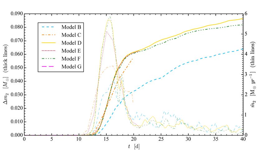
The distance a between the two particles in the orbital plane as though inconspicuous, this structure is confirmed by its presence in
a function of time is illustrated in Figure 3, solid blue for Model A other snapshots, not shown). The toroidal structure in Model B is
and dashed light blue for Model B. Jagged solid red and dashed suggestive of a thick accretion disc and is accompanied by a low-
orange lines are plotted to show the radius of the sphere within density elongated bi-polar structure, seen in blue in the bottom-right
which the resolution is at the highest refinement level, while solid panel of Figure 4. Accretion is conspicuously the cause for the pres-
green and dashed light green show the spline softening radius, for ence of this striking morphology in Model B. Below we examine
Models A and B respectively. The initial reduction in separation for the properties of the flow around the companion in more detail for
the first ∼ 12 d is known as the plunge-in phase, and each subsequent both runs.
oscillation corresponds to a full orbit of 2π radians.
The curves for Models A and B are almost identical up to
t ≈ 15 d, at which point they begin to diverge slightly. This time 3.2 ‘Accretion’ in the absence of a subgrid model (Model A)
does not correspond to any change in refinement radius or softening
For Model A, subgrid accretion is turned off, but we can measure the
length, but approximately to the time of peak in the accretion rate for
rate of mass flowing toward the secondary. We show this in the top
Model B, as will be discussed in Section 3.2. The initial differences
panel of Figure 5 by calculating and plotting the gas mass contained
after t = 14 d are thus convincingly caused by the difference in
inside spheres of a given ‘control’ radius centred on the secondary
accretion prescriptions between the two runs. In Model A, 10 orbits
versus time (RT08; RT12). The radius of the control sphere used for
are completed by t = 40 d, while in Model B, 9 orbits are completed,
the different curves is shown in the legend. The green vertical line
so the mean orbital frequency is higher in Model A between t = 15 d
indicates the time at which the softening length is halved. Times of
and t = 40 d than for Model B. This is consistent with the mean
apastron and periastron passage are marked on the horizontal axis
inter-particle separation being slightly lower for Model A than for
with long blue and short orange tick-marks, respectively. As stated
Model B during the same time interval. From t ∼ 15–17 d however,
earlier, the mass of the secondary and primary sink particles are
Model B shows a smaller separation and mean orbital period than
m2 = 0.978M , and m1 = 0.369M respectively.
Model A and vice versa after t ∼ 17 d. This suggests that the
The key result is that by the end of the simulation time, the mass
reduction in softening length at t = 16.7 d causes the orbital period
flow toward the secondary has stopped. This is in sharp contrast to
to decrease in Model A, compared to what it would have been had the
the case Model B discussed in Section 3.3.
softening length remained the same, whereas the subgrid accretion
causes a reduced orbital period in Model B between t ∼ 15–17 d,
from what it would have been had subgrid accretion been turned
3.2.1 More detailed description of time evolution
off. Therefore, both subgrid accretion and reduction of the softening
length tend to reduce the orbital period and mean separation. We The qualitative behaviour of the curves is approximately independ-
elaborate on this in Sections 3.2 and 4. ent of the control radius in that their shapes are very similar even
Both curves of separation vs. time resemble that of ORPS16. though their amplitudes differ. This tells us that the flow near the
However, in that work the particles complete only 7 orbits by t = secondary is ‘global’; different radii move inward or outward con-
40 d. Moreover, their first minimum is lower than the second, which temporaneously (on average over each spherical control surface).
is not the case in our runs, where the minima and maxima decrease The inflow rate MÛ in,2 is very small until t ≈ 10 d, increas-
monotonically with time. Furthermore, the eccentricity of the orbit, ing between t ≈ 12.5 d and t ≈ 13.5 d, peaking later for smaller
which is related to the amplitude of the separation curve, is larger control radii. During this time, Min,2 increases monotonically be-
in ORPS16. The main cause for these differences is probably that fore reaching a local maximum at t = 15 d and then decreases
in ORPS16 the RG is initialized with a solid body rotation of 95% before increasing again (this is most conspicuous for control radius
corotation, whereas in our case the initial angular rotation speed is 3R ). This local maximum coincides with the first maximum in the
zero, but it would be interesting to explore the effects of initial spin inter-particle separation curve of Figure 3. As Min,2 increases, the
in a future study. softening length is halved at t = 16.7 d. This results in a prolonged
We now turn to the insets of Figure 3, where the orbits are increase, modulated by small oscillations, until t ≈ 21 d, the time of
plotted for Model A on the left and for Model B on the right. The the third periastron passage, The average interior mass then remains
orbit of the primary particle is shaded in red/orange and the second- roughly constant, with small oscillations. The latter correspond to
ary in blue/light blue. The spline softening spheres are indicated oscillations in the inter-particle separation, with local maxima and
with green circles for t = 0 and, for Model A, also for t = 16.7 d, minima of Min,2 approximately coinciding with periastron and apas-
MNRAS 000, 000–000 (0000)Accretion in common envelope evolution 5
Figure 1. Density, in g cm−3 in a slice through the secondary and parallel to the xy (orbital) plane, for Model A (no subgrid accretion model). The secondary
is positioned at the centre with the frame rotated so that the primary particle is always situated to its left (the plotted frame of reference is rotating with the
instantaneous angular velocity of the particles’ orbit). Both particles are denoted with a green circle with radius equal to the spline softening length. Snapshots
from left to right are at t = 0, 10, 20 and 40 d.
Figure 2. As Fig. 1 but now for Model B, with the KMK04 subgrid accretion model turned on for the secondary.
tron passages respectively. The mean value of Min,2 slowly declines gas dynamical friction on the secondary (RT08; RT12; MacLeod
after t ≈ 28 d. et al. 2017). This drag may be enhanced as the quasi-steady en-
The initial rise in Min,2 is accompanied by a less pronounced velope around the secondary becomes more concentrated, thereby
rise in Min,1 until t ≈ 13 d (just after the first periastron passage), explaining the reduction in mean separation a, and, from Kepler’s
followed by a sharp decrease (not shown). Like Min,2 , Min,1 receives law, the reduction in orbital period. There is opportunity to explore
a ‘boost’ immediately following the change in softening radius at the dynamics in detail in future work.
t = 16.7 d followed by gradual decay, and modulated by oscillations Finally, the slow decrease in the secondary and primary interior
that are approximately in phase with those of Min,2 . masses Min,2 and Min,1 during the final ≈ 12 d can tentatively be
explained by the reduction in size of the Roche lobes as the inter-
These features can tentatively be explained as follows. As the
particle separation becomes smaller.
plunging-in secondary approaches the high-density RG core, it ac-
At the end of the simulation the mass flow toward the secondary
cretes at an ever higher rate, until it has accreted a quasi-steady en-
stops. The total mass ‘accreted’ by the companion Min,2 is 4 × 10⁻⁴ ,
velope. The mean mass of this envelope over several orbits remains
approximately constant. The primary retains part of the remnant 2 × 10⁻³ , 7 × 10⁻³ and 1.3 × 10⁻² M for control radii R /2, R ,
RG envelope. As the two particles approach, a larger portion of the 2R and 3R , respectively. The corresponding peak inflow rates
primary envelope extends into the control sphere surrounding the MÛ in,2 are 0.1, 0.3, 0.8 and 1.9M yr−1 , respectively. The values of
secondary, increasing the integrated mass inside the control spheres Min,2 are similar to those of Ricker & Taam (2008, 2012), though
around both particles. When the particles separate, Min,2 and Min,1 at the end of their simulation Min,2 is still increasing. However,
decrease again for the same reason. This back-and-forth motion their simulation lasted for a smaller number of orbits, so may only
explains the aforementioned oscillations. correspond to the early stages of our simulation before infall stops.
When the softening radius is reduced from rs = rs,0 to
rs = rs,0 /2, the depth of the potential well doubles at r = 0 and
3.3 ‘Accretion’ with a subgrid model (Model B)
the gravitational acceleration of each particle increases everywhere
within the sphere of the original softening radius rs,0 centred on We now turn to Model B, which includes KMK04 subgrid accretion.
the particle. Gas then flows toward the secondary until a more The key results are shown in the bottom panel of Figure 5.
massive, more concentrated quasi-steady envelope establishes. A The pressure release valve provided by the Krumholz subgrid
weaker similar effect occurs for the less massive primary particle. model in Model B allows mass to flow continuously onto the sec-
The gradual decrease in the orbital separation is likely caused by ondary without stopping, unlike Model A, for which the mass inflow
MNRAS 000, 000–000 (0000)6 L. Chamandy et al.
Figure 3. Inter-particle separation in the orbital plane (z = 0) for Model A, without subgrid accretion (solid blue), and Model B, with subgrid accretion (dashed
light blue). Also shown are jagged lines denoting the radius of the spherical region of highest mesh refinement (solid red for Model A and dashed orange for
Model B), and the spline softening radius (solid green for Model A and dashed light green for Model B). Inset: Orbit of the sink-particles, with Model A
depicted on the left and Model B on the right. The centre of mass is located at the origin in each panel. The primary particle is shown in red/orange while
the secondary is shown in blue/light blue. Green/light green circles with radius equal to the spline softening length are shown at t = 0 and, for Model A, also
at t = 16.7 d, when the softening length is halved. (The sampling rate used to draw the orbits is about one frame per 0.23 d, resulting in a slightly “choppy”
appearance at late times that is not related to the time sampling in the simulation.)
stops and the envelope mass around the secondary remains quasi- 3.4 Velocity field around the secondary
steady. The actual (subgrid) accretion rate onto the secondary is
Exploring the flow properties around the secondary helps to assess
shown in the bottom panel of Figure 5, where we plot the evolu-
the plausibility of disc formation at even smaller, unresolved dis-
tion of the change in secondary mass ∆m2 , along with the rate of
tances from the secondary (< rs ). In Figure 6 we plot in color the
change mÛ 2 .5 Accretion begins at t ≈ 12 d, coinciding with the first
local tangential velocity vφ,2 with respect to the secondary in the
periastron passage. The accretion rate mÛ 2 peaks between t = 16 d
frame of reference that rotates at the instantaneous angular velocity
and t = 17 d at mÛ 2 ≈ 2.7M yr−1 . By the end of the simulation, the
of the particle orbit about the secondary. Shown is a slice through the
accretion rate reaches a fairly steady value of mÛ 2 ≈ 0.3M yr−1 ,
secondary perpendicular to the z-axis at t = 40 d, with green circles
modulated by oscillations likely related to the oscillations in the
demarking the spline softening spheres. Here vφ,2 is normalized
inter-particle separation. By the end of the simulation at t = 40 d
with respect to the Keplerian speed vK about the secondary, cor-
the secondary has accreted 0.064M , for a 6.5% gain in mass, and
rected for the spline potential within the softening radius. A white
continues to accrete.
contour delineates where vφ,2 = 0, and the vectors show the direc-
The plots of Min,2 and Min,1 and their rates of change for
tion and relative magnitude of the velocity field of the gas projected
Model B (not shown) are qualitatively similar to those for Model A,
onto the slice.
but the fractional decrease in Min,2 between its peak and t = 40 d is
Figure 6 shows that vφ,2 > 0 within about 3 to 4R of the
≈ 5 times greater in Model B than in Model A, while the fractional
secondary for Model A, and within about 5 to 6R of the secondary
decrease in Min,1 from the time that Min,2 peaks to t = 40 d is only
for Model B. Outside of this region, the gas rotates clockwise (vφ,2 <
≈ 20 per cent greater. Since the main difference between Model A
0), lagging the orbital motion of the particles in the lab frame. Inside
and Model B is the presence or absence of subgrid accretion, this
the region of counter-clockwise rotation, the vectors show that the
result is consistent with the finding that the gas flow around the
gas exhibits both positive and negative radial velocity vr,2 . The
secondary is influenced by the subgrid accretion in Model B.6
magnitude of the tangential component is ∼ 51 VK to ∼ 14 VK within
5 The rate is calculated using a central difference method accurate to second
order. The sampling rate is constant and approximately equal to one frame
every 0.23 d. Model B and the fact that in Model B, Min,2 peaks at t ≈ 17 d, much earlier
6 However, the reduction in softening length applied in Model A but not in than in Model A, may also play a role.
MNRAS 000, 000–000 (0000)Accretion in common envelope evolution 7
Figure 4. Gas density in g cm−3 viewed in a slice through both particles that is perpendicular to the orbital plane at t = 40 d. Model A (no subgrid accretion) is
shown in the left-hand column and Model B (KMK04 subgrid accretion) is shown in the right-hand column, while the top and bottom row show two different
levels of zoom (with different color schemes to aid viewing). The secondary is situated in the centre of each panel and the frame is rotated so that the primary
particle is located to its left. Spline softening spheres are identified by green circles. The x 0 -axis is defined by the line in the orbital plane that passes through
both sink particles.
about 2R from the softening radius in both simulations. We discuss to form, we can simply assume conservation of specific angular mo-
the implications of this angular motion in the next section. mentum of the flow around the secondary at r & rs and determine if
the flow would be purely rotationally supported at r & R∗ . Assum-
ing that any net angular momentum transport would be outward, this
condition sets an upper limit on the stellar radius that would still
4 IMPLICATIONS FOR ACCRETION IN CEE leave room for a Keplerian thin disc to form. The specific angular
momentum at radius r = r√s (averaged over√azimuth, in the orbital
4.1 Condition for accretion disc formation
plane) can be written as f Gm2 rs , where Gm2 r is the Keplerian
The sub-Keplerian speeds of the gas flowing around the secondary value at radius r and f 6 1 is a parameter that can be estimated
imply that a relatively thick disc forms on resolved scales, although from the simulations. The upper limit to the stellar radius for disc
this does not by itself determine the disc structure within r < rs formation is then given by
from the secondary, where gravity is not treated fully realistically in
R∗ . f 2 rs . (1)
our model (see also the next subsection). This point is particularly
germane when the secondary is a WD with radius R∗ ∼ 0.01R – Section 3.4 shows that 1/5 . f . 1/4 for both Model A
far smaller than the softening radius and comparable to the size of (rs (40 d) = 1.2R ) and Model B (rs = 2.4R ). This translates
the smallest resolution element. into a maximum stellar radius of 0.05R . R∗,max . 0.08R for
To assess the minimum condition needed for an inner thin disc Model A and 0.10R . R∗,max . 0.15R for Model B. This result
MNRAS 000, 000–000 (0000)8 L. Chamandy et al.
Figure 5. Top panel: ‘Accretion’ by the companion for Model A, which is not true accretion because no subgrid accretion model is used. The total mass
contained within spheres of various radii is shown in blue, with line styles corresponding to control radii (see legend). A vertical green line marks the time at
which the softening length is reduced by half. Bottom panel: Accretion by the companion for Model B, for which the KMK04 subgrid accretion model is used.
The accreted mass is shown in blue (left-hand vertical axis) and the accretion rate, obtained by differentiating the accreted mass, is shown in red (right-hand
vertical axis). For both panels, long light blue (short orange) tick marks show the times of apastron (periastron) passage, seen in Figure 3. (Where the sampling
rate for the inter-particle separation was lower, times of apastron/periastron passage were obtained after performing an interpolation.)
MNRAS 000, 000–000 (0000)Accretion in common envelope evolution 9
Figure 6. Slice through the orbital plane at t = 40 d with colour showing the tangential (with respect to the secondary, located at the centre of each panel)
component of the velocity in the frame of reference rotating about the secondary with the instantaneous orbital angular velocity of the sink particles. Values
are normalized by the local Keplerian circular speed around the secondary, corrected for the spline potential inside the softening sphere. The zero value, where
the tangential component reverses direction, is shown by a white contour. Vectors show the direction and magnitude of the projection of this same velocity
onto the orbital plane (each vector refers to the location at which its tail begins). Model A (no subgrid accretion) is shown on the left and Model B (KMK04
subgrid accretion) is shown on the right. Softening spheres are indicated by green circles.
suggests that a purely Keplerian thin accretion disc would not be 4.3 Super-Eddington Accretion
able to form if the star is a MS star (R∗ ∼ 1R ), but that there is
As material accretes from the envelope to the secondary, we estimate
still plenty of room for a thin accretion disc to form if the secondary
from the virial theorem that about half of the liberated potential
is a WD (R∗ ∼ 0.01R ). Disc thinness is not a necessary property
energy will ultimately be added to the accretor in the form of thermal
for dynamically significant accretion and a jet. Super-Eddington
energy. The remainder will be transferred to the optically thick
accretion could produce a radiation-dominated thick disc which
envelope in the form of bulk kinetic and thermal energy. The rate
facilitates collimated radiation-driven outflows. However, for jets
of this energy transfer can be estimated as
that depend on Poynting flux anchored in the disc, the outflow
power is proportional to the angular velocity at the field anchor Gm2 mÛ 2
EÛacc = , (2)
point so too slow a rotator would reduce the outflow power. All of 2λR
e ∗
this warrants further work.
where R∗ is the radius of the accretor, and λ e is a parameter of
order unity that depends on the density profile of the accretor and is
analogous to the parameter λ often invoked for the primary envelope
in CE calculations (Ivanova et al. 2013, and references therein). For
this formula, we assumed that 1/R∗
1/ri , where ri is the initial
radius of the accreting gas with respect to the centre of the accretor.
We have also neglected the change in potential energy associated
4.2 Need for a pressure valve with the primary particle and with the self-gravity of gas.
Comparing the no-accretion case with the KMK04 case highlights Assuming an opacity due to electron scattering, the Eddington
that sustained long term accretion requires a pressure valve. The accretion rate onto the secondary is given by
KMK04 prescription takes away both mass and pressure, allowing 4πmp Gm2
material to continue to infall at the inner boundary. If we disallow mÛ 2, Edd = , (3)
cσT
this infall, the accretion flow eventually ceases. The KMK04 pre-
where mp is the proton mass, c is the speed of light in vacuum, σT is
scription was originally developed for protostellar accretion where
the Thomson scattering cross section, and σT /mp = 0.398 cm2 g−1 .
material that accretes onto the central object can lose its pressure
The radiative efficiency is the fraction of the rest-mass energy of
via radiation through optically thin gas. In the present case, the gas
accreted material that is transferred to the envelope. Thus we write
is optically thick, so we do not expect such pressure to release ra-
diation. Jets (Staff et al. 2016; Moreno Méndez et al. 2017; Soker EÛacc
= , (4)
2017) provide a more likely alternative. In fact, we suspect that mÛ 2 c2
jets may provide the only way to sustain accretion in these dense
where EÛacc is the rate of energy transferred to the envelope due to
environments, implying a mutually symbiotic relation and one-to-
accretion. Substituting expression (2) into equation (4) and then the
one correspondence between the two. Since a jet would provide a
resulting expression for into equation (3), we obtain an efficiency
pressure release valve that is not as large as that of the KMK04
prescription, our two cases (no accretion vs. accretion) bound the R∗ −1
= 1.1 × 10⁻⁶ λ e−1 m2 (5)
extreme cases of maximum and zero valve. M R
MNRAS 000, 000–000 (0000)10 L. Chamandy et al.
and an Eddington accretion rate et al. 2018), particularly within the softening length (ORPS16). The
resolution can affect the orbit and fidelity of energy conservation in
e R∗ .
mÛ 2, Edd = 2.1 × 10⁻³ M yr−1 λ (6) the final phases of inspiral. Second, the softening length itself must
R be sufficiently small, for the reasons discussed above. But making
This is not a strict upper limit because it assumes energy release rs comparable to the stellar radius is also problematic because,
as radiation and spherical symmetry, so can be circumvented to as we have emphasized, the choice of subgrid model for physics
some extent if the energy is transported by a bipolar jet. From the near the stellar surface (e.g. accretion, jets, convection) becomes
bottom panel of Figure 5, we see that accretion rates of order 0.2 influential. Third, the spatial extent of the region surrounding the
to 2 M yr−1 are obtained for our ∼ 1M secondary. For a MS star particles within which the resolution is highest must be large enough
with radius 1 R , this translates to accretion rates 102 to 103 times to prevent inaccuracies in the particles’ orbit for instance. This can
larger than the Eddington rate, while for a WD with radius 0.01 R , arise due to the particles’ non-circular orbit and the complex nature
we find that mÛ 2 is 104 to 105 times the Eddington rate. of the flow: particles can end up interacting strongly with gas that
had not been well-resolved at some earlier time.
Other choices about the numerical setup must be made, like the
4.4 Implications for CE PNe and PPNe size of the domain and base resolution, but the three considerations
The possibility of so-called super-Eddington or hypercritical accre- listed above are most crucial for studying CEE near the particles.
tion and its potential role in unbinding the CE is discussed in Ivanova In this work, we chose values for the size of the smallest res-
et al. (2013); Shiber et al. (2016). Although steady accretion onto a olution element (0.07 to 0.14R ), softening length (1.2 to 2.4R ),
WD or MS star at such extreme rates would likely be substantially and refinement radius (see Figure 3) that are ‘conservative’ to en-
mitigated by feedback from the accretion processes closer to the sure qualitatively physical results. However, a convergence study
stellar surface, super-Eddington values may be possible. that explores each of these parameters separately while keeping the
As discussed in the introduction jets produced by accretion also other two fixed, is warranted. But given the extensive computational
play an important role in shaping PPNe and PNe. Depending on the resources required, we leave such a comprehensive study for future
engine (WD or MS star), momentum requirements for a number of work.
PPNe would seem to require accretion rates close to this limit and Preliminary tests at lower resolution do suggest that each of
would have to be achieved either within the CE or the Roche-lobe the three constraints can be important, and we present an analysis of
overflow phase just before Blackman & Lucchini (2014). Were it the a limited set of test runs in Appendix A. Depending on the goals of
case that a jet could not form or sustain inside the CE because the a particular investigation, a convergence study can help determine
pressure valve were simply not efficient enough, we would be led which one or more of the three parameter values can be relaxed
to conclude that evidence for accretion-powered outflows in PPNe (i.e. our choices could be adjusted to be more ‘aggressive’), and in
could not emanate from inside the CE but more likely from the turn, help optimize the use of computational resources.
Roche Lobe overflow phase (Staff et al. 2016) before CE. There is
much opportunity for future work to study the fate of a jet formed
outside the CE as it enters the CE. 6 CONCLUSIONS
We have presented a new platform for simulating CEE. Our As-
troBEAR AMR MHD multi-physics code (Cunningham et al. 2009;
5 NUMERICAL CHALLENGES AND NEED FOR
Carroll-Nellenback et al. 2012) has been adapted to model the in-
CONVERGENCE STUDY
teraction of an extended giant star with a companion modeled as a
In Section 3 we explained how the particles’ orbits and the flow point mass. We have used the platform to carry out two high resol-
around the secondary are affected when the spline softening length ution simulations of CE interaction with the goal of assessing the
rs is halved in Model A from 2.4R to 1.2R at t = 16.7 d. We nature of accretion onto the secondary. Our Model B employed a
argued that this change leads to a reduced orbital period and separa- subgrid model for accretion that removes mass and pressure from the
tion, and to a denser envelope of material around the secondary than grid, effectively making the secondary a point mass “sink” particle
what would have obtained had rs been kept constant as in Model B. (KMK04). No subgrid model was employed in our Model A sim-
Such behaviour is unphysical because the gravitational softening is ulation and so gravitationally bound material that collected around
a numerical device that is imposed to deal with finite resolution. the secondary was not removed from the grid.
In reality, there would be a stellar surface, at r ∼ 1R for a MS For both simulations, AstroBEAR accurately models the main
secondary or at r ∼ 0.01R for a WD secondary. For the latter, features of CEE when compared to previous simulations. In partic-
any imposed softening length should ideally be
1R , and yet the ular, the code captures the rapid inspiral of the secondary as well as
softening length must be adequately resolved, e.g. to ensure energy the conservation of orbital energy into mass motions of the envelope
conservation (ORPS16). which can unbind a fraction of the gas
In Model A we followed ORPS16 by requiring that rs not With regard to our main focus question of accretion onto the
exceed 1/5 of the inter-particle separation. That this changes the secondary, we find that only for Model B, where a subgrid model
orbit and flow suddenly, when the softening length is halved just is used to remove mass and pressure near the secondary particle,
before the threshold 1/5 is reached, implies that 1/5 is too large. does gas continue to accrete onto the secondary core. In con-
This suggests that finite softening lengths produce overestimates of trast, for Model A, mass collects around the secondary, forming
the inter-particle separations at late times in global CE simulations. a quasi-stationary extended high pressure atmosphere whose accre-
This is consistent with a conclusion of Iaconi et al. (2018), that final tion eventually shuts off. This is important because accretion and
separations decrease with decreasing smoothing length. accretion discs are tied to the generation of outflows/jets. Such out-
What makes CE simulations computationally demanding is flows from deep in a stellar interior have been considered as the
the need to simultaneously satisfy three crucial constraints. First is means for driving some classes of supernova (Milosavljević et al.
that the resolution near the particles should be high enough (Iaconi 2012; Gilkis et al. 2016). As Sabach & Soker (2015); Soker (2015);
MNRAS 000, 000–000 (0000)Accretion in common envelope evolution 11
Shiber et al. (2017); Shiber & Soker (2018) have shown in their Carroll-Nellenback J. J., Shroyer B., Frank A., Ding C., 2013, Journal of
“Grazing Envelope” models, the presence of strong jets can lead Computational Physics, 236, 461
to the envelope material being driven out of the CE system. We Cunningham A. J., Frank A., Varnière P., Mitran S., Jones T. W., 2009,
have shown that accretion onto the secondary in CEE can produce ApJS, 182, 519
super-Eddington accretion rates on either a MS star or WD but only De Marco O., Izzard R. G., 2017, PASA, 34, e001
Edgar R., 2004, New Astron. Rev., 48, 843
if there is a “pressure release valve” for maintaining steady flows
Eggleton P. P., 1983, ApJ, 268, 368
during the inspiral. Since the CE environments are optically thick Frank J., King A., Raine D. J., 2002, Accretion Power in Astrophysics: Third
we are led to speculate that jets may be the only way to sustain Edition
accretion. As such, there would be a one-to-one correspondence Gilkis A., Soker N., Papish O., 2016, ApJ, 826, 178
between active accretion and jets in CEE. Glanz H., Perets H. B., 2018, preprint, (arXiv:1801.08130)
If bipolar outflows can be sustained in CEE, they are candidates Grichener A., Sabach E., Soker N., 2018, preprint, (arXiv:1803.05864)
to supply the outflow momentum and energy budgets needed to Hoyle F., Lyttleton R. A., 1939, Proceedings of the Cambridge Philosophical
explain PPN bipolar jets. Otherwise, accretion-powered jets could Society, 35, 405
still be produced in the Roche lobe phase just before entering the Iaconi R., Reichardt T., Staff J., De Marco O., Passy J.-C., Price D., Wurster
CE. J., Herwig F., 2017, MNRAS, 464, 4028
Iaconi R., De Marco O., Passy J.-C., Staff J., 2018, MNRAS,
Finally, as was noted in the introduction, the ejection of the en-
Iben Jr. I., Livio M., 1993, PASP, 105, 1373
velope and the completion of the inspiral to small radii has proven
Ivanova N., Nandez J. L. A., 2016, MNRAS, 462, 362
difficult to achieve in simulations (Ohlmann et al. 2016; Kuruwita Ivanova N., et al., 2013, ARA&A, 21, 59
et al. 2016) including ours without additional feedback. Explana- Jones D., Boffin H. M. J., 2017, Nature Astronomy, 1, 0117
tions for this behaviour split between those focusing on limits of the Kalogera V., Belczynski K., Kim C., O’Shaughnessy R., Willems B., 2007,
numerics and those that focus on limits in the physics. For numerics PhR, 442, 75
the concern relates to resolution and timescales. For physics the Krumholz M. R., McKee C. F., Klein R. I., 2004, ApJ, 611, 399
concern is that there are important physical processes not included Kuruwita R. L., Staff J., De Marco O., 2016, MNRAS, 461, 486
in the numerical models. Examples of such processes include re- Li S., Frank A., Blackman E. G., 2014, MNRAS, 444, 2884
combination and radiation pressure on dust. While recombination Livio M., Soker N., 1988, ApJ, 329, 764
has received positive attention, newer work casts some doubt on its Lombardi Jr. J. C., Proulx Z. F., Dooley K. L., Theriault E. M., Ivanova N.,
Rasio F. A., 2006, ApJ, 640, 441
efficacy (Soker & Harpaz 2003; Sabach et al. 2017; Grichener et al.
MacLeod M., Ramirez-Ruiz E., 2015a, ApJ, 798, L19
2018). There is much opportunity to further delineate the role of
MacLeod M., Ramirez-Ruiz E., 2015b, ApJ, 803, 41
accretion and outflows in CEE alongside the other envelope loss MacLeod M., Antoni A., Murguia-Berthier A., Macias P., Ramirez-Ruiz E.,
physics mechanisms, and the mutual connection if any, to further 2017, ApJ, 838, 56
orbital decay. MacLeod M., Ostriker E. C., Stone J. M., 2018, preprint,
(arXiv:1803.03261)
Milosavljević M., Lindner C. C., Shen R., Kumar P., 2012, ApJ, 744, 103
Moreno Méndez E., López-Cámara D., De Colle F., 2017, MNRAS, 470,
ACKNOWLEDGEMENTS
2929
LC wishes to thank Sebastian Ohlmann for helpful discussions Murguia-Berthier A., MacLeod M., Ramirez-Ruiz E., Antoni A., Macias P.,
relating to methods. The authors gratefully acknowledge Or- 2017, ApJ, 845, 173
Nandez J. L. A., Ivanova N., Lombardi Jr. J. C., 2014, ApJ, 786, 39
sola De Marco, Paul Ricker, Morgan MacLeod, Brian Metzger,
Nandez J. L. A., Ivanova N., Lombardi J. C., 2015, MNRAS, 450, L39
Natalia Ivanova, Noam Soker and Hui Li for thought-provoking
Nelemans G., Verbunt F., Yungelson L. R., Portegies Zwart S. F., 2000,
conversations during the time this work was being prepared. JN A&A, 360, 1011
acknowledges financial support from NASA grants HST-15044 and Nordhaus J., Blackman E. G., 2006, MNRAS, 370, 2004
HST-14563. Nordhaus J., Blackman E. G., Frank A., 2007, MNRAS, 376, 599
Nordhaus J., Wellons S., Spiegel D. S., Metzger B. D., Blackman E. G.,
2011, Proceedings of the National Academy of Science, 108, 3135
Ohlmann S. T., Röpke F. K., Pakmor R., Springel V., 2016, ApJ, 816, L9
Ohlmann S. T., Röpke F. K., Pakmor R., Springel V., 2017, A&A, 599, A5
References
Paczynski B., 1976, in Eggleton P., Mitton S., Whelan J., eds, IAU Sym-
Abbott B. P., et al., 2016, Physical Review Letters, 116, 061102 posium Vol. 73, Structure and Evolution of Close Binary Systems. p. 75
Abbott B. P., et al., 2017a, Physical Review Letters, 119, 141101 Passy J.-C., et al., 2012, ApJ, 744, 52
Abbott B. P., et al., 2017b, Physical Review Letters, 119, 161101 Paxton B., Bildsten L., Dotter A., Herwig F., Lesaffre P., Timmes F., 2011,
Balick B., Frank A., 2002, ARA&A, 40, 439 ApJS, 192, 3
Belczynski K., Buonanno A., Cantiello M., Fryer C. L., Holz D. E., Mandel Paxton B., et al., 2013, ApJS, 208, 4
I., Miller M. C., Walczak M., 2014, ApJ, 789, 120 Paxton B., et al., 2015, ApJS, 220, 15
Blackman E. G., Lucchini S., 2014, MNRAS, 440, L16 Rasio F. A., Livio M., 1996, ApJ, 471, 366
Blackman E. G., Frank A., Welch C., 2001, ApJ, 546, 288 Reyes-Ruiz M., López J. A., 1999, ApJ, 524, 952
Blank M., Morris M. R., Frank A., Carroll-Nellenback J. J., Duschl W. J., Ricker P. M., Taam R. E., 2008, ApJ, 672, L41
2016, MNRAS, 459, 1721 Ricker P. M., Taam R. E., 2012, ApJ, 746, 74
Bondi H., 1952, MNRAS, 112, 195 Sabach E., Soker N., 2015, MNRAS, 450, 1716
Bondi H., Hoyle F., 1944, MNRAS, 104, 273 Sabach E., Hillel S., Schreier R., Soker N., 2017, MNRAS, 472, 4361
Bujarrabal V., Castro-Carrizo A., Alcolea J., Sánchez Contreras C., 2001, Sahai R., Vlemmings W. H. T., Gledhill T., Sánchez Contreras C., Lagadec
A&A, 377, 868 E., Nyman L.-Å., Quintana-Lacaci G., 2017, ApJ, 835, L13
Carroll-Nellenback J., Shroyer B., Frank A., Ding C., 2012, in Pogorelov Sandquist E. L., Taam R. E., Chen X., Bodenheimer P., Burkert A., 1998,
N. V., Font J. A., Audit E., Zank G. P., eds, Astronomical Society of ApJ, 500, 909
the Pacific Conference Series Vol. 459, Numerical Modeling of Space Sandquist E. L., Taam R. E., Burkert A., 2000, ApJ, 533, 984
Plasma Slows (ASTRONUM 2011). p. 291 (arXiv:1112.1710) Shiber S., Soker N., 2018, MNRAS,
MNRAS 000, 000–000 (0000)You can also read