Comparison of uncertainties in land-use change fluxes from bookkeeping model parameterisation
←
→
Page content transcription
If your browser does not render page correctly, please read the page content below
Earth Syst. Dynam., 12, 745–762, 2021
https://doi.org/10.5194/esd-12-745-2021
© Author(s) 2021. This work is distributed under
the Creative Commons Attribution 4.0 License.

               Comparison of uncertainties in land-use change
               fluxes from bookkeeping model parameterisation
       Ana Bastos1,2 , Kerstin Hartung1,a , Tobias B. Nützel1 , Julia E. M. S. Nabel3 , Richard A. Houghton4 , and
                                                    Julia Pongratz1,3
               1 Department  of Geography, Ludwig Maximilian University of Munich, 80333 Munich, Germany
       2 Max   Planck Institute for Biogeochemistry, Department of Biogeochemical Integration, 07745 Jena, Germany
                               3 Max Planck Institute for Meteorology, 20146 Hamburg, Germany
                               4 Woodwell Climate Research Center, Falmouth, MA 02540, USA
                  a now at: Deutsches Zentrum für Luft- und Raumfahrt, Institut für Physik der Atmosphäre,

                                                  Oberpfaffenhofen, Germany
                                  Correspondence: Ana Bastos (abastos@bgc-jena.mpg.de)

                                 Received: 13 December 2020 – Discussion started: 11 January 2021
                              Revised: 11 June 2021 – Accepted: 19 June 2021 – Published: 30 June 2021

       Abstract. Fluxes from deforestation, changes in land cover, land use and management practices (FLUC for
       simplicity) contributed to approximately 14 % of anthropogenic CO2 emissions in 2009–2018. Estimating FLUC
       accurately in space and in time remains, however, challenging, due to multiple sources of uncertainty in the
       calculation of these fluxes. This uncertainty, in turn, is propagated to global and regional carbon budget estimates,
       hindering the compilation of a consistent carbon budget and preventing us from constraining other terms, such as
       the natural land sink. Uncertainties in FLUC estimates arise from many different sources, including differences in
       model structure (e.g. process based vs. bookkeeping) and model parameterisation. Quantifying the uncertainties
       from each source requires controlled simulations to separate their effects.
          Here, we analyse differences between the two bookkeeping models used regularly in the global carbon
       budget estimates since 2017: the model by Hansis et al. (2015) (BLUE) and that by Houghton and Nas-
       sikas (2017) (HN2017). The two models have a very similar structure and philosophy, but differ significantly
       both with respect to FLUC intensity and spatiotemporal variability. This is due to differences in the land-use
       forcing but also in the model parameterisation.
          We find that the larger emissions in BLUE compared to HN2017 are largely due to differences in C densities
       between natural and managed vegetation or primary and secondary vegetation, and higher allocation of cleared
       and harvested material to fast turnover pools in BLUE than in HN2017. Besides parameterisation and the use of
       different forcing, other model assumptions cause differences: in particular that BLUE represents gross transitions
       which leads to overall higher carbon losses that are also more quickly realised than HN2017.

1   Introduction                                                    and management (FLUC ) result from changes in vegetation
                                                                    and soil carbon stocks and product pools due to human activ-
                                                                    ities, such as deforestation, forest degradation, afforestation
Changes in land use and management are estimated to have            and reforestation, as well as management practices such as
contributed to a global source of CO2 to the atmosphere             wood harvest and shifting cultivation (rotation cycle between
from the pre-industrial period until the present, and to ac-        forest and agriculture), and subsequent regrowth of natural
count for more than 10 % of the total CO2 emissions over            vegetation following harvest or agricultural abandonment.
the past decade according to the Global Carbon Budget 2019
(Friedlingstein et al., 2019). Fluxes from land-use change

Published by Copernicus Publications on behalf of the European Geosciences Union.
746   A. Bastos et al.: Comparison of uncertainties in land-use change fluxes from bookkeeping model parameterisation

    Reconstructing these changes consistently over the globe       in the 1950s, which is likely attributable to the change in
for the past centuries (let alone millennia) is, however, chal-    methodology in HYDE (Klein Goldewijk et al., 2017) from
lenging and associated with high uncertainties (Hurtt et al.,      using FAOSTAT (FAOSTAT, 2015) estimates to population-
2020; Klein Goldewijk et al., 2017; Pongratz et al., 2014;         based extrapolation in the past (Bastos et al., 2016). This
Ramankutty and Foley, 1999). This uncertainty in forcing           comes on top of a generally steeper increase in FLUC in
translates directly to uncertainties in FLUC estimates (Gasser     BLUE in 1870–1950. A second notable difference in tem-
et al., 2020; Pongratz et al., 2009; Stocker et al., 2011).        poral dynamics can be observed in the 2000s, as has been
Moreover, differences in definitions and terminology, and on       shown by Bastos et al. (2020). Here, BLUE shows a strong
how indirect environmental effects such as increasing atmo-        increasing trend starting 2000, while HN2017 estimates start
spheric CO2 concentration are considered lead to large dif-        decreasing after the late 1990s.
ferences in FLUC estimated by different methods (Gasser and           The estimated uncertainty of FLUC in the global carbon
Ciais, 2013; Grassi et al., 2018; Pongratz et al., 2014; Stocker   budgets is thus approximately 0.7 PgC yr−1 or approximately
and Joos, 2015). Grassi et al. (2018) have shown that by har-      ±50 % of the average value, substantially larger than that of
monising definitions of managed land, estimates of FLUC by         fossil fuel emissions. This uncertainty, in turn, is propagated
a bookkeeping (BK) model, dynamic global vegetation mod-           to global and regional carbon budget estimates and affects
els (DGVMs) and national inventories can be in part recon-         the land sink term, which has often been quantified as resid-
ciled. The indirect environmental effects (accounted for in        ual depending on FLUC . Houghton (2020) further noted that
DGVMs but not in BK models) can be calculated by fac-              while net FLUC can be constrained by the global carbon bud-
torial simulations, in order to compare estimates from these       gets, the component gross fluxes (sources such as deforesta-
two methods (Bastos et al., 2020). Whether and how these           tion and sinks, e.g. by afforestation) are even more uncertain.
indirect effects are accounted for in FLUC creates large dif-         Differences in initial land-cover distribution and transi-
ferences between estimates but can be resolved by a consis-        tions across different forcing datasets can also lead to sub-
tent terminology (Grassi et al., 2018; Pongratz et al., 2014).     stantial differences in estimated FLUC (Di Vittorio et al.,
Besides uncertainty in historical land-use change (LUC) ar-        2020; Li et al., 2018; Gasser et al., 2020). A detailed analy-
eas and terminological issues, studies also differ with respect    sis of the impact of the forcing datasets on LUC estimated by
to which LUC practices are considered. Several studies have        the OSCAR bookkeeping (BK) model has been performed by
shown that including management practices such as shifting         Gasser et al. (2020), and Hartung et al. (2021) analysed the
cultivation, crop or wood harvesting might increase FLUC by        effect of the different LUC from the Land-Use Harmoniza-
70 % or more in individual DGVM estimates (Arneth et al.,          tion dataset (LUH2v2.1) (Hurtt et al., 2020) and of various
2017; Pugh et al., 2015) with management processes explain-        internal model assumptions in BLUE on FLUC .
ing some of the differences between biospheric fluxes from            Despite the relevance of the BLUE and HN2017 estimates
DGVMs and top-down estimates (Bastos et al., 2020).                for the global carbon budget analyses, stark discrepancies
    In the global carbon budgets since 2017 (Friedlingstein        between these two models (Friedlingstein et al., 2019) and
et al., 2019; Le Quéré et al., 2018a, b), FLUC estimates           the long-standing appreciation of various factors contribut-
for recent decades are taken as the mean of the estimates          ing to such differences (Hansis et al., 2015; Houghton et al.,
of two BK models, the one from Houghton and Nas-                   2012), no quantitative analysis on the contribution of model
sikas (2017) (HN2017) and the BLUE model described                 differences to this discrepancy has so far been performed.
in Hansis et al. (2015). However, even for these similar           Both models rely on observation-based estimates for their
methods, estimates differ considerably (Bastos et al., 2020;       parameterisations and forcing datasets, and the choices on
Friedlingstein et al., 2019). Cumulative FLUC from 1850 un-        spatial and plant functional type representation, starting year
til the present day by these two BK models is 205±60 PgC in        and other aspects are well justified in both models. However,
the Global Carbon Budget 2019 (Friedlingstein et al., 2019;        these multiple differences add to uncertainty in FLUC esti-
GCB2019 in the following). The FLUC uncertainty after 1959         mates and make it difficult to attribute differences in FLUC
has been defined by best value judgement that there is a 68 %      and their trends to specific aspects of the FLUC calculation.
likelihood that actual FLUC lies within ±0.7 PgC yr−1 of the          In this study, we fill this gap and assess to which extent
two models’ mean, and for earlier periods, the standard devi-      the different parameterisations in BLUE and HN2017 affect
ation of a group of DGVMs was used. This uncertainty range         global and regional FLUC estimates and their trends. We fur-
reflects uncertainties in parameterisations of the BK models,      ther investigate the effect of the different parameter choices
in the applied land-use change forcings as well as definitions,    on the gross LUC fluxes.
processes considered, and is large enough to encompass the
two models’ estimates.
    Besides differences in cumulative FLUC , BLUE and
HN2017 also show very different temporal behaviours
(Friedlingstein et al., 2019, and see Fig. 2 below). Notewor-
thy is an increase in FLUC in BLUE but decrease in HN2017

Earth Syst. Dynam., 12, 745–762, 2021                                                https://doi.org/10.5194/esd-12-745-2021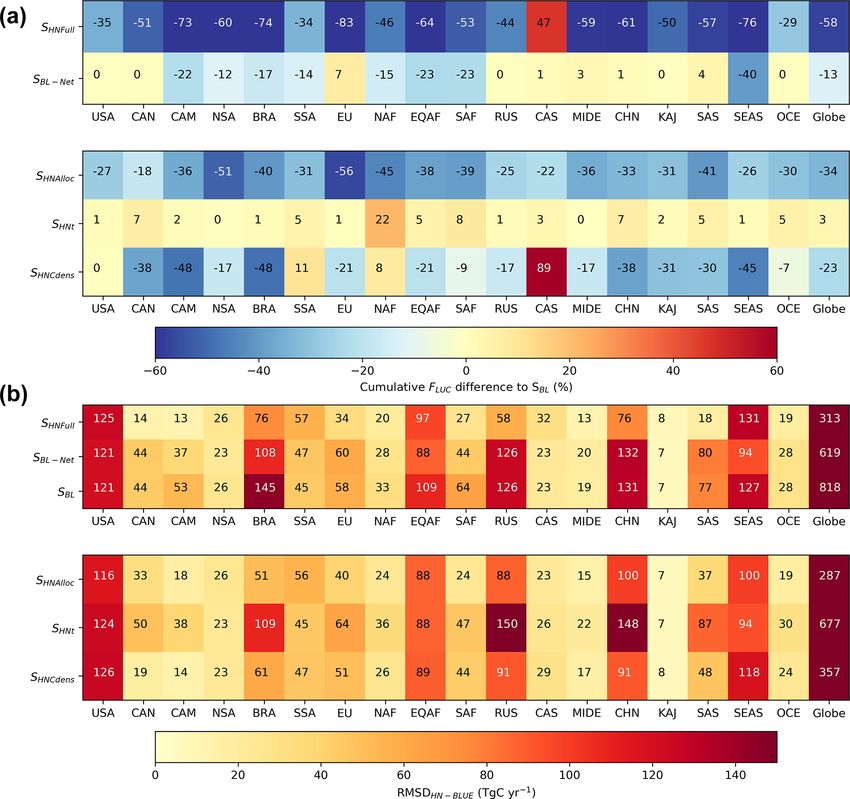
A. Bastos et al.: Comparison of uncertainties in land-use change fluxes from bookkeeping model parameterisation              747

2     Data and methods                                             sity in above- and below-ground pools which are plant func-
                                                                   tional type (PFT) specific and based on measurements (Ta-
2.1    Model characteristics and datasets used                     ble A2). However, the models differ in the number of plant
                                                                   functional types (Table A1) and their spatial distribution (per
In this study, we focus on the two BK models used in the           country in HN2017 and spatially explicit in BLUE).
GBC2019 as well as in the Intergovernmental Panel on Cli-             For harvest and clearing, the dislocated C is distributed
mate Change’s Special Report on Climate Change and Land            between a dead soil pool and three product pools of differ-
(IPCC, 2019) to estimate FLUC : the Bookkeeping of Land-           ent lifetimes: 1, 10 and 100 years (Table A3). In the case
Use change Emissions model, BLUE (Hansis et al., 2015)             of BLUE these fractions are fixed and PFT specific, while
and the model from Houghton and Nassikas (2017), which is          HN2017 distinguishes between harvested wood use over
referred to as HN2017.                                             time (fuel, 1-year, industrial, 10- and 100-year timescales),
   The two models differ in several aspects, the most rele-        so that the fraction allocated to each pool changes over time.
vant ones summarised in Table 1. An important difference,             Parameters in BLUE and HN2017 are defined on a PFT
which we will account for in this study, is that BLUE esti-        basis, but HN2017 distinguishes 20 PFTs (3 of them desert
mates FLUC from gross LUC transitions, while HN2017 uses           PFTs), while BLUE distinguishes 11 PFTs. In order to com-
net transitions. Gross transitions resolve that within a unit      pare the parameterisations, the different PFTs need to be
(grid cell for BLUE, country/region for HN2017) there may          mapped. Most HN2017 PFTs can be aggregated into the of-
be concurrent back-and-forth transitions between a pair of         ten more broadly defined BLUE PFTs but some of the PFTs
land-use types; for example, 30 % of the unit area may be          in BLUE do not correspond to HN2017 PFTs (e.g. sum-
transformed from forest to cropland, while on 20 % cropland        mergreen shrubs) (Table A1). A map of the PFT distribu-
is abandoned and forest regrows. Net transitions would rep-        tion from HN2017 is not available, as the PFT fractions are
resent this as a 10 % forest to cropland transition. These sub-    defined on a per-country basis. When aggregated globally,
unit changes are particularly important for large units (large     the values of BLUE and HN2017 show good agreement in
grid cells or country level; Wilkenskjeld et al., 2014) and in     the global extent of croplands (15.3 and 13.8 million km2
regions where shifting cultivation prevails (in particular in      for HN2017 and BLUE, respectively, in 2015) and forests
the tropics; Heinimann et al., 2017) or with small-scale dy-       (39.9 and 40.9 million km2 for HN2017 and BLUE, respec-
namics such as in Europe (Fuchs et al., 2015). HN2017 im-          tively, in 2015).
plicitly includes shifting-cultivation effects if these are cap-      When more than one PFT class from HN2017 is aggre-
tured by FAO (2015) data and allows degraded lands start           gated to one PFT in BLUE, we estimate the correspond-
to accumulate carbon again after 10 years of no change.            ing parameter value as the average value weighted by the
The two models are also forced by distinct LUC datasets:           HN2017 PFT fractions within that country. We use there-
HN2017 calculated FLUC at country level based on statistics        fore spatially explicit values in the model simulations (as in
of changes in croplands and pastures extent since 1961 and         Fig. A1), but they are summarised as spatially averaged val-
harvest data and changes in forests and other land since 1990      ues in Table A1.
(FAO, 2015; FAOSTAT, 2015), with extrapolations to ear-
lier time periods. BLUE, on the other hand, is forced by           2.2   Factorial simulations
spatially explicit transitions and harvest at 0.25 × 0.25◦ res-
olution from LUH2v2.1 (Friedlingstein et al., 2019; Hurtt          In order to attribute differences in FLUC between the two
et al., 2020). LUH2v2.1 calculates cropland, pasture, urban        models to specific aspects from Table 1, we perform a set of
and ice/water fractions between 850 and 2018 based on the          factorial simulations with BLUE (see Table 2), in which we
HYDE3.1 dataset (Klein Goldewijk et al., 2017). HYDE3.1            replace the BLUE parameters with those from HN2017 (see
in turn, also used FAOSTAT (2015) data for country-level           also schematic in Fig. 1). We then compare these simulations
agricultural areas (cropland, pasture, rangelands) data af-        with the fluxes estimated by HN2017, published in Houghton
ter 1961, extrapolated backwards in time using total popu-         and Nassikas (2017) and Friedlingstein et al. (2019).
lation and agricultural area per-capita ratios for each coun-         The different simulations performed and their justification
try. The cropland and forest area estimates from these two         are as follows (summarised in Table 2):
different datasets (LUH2v2.1 vs. FAO) differ considerably            – SBL is the BLUE simulation performed for GCB2019,
in several key LUC areas, for example, South America and               following the setup described in Table 1, i.e. the stan-
SE Asia (Li et al., 2018), which can lead to large differences         dard BLUE configuration.
in FLUC and their trends found in those regions (Bastos et al.,
2020; Di Vittorio et al., 2020).                                     – SBL-Net (reference simulation) is the BLUE simulation
   Following a transition, C stocks in the different pools will        as SBL but starting in 1700 and using net transitions
decay following response curves with characteristic decay              rather than gross transitions. The difference to SBL pro-
times (fast for biomass pools and slow for soil pools). To esti-       vides an estimate of the impact of the core setup of
mate changes in C stocks, the models rely on values of C den-          HN2017 (net transitions and starting in 1700). In this

https://doi.org/10.5194/esd-12-745-2021                                               Earth Syst. Dynam., 12, 745–762, 2021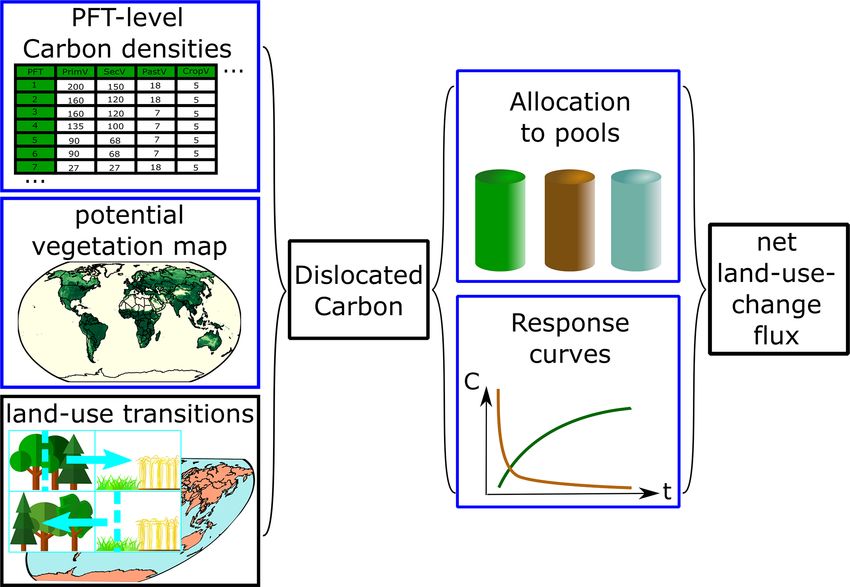
748    A. Bastos et al.: Comparison of uncertainties in land-use change fluxes from bookkeeping model parameterisation

Table 1. Summary of the most important characteristics of the two FLUC estimates from the two BK models used in the GCB2019 (BLUE
and HN2017), including how FLUC is calculated in the standard version and configuration of each model, the processes represented and how
they are parameterised. The model assumptions and parameterisations investigated in this study (see Table 2) are highlighted in bold.

                                                               BLUE                                 HN2017
                                 Spatial representation        Grid scale (0.25◦ × 0.25◦ )          Country/region level
                                 PFTs                          11 spatially explicit                20 per country
             FLUC calculation    LUC transitions               Gross                                Net
                                 Starting year                 850                                  1700
                                 Last year                     2018                                 2015
                                 Response curves               Exponential                          Exponential
                                 LUC transitions               LUH2v2h (Hurtt et al., 2020)         FAO (2015), FAOSTAT (2015)
                                 Shifting cultivation          Included explicitly                  Indirectly included (if FRA
                                                                                                    forest loss is larger than FAO
                                                                                                    agricultural expansion)
             Processes
                                 Harvest                       Three pools (1, 10, 100 years)       Three pools (1, 10, 100 years)
                                 Clearing                      Three pools (1, 10, 100 years)       Three pools (1, 10, 100 years)
                                                               plus slash                           plus slash
                                 Carbon densities              For each of the 11 PFTs based        Per country and for each of
                                 (Cdens)                       (vegetation and soil)                the 20 PFTs (vegetation);
                                                               on Houghton et al. (1983)            only per PFT (soil)
             Parameters          Decay times for the           For each of the 11 PFTs              For each of the 20 PFTs
                                 response curves (RCt)
                                 Pool allocation fractions     Different allocation                 Different allocation fractions
                                 (Alloc)                       fractions for each of the            per country and for each of
                                                               11 PFTs                              the 20 PFTs

Table 2. Selected settings in the simulations conducted with BLUE. The row in bold highlights the reference simulation.

                                             Starting     Transitions   C densities    Carbon         Response
                                                 year                   (Cdens)        allocation     curves
                                                                                       (Alloc)        decay
                                                                                                      times (t)
                                SBL               850     Gross         BLUE           BLUE           BLUE
                                SBL-Net          1700     Net           BLUE           BLUE           BLUE
                                SHNCdens         1700     Net           HN2017         BLUE           BLUE
                                SHNAlloc         1700     Net           BLUE           HN2017         BLUE
                                SHNt             1700     Net           BLUE           BLUE           HN2017
                                SHNFull          1700     Net           HN2017         HN2017         HN2017

      simulation, net land conversion is taken first from pri-                  nal forcing (LUH2v2.1 in BLUE as compared to FAO in
      mary land; i.e. abandonment (to secondary land) is al-                    HN2017). All subsequent simulations are run with this
      lowed to cancel clearing from preferentially primary                      setup but with different parameterisations (Table 2).
      land in addition to secondary land, which reduces emis-
      sion estimates more than if abandonment were allowed                   – In SHNCdens , BLUE is run using the C densities in veg-
      to cancel clearing only of secondary land (Hansis et                     etation and soil parameters from HN2017. Although
      al., 2015). The choice for net transition implementation                 C density parameters in HN2017 are defined on a per-
      aims to make FLUC estimates more comparable to the                       country and per-PFT basis, only vegetation C densi-
      approach in HN2017, albeit keeping the different origi-                  ties differ between countries for a given PFT, while

Earth Syst. Dynam., 12, 745–762, 2021                                                           https://doi.org/10.5194/esd-12-745-2021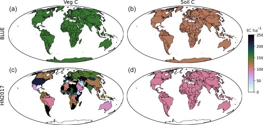
A. Bastos et al.: Comparison of uncertainties in land-use change fluxes from bookkeeping model parameterisation                          749

Figure 1. Schematic description of the BLUE model set up and of the changes made in each of the factorial simulations (highlighted in blue
boxes and summarised in Table 2). The model is forced by a map of grid-cell-level land-use transitions occurring at time t (gross vs. net).
These are then combined with a potential vegetation map of 11 natural vegetation types (Table A1), each having specific carbon densities
in vegetation and soil pools (Cdens), to calculate the carbon dislocated by each transition. The mass of dislocated carbon is then distributed
among different slash and product pools (Alloc), with specific response curves with different decay times (t).

     soil C densities only differ per PFT (for example, for                 – In SHNt , the decay times from HN2017 are used in
     tropical evergreen broadleaved forest in Fig. A1). The                   BLUE.
     global average values per PFT for BLUE and HN2017
     are given in Table A2. BLUE has generally higher veg-                  – In SHNFull , BLUE is run using net LUC transitions, start-
     etation and soil C densities in the tropics and most tem-                ing in 1700 and using HN2017 parameters for C den-
     perate PFTs, and lower vegetation and soil C densities in                sities, harvest and clearing allocation fractions and de-
     pastures, and lower soil C densities in croplands, com-                  cay times (i.e. a combination of SHNCdens , SHNAlloc and
     pared to the average values of HN2017.                                   SHNt ).

  – In SHNAlloc , BLUE is run using the harvest and clearing                In those simulations where BLUE is run with all or a sub-
    allocation fractions, and the slash fractions following              set of HN2017 parameters (SHNCdens , SHNAlloc , SHNt ), in-
    clearing from HN2017, but the C densities in vegeta-                 stead of global values per PFT, the values per PFT from
    tion and soil from BLUE. The global average values for               HN2017 are translated into BLUE PFTs and organised into
    BLUE and HN2017 are given in Table A3. In the actual                 parameter maps that can be read by BLUE. The difference
    HN2017 model run (Houghton and Nassikas, 2017), the                  between these simulations and SBL-NET provides an esti-
    allocations vary over time. Since BLUE uses tempo-                   mate of FLUC differences each including one set of param-
    rally static fractions, we used an average over the full             eters from HN2017 in BLUE. For SHNFull , the difference
    period (1850–2015). Harvest slash fractions in BLUE                  with SBL-NET is not expected to be simply the sum of the cor-
    (with timescales of 5–15 years in BLUE) are larger in                responding SHNCdens , SHNAlloc and SHNt differences because
    BLUE than in HN2017 for all PFTs. HN2017 allocates                   of interactions between C densities, allocation fractions and
    more harvest product to the long-lived pool over the pe-             response times, with differences in model structure and LUC
    riod 1850–2015 than BLUE (Table A3). For clearing,                   forcing, as described in Fig. 1.
    the short and long-lived pools are relatively similar be-
    tween the models but the medium-lived pool is larger in
                                                                         2.3    Model comparison
    BLUE, depending however on the PFT considered. The
    slash fractions following clearing from HN2017 are also              We calculate FLUC from the different simulations be-
    used instead of those in BLUE.                                       tween 1850 and 2015 (the period common to both datasets)
                                                                         for the globe and for the 18 regions used in Bastos et

https://doi.org/10.5194/esd-12-745-2021                                                       Earth Syst. Dynam., 12, 745–762, 2021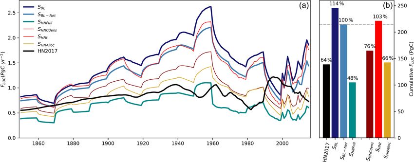
750     A. Bastos et al.: Comparison of uncertainties in land-use change fluxes from bookkeeping model parameterisation

al. (2020) to evaluate sources of uncertainty in land car-             All BLUE simulations show similar interannual variabil-
bon budgets: Canada (CAN), USA, central America (CAM),              ity patterns, consistent with the use of the LUH2v2.1 forc-
northern South America (NSA), Brazil (BRA), southern                ing, but these variations are dampened when the parame-
South America (SSA), Europe (EU), northern Africa (NAF),            ters for C densities, allocation fractions and time constants
equatorial Africa (EQAF), southern Africa (SAF), the Mid-           from HN are used. The BLUE simulation using the full set
dle East (MIDE), Russia (RUS), the Korean Peninsula and             of HN2017 parameters (SHNFull ) shows FLUC close to those
Japan (KAJ), central Asia (CAS), China (CHN), southern              of HN2017 until the 1980s and with a weak peak in emis-
Asia (SAS), SE Asia (SEAS) and Oceania (OCE). We then               sions in 1960s and relatively stable FLUC rather than an in-
evaluate separately the contribution of running BLUE with           creasing trend in 2000–2015. The resulting cumulative FLUC
the reference HN2017 setup, i.e. with net instead of gross          for SHNFull is 104 PgC, 52 % lower than SBL-NET , at the low
transitions and starting in the 1700s (SBL-Net –SBL ). SBL-Net is   end of previous estimates (Hansis et al., 2015; Houghton et
then used as the baseline for comparison with other simula-         al., 2012). This value is substantially outside the cumulative
tions, which follow the same setup (net emissions in simula-        budget range of the GCB2019 (205±60 PgC 1850–2018) but
tions starting in 1700).                                            still consistent with the uncertainty range of ±0.7 PgC yr−1
   Both BLUE and HN2017 add emissions from peat burn-               provided by GCB2019 after 1959.
ing (van der Werf et al., 2017) and drainage (Hooijer et al.,          The parameters that lead to larger differences in
2010) in a post-processing step. For easier comparison of di-       global FLUC are the C densities (SHNCdens , Fig. 2, dark red)
rect model output, we do not include these post-processing          and the allocation rules (SHNAlloc , yellow), while chang-
steps.                                                              ing the decay times have small effect. Both SHNCdens and
   For all simulations, we compare both the interannual vari-       SHNAlloc result in lower FLUC over the 1850–2015 period,
ability in FLUC and the resulting cumulative emissions be-          and weaker increasing trends between 2000 and 2015, which
tween 1850 and 2015. The discrepancies in interannual vari-         indicates that the trends in this period are not only due to
ability of estimated FLUC between HN2017 and each simu-             forcing differences (Bastos et al., 2020) but in part from
lation from BLUE (Si ) are assessed by the root mean square         model parameterisation. The cumulative FLUC in 1850–2015
difference of FLUC from each simulation, calculated as              is 164 and 142 PgC for SHNCdens and SHNAlloc respectively,
                      v
                      uN                                            i.e. 24 % and 34 % lower than SBL-Net , and closer to the
                      u (HN2017i − Si )2
                      uP                                            HN2017 estimate on global scale. The lower FLUC with
                      t i                                           HN2017 C densities can be explained by the HN2017 lower
RMSDHN-BLUE-i =                              ,               (1)
                                  N                                 C densities in both vegetation and soil for most PFTs and
where N is the number of years. In addition, we compare the         the smaller difference between primary and secondary for-
effect of the different parameterisations on the gross LUC          est C stocks (Table A2) compared to BLUE. In particular,
fluxes: fluxes from clearing of primary or secondary natural        BLUE often features higher vegetation carbon in broadleaf
vegetation, wood harvest (net of decay and regrowth), aban-         forests and higher soil carbon in most other ecosystems than
donment of agricultural land (cropland and pasture) and tran-       HN2017, which, together with lower soil carbon assumed
sitions between cropland and pasture.                               for cropland and pasture, leads to substantially larger carbon
                                                                    losses in BLUE for many transitions (Table A2). Even though
                                                                    SHNt results in a small positive difference in cumulative FLUC
3     Results
                                                                    relative to SBL-NET (221 PgC), effect of response-curve times
                                                                    is multiplicative (Fig. 1), therefore the FLUC trends are am-
3.1    Global FLUC
                                                                    plified (Fig. 2, left panel).
We analyse annual FLUC from 1850 until 2015 (Fig. 2, left
panel). The BLUE simulation for GCB2019 (SBL , dark blue            3.2   Regional patterns
line) estimates higher emissions from LUC than HN2017
(black line). The cumulative emissions between 1850–                The global differences between simulations result from inter-
2015 (Fig. 2, right panel) are 139 PgC for HN2017 and               actions between the different factors and in the types of LUC
245 PgC for SBL . SBL-Net shows lower FLUC , but results            occurring in a given point in space and time. We first analyse
in cumulative emissions only approximately 13 % lower               the temporal evolution of regional FLUC for each simulation
(214 PgC) than when using gross transitions. As in previ-           (Fig. 3).
ous BLUE estimates, both SBL and SBL-Net show an increase              The factorial analysis sheds light on the underlying rea-
in FLUC from 1850 until the mid-20th century, peaking at            sons of the diverging trends in the 2000s, where BLUE
around 1960 and then decreasing sharply until the 1990s,            showed an upward trend, opposing the downward trend
while HN2017 shows less variability. The two datasets fur-          in FLUC from HN2017. In absolute terms, the upward trend
ther show contrasting trends from around 1975 until 2015,           in BLUE stems foremost from BRA (a peak of about
with BLUE increasing sharply after the late 1990s, when             0.45 PgC yr−1 in the early 2000s, then a decline; similar
HN2017 shows a decrease.                                            in HN2017 but peaking at about 0.3 PgC yr−1 ), SSA (also

Earth Syst. Dynam., 12, 745–762, 2021                                                 https://doi.org/10.5194/esd-12-745-2021
A. Bastos et al.: Comparison of uncertainties in land-use change fluxes from bookkeeping model parameterisation 751 Figure 2. Global FLUC between 1850 and 2015 (a) from the two bookkeeping model estimates in GCB2019 (HN2017 in black and SBL for BLUE in dark blue), the BLUE simulations with net LUC transitions and standard BLUE parameterisation (light blue, SBL-Net , used as reference for all subsequent BLUE runs) and using all tested HN2017 parameterisations together (cyan, SHNFull ). The factorial simulations with only one set of parameters changed are shown in thin lines (SHNCdens in dark red, SHNt in red, SHNAlloc in yellow). The corresponding cumulative totals between 1850 and 2015 are shown in panel (b), and values relative to SBL-Net are shown by the numbers above bars. captured by HN2017 but accelerating from the 2000s to et al., 2017; Fuchs et al., 2015). However, this increases the 2010s in BLUE, decelerating in HN2017), NAF (by the RMSDHN-BLUE by only 2 TgC yr−1 . comparison more stable in HN2017), EQAF (similar val- As seen for global FLUC , the simulation using HN2017 pa- ues as in HN2017 but with 0.15 PgC yr−1 FLUC in BLUE rameter values (SHNFull ) leads to a reduction of FLUC by 50 % in the 1970s–2000s is only about half that of HN2017) and or more compared to SBL in many regions (dark blue colours, SEAS (where HN2017 has a peak in the 1990s, then a steep see values in the centre of grid cells in Fig. 4a), except for drop of 0.3 PgC yr−1 to 2015, while BLUE FLUC picks up CAS, where an increase of 47 % is estimated, mainly due to by about 0.2 PgC yr−1 over the 2000s). Additionally, BLUE differences in C density parameters. The reductions in cumu- shows an increase in FLUC in CHN for the 2010s, while lative FLUC differences in CAM, BRA, EU and SEAS. De- HN2017 estimates a sink due to afforestation. In all of these creases in the RMSDHN-BLUE between SHNFull and SBL-Net regions, adjusting BLUE partly or fully to HN2017 param- globally and for 11 of the 18 regions (Fig. 4b), with small eters does not obviously bring trends closer together, be- increases elsewhere. This shows that differences in setup and cause a lowering of the 2000s FLUC in BLUE, which re- parameterisation cancel differences arising from the differ- sults from several of the factorial experiments, would lead ent land-use forcing in BLUE and HN2017 in some regions. to lower FLUC in earlier time periods as well. In addition, the reductions in RMSDHN-BLUE in SHNFull To summarise these patterns, we calculate the relative av- compared to SBL are stronger than for SBL-Net , indicating erage differences in regional cumulative FLUC from SBL-Net that parameterisation differences have stronger contribution and SHNFull with SBL (top panel of Fig. 4a, values in per- to RMSDHN-BLUE than the impact of simulation net/gross cent change) and the root mean square difference with transitions. HN2017 (Eq. 1, RMSDHN-BLUE ), which reflects differences The differences between SBL-Net and each of the factorial in interannual variability (top panel of Fig. 4b, in TgC yr−1 ). simulations (bottom panel of Fig. 4a) shows that C densi- Even though SBL-Net results in a small (−13 %) decrease ties and allocation rules are the dominant factors not just in global FLUC compared to SBL as discussed above, regional for global FLUC , but also in most regions, and lead to differences show stronger decreases, especially in regions lower RMSDHN-BLUE , compared to SBL-Net (Fig. 4b). Using with intensive shifting cultivation practices, such as SEAS HN2017 allocation fractions to pools for harvest and clear- (−40 %), CAM (−22 %), SAF and EQAF (−23 % in both). ing results in lower cumulative FLUC everywhere (SHNAlloc ) SBL-Net additionally leads to higher agreement in interannual and decreases the RMSDHN-BLUE at global scale and in all variability with HN2017 at global scale but also for most regions but NSA and SSA. Altering C densities (SHNCdens ) regions (i.e. lower RMSDHN-BLUE , Fig. 4b). Europe shows has contrasting effects in cumulative FLUC between regions, 7 % higher cumulative FLUC for SBL-Net than SBL , likely increasing cumulative FLUC in 3 out of 18 regions. Strong because of the importance of subpixel post-abandonment reductions in RMSDHN-BLUE for SHNFull are found in BRA, recovery and re-/afforestation dynamics in Europe (Bayer RUS, CHN and SAS (top panel in Fig. 4b), explained https://doi.org/10.5194/esd-12-745-2021 Earth Syst. Dynam., 12, 745–762, 2021
752    A. Bastos et al.: Comparison of uncertainties in land-use change fluxes from bookkeeping model parameterisation

Figure 3. Regional FLUC between 1850 and 2015 from the two BK model estimates in GCB2019 (HN2017 in black and SBL for BLUE in
dark blue), the BLUE simulations with net LUC transitions and standard parameterisation (light blue, SBL-Net ) and using HN2017 parame-
terisations (cyan, SHNFull ). The factorial simulations with only one set of parameters changed are shown in thin lines (SHNCdens in dark red,
SHNt in red, SHNAlloc in yellow).

by RMSDHN-BLUE reductions by changing the C densities in                 tions between different parameters to the overall FLUC vari-
vegetation and soil pools (SHNCdens ) and allocation fractions.          ability. The decay times generally contribute to small in-
In SEAS, cumulative FLUC is reduced when using HN2017                    creases in cumulative FLUC compared to SBL-Net , except
parameters (SHNFull ) but with a higher RMSDHN-BLUE . In                 NAF where they increase FLUC by 22 % and would slightly
this region, C density parameters contribute the most to the             amplify RMSDHN-BLUE globally and in 13 of the 18 regions.
reduction of bias, compared to SBL-Net , and both C density
parameters and allocation fractions contribute to the increase
in RMSDHN-BLUE . This highlights the importance of interac-

Earth Syst. Dynam., 12, 745–762, 2021                                                         https://doi.org/10.5194/esd-12-745-2021
A. Bastos et al.: Comparison of uncertainties in land-use change fluxes from bookkeeping model parameterisation                    753

Figure 4. (a) Relative changes in cumulative simulated FLUC between 1850–2015 for each region for SBL-Net and SHNFull compared to SBL
(top two rows) and the relative effect of each parameter change, compared to SBL-NET (bottom three rows) indicated by the colours and
numbers in the centre of cells. (b) The RMSDHN-BLUE for each simulation indicated by the colours and numbers in the centre of cells. All
panels show results for the period 1850–2015.

3.3   Effects on gross FLUC component fluxes                          tive and negative differences are found. The lower FLUC from
                                                                      clearing to agriculture for SHNFull in most grid cells is linked
To better understand the effects of the different parame-             with the lower vegetation and soil C densities for most for-
terisations on FLUC , we analyse the spatial distribution of          est PFTs (Table A2). Higher FLUC from wood harvest are
the differences between SHNFull , SHNCdens , SHNAlloc , SHNt          simulated by SHNFull in eastern and northern North Amer-
and SBL-Net decomposed into gross FLUC : fluxes from har-             ica, central Europe and Scandinavia and China, mostly re-
vest, clearing, abandonment/regrowth and transitions be-              lated with response-curve time constants. Other transitions
tween crop and pasture (Fig. 5).                                      (crop to pasture or pasture to crop) result in higher FLUC
   In most grid cells, the difference between SHNFull and             for SHNFull in most semi-arid regions, which is explained to a
SBL-Net is dominated by the effects of the parameterisation           larger extent by differences in C densities and time constants
of C densities in gross fluxes and allocation rules for aban-         between the two models (SHNCdens , SHNt ) than by allocation
donment fluxes. For FLUC from abandonment and clearing                rules (SHNAlloc ) (Table A2).
to agriculture (crop and pasture), the differences are mostly
negative (i.e. higher uptake from recovery and lower emis-            4   Discussion
sions from clearing to agriculture using HN2017 parameter-
isation), while for the fluxes from transitions between crop          Fluxes from land-use change and management are one of
and pastures and harvest, regional contrasts between posi-            the most uncertain and least constrained components of the

https://doi.org/10.5194/esd-12-745-2021                                                   Earth Syst. Dynam., 12, 745–762, 2021
754 A. Bastos et al.: Comparison of uncertainties in land-use change fluxes from bookkeeping model parameterisation Figure 5. Spatial distribution of relative differences in average FLUC between 1850–2018 for each of the four simulations with HN2017 parameters (SHNFull , SHNCdens , SHNAlloc , SHNt ), compared to SBL-Net for different FLUC components: wood harvest, abandonment, clearing and crop–pasture transitions. Regions with average low values of FLUC (e.g. deserts) are masked. global carbon cycle (Bastos et al., 2020; Friedlingstein et same rule. Cancelling of primary and secondary land clear- al., 2019; Houghton, 2020). Several sources of uncertainty ing, with primary first, gave 24 % lower emissions in Hansis in FLU C have been previously analysed, such as the choice et al. (2015). The differences are likely explained by the sub- of gross vs. net LUC transitions (Bayer et al., 2017; Fuchs et stantial changes that came in with the change from LUH1 al., 2015; Gasser et al., 2020; Wilkenskjeld et al., 2014), the to LUH2 versions, in particular the change to Heinimann et definitions and terminology used (Grassi et al., 2018; Pon- al. (2017) shifting cultivation maps. gratz et al., 2014) or the management processes considered Based on observation-based constraints by atmospheric in- (Arneth et al., 2017; Pugh et al., 2015). The two bookkeep- versions Bastos et al. (2020) pointed out that FLUC estimated ing models used in the global carbon budgets may differ in by DGVMs and BLUE in BRA, SEAS, EU and EQAF were their FLUC estimates due to differences in the forcing data probably too high. Our analysis shows that FLUC estimates and differences in model structure, parameterisation and in for these regions, except EU would be lower if the setup of how certain processes are represented. The impact of the HN2017 were used, i.e. starting in 1700 instead of 850 and LUC forcing on FLUC has been extensively investigated in using net transitions, and all four regions would show even previous studies (Bastos et al., 2020; Gasser et al., 2020; Har- larger reductions in FLUC if the parameterisation of HN2017 tung et al., 2021). Both models have a similar structure (Ta- were used in BLUE. However, these changes would also ble 2) and both models use parameters from different sources bring down FLUC estimates in many regions that were not that are based on observations which are, however, uncertain. deemed too high in FLUC based on the constraint by obser- Here, we evaluate how the different model parameterisations vations. This suggests that neither the BLUE nor HN2017 impact FLUC estimates and whether they can explain differ- setup and parameterisation can be judged as being superior ences in global and regional average FLUC and on variability to the other for all regions of the world and all time periods. between the two models since 1850. The rules for allocation of displaced carbon to different The simulation with net transition (SBL-Net ) reduces differ- pools have the strongest effect on average FLUC , as well as ences in the average and interannual variability of FLUC es- their variability, followed by C density parameters. Contrary timates from BLUE and HN2017. The contribution of gross to C densities (Sect. 4.1), at the moment no global dataset to FLUC is smaller than previous estimates (15 %–38 %, Ar- of allocation parameters exists that could be compared to neth et al., 2017; Fuchs et al., 2015; Hansis et al., 2015) and the allocation fractions used here. BLUE and HN2017 FLUC also lower than in earlier BLUE simulations that used the in 1850–2015 show better agreement in temporal variability, Earth Syst. Dynam., 12, 745–762, 2021 https://doi.org/10.5194/esd-12-745-2021
A. Bastos et al.: Comparison of uncertainties in land-use change fluxes from bookkeeping model parameterisation                    755

mostly because fact that the C density and allocation param-
eterisations of HN2017 dampen the effect of differences in
land-use change transitions.
   This elimination of the 2000s trend difference in some re-
gions comes at the cost of larger divergences in earlier times.
With high LUC dynamics in the 20th century in some re-
gions, which is more strongly captured by BLUE with its
representation of gross transitions, slightly larger C density
losses with the transformation of natural vegetation to agri-
culture or degradation by wood harvesting and rangelands
may lead to an increase in FLUC beyond what would be ex-
pected from net land-use areas alone. On top comes a distri-
bution of cleared and harvested material to faster pools (more
slash in BLUE, more long-lived products in HN2017), which
also emphasises the effects of LUC dynamics. The differ-
ences between BLUE and HN2017 are thus a combination
of higher LUC dynamics in BLUE (by using LUH2v2.1 and              Figure 6. Carbon stocks in vegetation (y axis) and soils (x axis)
                                                                   simulated by BLUE for the pre-industrial period (1850, big circles)
accounting for gross transitions) and of faster material decay
                                                                   and present time (2018, small circles, end of arrows). These values
than in HN2017. The different trends of BLUE and HN2017
                                                                   are compared to two observation-based reference datasets: that of
in the 1950s and after 1990 are instead largely attributable to    Anav et al. (2013) for both vegetation and soil carbon stocks (black
the different LUC forcing (Gasser et al., 2020).                   square) and the upper and lower values of potential (solid lines) and
                                                                   present-day (dashed lines) carbon stocks in vegetation from Erb et
4.1   Constraining C densities                                     al. (2018).

The parameterisation of C densities of vegetation and soil
pools is the second most relevant parameter but one that af-
                                                                   Additionally, these simulations result in present-day C stocks
fects all flux components. Even though both models were
                                                                   in vegetation that are within the range provided by Erb et
parameterised based on observation-based C densities, these
                                                                   al. (2018), or close to its upper limit, and are also consistent
parameters are highly uncertain, as they are derived from
                                                                   with the reference value from Anav et al. (2013). All simula-
sparse plot-level data with high variance across datasets
                                                                   tions estimate lower C stocks in the soil, compared to Anav
(Brown and Lugo, 1982; Post et al., 1982; Schlesinger,
                                                                   et al. (2013). HN2017 has higher C stocks in soil both for the
1984; Zinke et al., 1986). Remote-sensing-based estimates
                                                                   pre-industrial period and the present day, compared to BLUE
of potential vegetation C stocks in undisturbed lands and
                                                                   simulations, which are close to the values estimated by Anav
well as present-day C stocks have been produced by Erb
                                                                   et al. (2013). The two simulations using HN2017 carbon den-
et al. (2018), including their uncertainty. The values of Erb
                                                                   sities (SHNFull , and SHNCdens ) result in too-low C stocks in
et al. (2018) can, therefore, be compared to the potential
                                                                   soils, compared to Anav et al. (2013), and much lower po-
C stocks simulated by HN2017 and by BLUE using the dif-
                                                                   tential vegetation C stocks than Erb et al. (2018). However,
ferent configurations in this study (circles in Fig. 6), as well
                                                                   present-day vegetation C stocks for SHNFull and SHNCdens are
as of simulated present-day carbon stocks (small circles, end
                                                                   consistent with their values.
of arrows). In addition, we compare simulated C stocks with
those of Anav et al. (2013) for the present day.
    All BLUE simulations, as well as HN2017, have 4 %–6 %
lower potential C stocks in vegetation than estimates in Erb       5   Conclusions
et al. (2018) (Fig. 6). Since the values of potential biomass
in Erb et al. (2018) were estimated for present day, they in-      We conclude that differences between BLUE and HN2017
clude the effect of environmental changes such as CO2 fer-         arise from the higher allocation of cleared and harvested ma-
tilisation, and are expected to be up to 10 % higher than they     terial to quickly decomposing pools in BLUE, compared to
would be without these effects (Pongratz et al., 2014). There-     HN2017, combined with higher emissions in BLUE due to
fore, the C stocks in vegetation simulated both by BLUE and        often larger differences in soil and vegetation C densities be-
HN2017 are consistent with these remote-sensing based es-          tween natural and managed vegetation or primary and sec-
timates, if environmental effects are excluded. The method-        ondary vegetation. It should be noted, however, that spe-
ology of using the highest percentiles in a moving window          cific transitions and prevalence of specific PFTs in certain
as a potential value in Erb et al. (2018) could overestimate       regions prohibits generalising this statement. Together with
biomass because it has a bias towards capturing the oldest         the larger land-use dynamics which stem from BLUE repre-
rather than average forests in a cycle of natural disturbances.    senting gross transitions and its usage of LUH2v2.1 as LUC

https://doi.org/10.5194/esd-12-745-2021                                                 Earth Syst. Dynam., 12, 745–762, 2021
756 A. Bastos et al.: Comparison of uncertainties in land-use change fluxes from bookkeeping model parameterisation forcing, these changes lead to overall higher carbon losses Similarly, improvements in allocation can be performed. that have a faster decay. Bookkeeping models, and many DGVMs, follow very sim- The two reference datasets of global C stocks seem to ple assumptions of the fate of cleared or harvested material, support the choice of C densities used in the default BLUE often along the lines of the “Grand Slam Protocol” (McGuire configuration and therefore the higher estimates of FLUC et al., 2001) but developed for bookkeeping models earlier by BLUE. However, it should be noted that both models (Houghton et al., 1983), which distinguishes only three prod- have limited representation of spatial variability in C den- uct pools (fast, medium, slow), with timescales defined rather sities: BLUE ignores spatial variability in vegetation and ad hoc as 1, 10 or 100 years. The fractions going into these soil C within each PFT distribution, for example, due to and into slash are compiled from individual studies for spe- less favourable climate in some regions; HN2017 includes cific regions (Houghton et al., 1983; Hurtt et al., 2020) but country-specific C densities for vegetation, but not for soil, are hard to quantify on the global level throughout several and no spatial variability within each country. centuries. Such long timescales are needed, however, to cap- The large contribution of the C densities to the differences ture the slow dynamics of decay and regrowth and thus to between the FLUC estimates of the two BK models found in capture legacy fluxes accurately. For the last decades, how- our results highlights the importance of deriving spatially ex- ever, more detailed data have become available than those plicit maps of vegetation, and soil C densities discriminated currently used in the models of the global carbon budgets, per vegetation type would be required. Producing such maps such as global sets of dynamic carbon-storage factors (Ma- is challenging, especially for the estimates of C densities in son Earles et al., 2012) that define a larger number of product undisturbed land, as most of the land surface has been di- pools and time-varying fractions of allocation. rectly or indirectly impacted by human activity. However, observation-based maps of vegetation and soil C densities in both disturbed and undisturbed land would be highly valu- able, as they could be used in BK models to reduce uncer- tainties in FLUC . Earth Syst. Dynam., 12, 745–762, 2021 https://doi.org/10.5194/esd-12-745-2021
A. Bastos et al.: Comparison of uncertainties in land-use change fluxes from bookkeeping model parameterisation           757

Appendix A

Table A1. Plant functional types in HN2017 and in BLUE, and the correspondence used in this study.

                                HN2017                     BLUE
                                Tropical rainforest        Tropical evergreen forest
                                Tropical moist deciduous   Tropical deciduous forest
                                Tropical dry forest
                                Tropical shrub             Raingreen shrubs
                                Tropical desert
                                Tropical mountain          Tropical evergreen forest
                                Subtropical humid forest   Temperate evergreen broadleaf forest
                                Subtropical dry forest     Temperate/boreal deciduous broadleaf forest
                                Subtropical steppe         C4 natural grasses
                                Subtropical desert
                                Subtropical mountain       Temperate/boreal evergreen conifers
                                Temperate oceanic          Temperate/boreal evergreen conifers
                                Temperate continental      Temperate/boreal deciduous broadleaf forest
                                Temperate steppe           C3 natural grasses
                                Temperate desert
                                Temperate mountain         Temperate/boreal deciduous broadleaf forest
                                Boreal coniferous          Temperate/boreal evergreen conifers
                                Boreal tundra              Tundra
                                Boreal mountain
                                Polar                      Tundra

https://doi.org/10.5194/esd-12-745-2021                                                  Earth Syst. Dynam., 12, 745–762, 2021
A. Bastos et al.: Comparison of uncertainties in land-use change fluxes from bookkeeping model parameterisation
https://doi.org/10.5194/esd-12-745-2021
Table A3. Global median values of harvest and clearing allocation rules to the short-, medium- and long-lived pools (1, 10 and 100 years) for BLUE PFTs, from the standard BLUE
setup and used for the simulations with parameters from HN2017 (converted to BLUE PFT classes). The slash fraction from clearing is calculated as the 1 minus the sum of the 1-,
10- and 100-year pools.
Slash primary Slash secondary Harvest Harvest Harvest Clearing Clearing Clearing
forest forest pool 1 pool 10 pool 100 pool 1 pool 10 pool 100
BLUE HN2017 BLUE HN2017 BLUE HN2017 BLUE HN2017 BLUE HN2017 BLUE HN2017 BLUE HN2017 BLUE HN2017
Tropical evergreen forest 0.79 0.5 0.71 0.5 0.90 0.49 0.04 0.11 0.06 0.40 0.4 0.42 0.27 0.01 0 0.08
Tropical deciduous forest 0.86 0.5 0.81 0.5 0.90 0.49 0.04 0.11 0.06 0.40 0.4 0.42 0.27 0.01 0 0.08
Temperate evergreen broadleaf forest 0.81 0.5 0.75 0.5 0.40 0.49 0.24 0.11 0.36 0.40 0.4 0.42 0.2 0.01 0.07 0.08
Temperate/boreal deciduous broadleaf forest 0.78 0.5 0.7 0.5 0.40 0.49 0.24 0.11 0.36 0.40 0.4 0.42 0.2 0.01 0.07 0.08
Temperate/boreal evergreen conifers 0.87 0.5 0.82 0.5 0.40 0.49 0.24 0.11 0.36 0.40 0.4 0.42 0.2 0.01 0.07 0.08
Temperate/boreal deciduous conifers 0.87 0.5 0.82 0.5 0.40 0.49 0.24 0.11 0.36 0.40 0.4 0.42 0.2 0.01 0.07 0.08
Raingreen shrubs 0.86 0.5 0.81 0.5 1.00 0.49 0.00 0.11 0.00 0.40 0.4 0.42 0.1 0.01 0 0.08
Summergreen shrubs 0.78 0.5 0.7 0.5 1.00 0.49 0.00 0.11 0.00 0.40 0.4 0.42 0.1 0.01 0 0.08
C3 natural grasses 0.78 0.5 0.7 0.5 1.00 0.49 0.00 0.11 0.00 0.40 0.5 0.42 0 0.01 0 0.08
C4 natural grasses 0.86 0.5 0.81 0.5 1.00 0.49 0.00 0.11 0.00 0.40 0.5 0.42 0 0.01 0 0.08
Tundra 0.87 0.5 0.82 0.5 1.00 0.49 0.00 0.11 0.00 0.40 0.42 0.4 0.01 0.1 0.08 0
Earth Syst. Dynam., 12, 745–762, 2021
134 101 178 204 160 204 178 204 5 1 7 7 11 0 14 3 Tundra
38 21 50 42 45 42 50 42 5 5 10 18 17 18 23 18 C4 natural grasses
60 94 80 189 72 189 80 189 3 5 10 7 17 7 23 7 C3 natural grasses
26 34 35 69 32 69 35 69 5 5 10 7 28 27 37 27 Summergreen shrubs
26 34 35 69 32 69 35 69 5 5 10 18 28 27 37 27 Raingreen shrubs
137 103 182 155 164 185 182 206 5 5 10 7 83 68 110 90 Temperate/boreal deciduous conifers
137 103 182 155 164 185 182 206 5 5 10 7 83 68 110 90 Temperate/boreal evergreen conifers
108 67 143 101 129 120 143 134 5 5 10 7 64 100 86 135 Temperate/boreal deciduous broadleaf forest
90 67 120 101 108 120 120 134 5 5 10 7 103 120 138 160 Temperate evergreen broadleaf forest
75 58 100 88 90 88 100 117 5 5 10 18 69 120 92 160 Tropical deciduous forest
73 58 98 88 88 88 98 117 5 5 10 18 114 150 152 200 Tropical evergreen forest
HN2017 BLUE HN2017 BLUE HN2017 BLUE HN2017 BLUE HN2017 BLUE HN2017 BLUE HN2017 BLUE HN2017 BLUE
soil C soil C soil C soil C veg C veg C veg C veg C
Crop Pasture Secondary Primary Crop Pasture Secondary Primary
PFT classes as used for the simulations with parameters from HN2017. Units are tC ha−1 .
Table A2. Global median value across countries per PFT for vegetation C densities and PFT-dependent soil C densities from BLUE, and from HN2017 converted to BLUE
758A. Bastos et al.: Comparison of uncertainties in land-use change fluxes from bookkeeping model parameterisation 759 Figure A1. Carbon densities in vegetation (a, c) and soil (b, d) for tropical broadleaved evergreen forests for BLUE (a, b) and HN2017 (c, d) in tC ha−1 . It should be noted that even though C density values are assigned on a per-country basis in HN2017, they do not differ between countries for soil C. Note that C densities are assigned to all countries, even if evergreen broadleaved forest is not present in a given country. https://doi.org/10.5194/esd-12-745-2021 Earth Syst. Dynam., 12, 745–762, 2021
760     A. Bastos et al.: Comparison of uncertainties in land-use change fluxes from bookkeeping model parameterisation

Code availability. The bookkeeping model code can be requested          References
from Richard A. Houghton (HN2017) and Julia Pongratz (BLUE).
Other scripts are available upon request to the corresponding author.
                                                                        Anav, A., Friedlingstein, P., Kidston, M., Bopp, L., Ciais, P., Cox,
                                                                           P., Jones, C., Jung, M., Myneni, R., and Zhu, Z.: Evaluating the
Data availability. The global and regional fluxes from HN2017              Land and Ocean Components of the Global Carbon Cycle in
and the BLUE simulations are provided in the Supplement. The               the CMIP5 Earth System Models, J. Climate, 26, 6801–6843,
gridded fields of the BLUE simulations can be provided by the con-         https://doi.org/10.1175/JCLI-D-12-00417.1, 2013.
tact author upon request.                                               Arneth, A., Sitch, S., Pongratz, J., Stocker, B., Ciais, P., Poulter, B.,
                                                                           Bayer, A., Bondeau, A., Calle, L., Chini, L. P., Gasser, T., Fader,
                                                                           M., Friedlingstein, P., Kato, E., Li, W., Lindeskog, M., Nabel, J.
                                                                           E. M. S., Pugh, T. A. M., Robertson, E., Viovy, N., Yue, C., and
Supplement. The supplement related to this article is available
                                                                           Zaehle, S.: Historical carbon dioxide emissions caused by land-
online at: https://doi.org/10.5194/esd-12-745-2021-supplement.
                                                                           use changes are possibly larger than assumed, Nat. Geosci., 10,
                                                                           79–84, https://doi.org/10.1038/ngeo2882, 2017.
                                                                        Bastos, A., Ciais, P., Barichivich, J., Bopp, L., Brovkin, V., Gasser,
Author contributions. AB designed the study together with JP,              T., Peng, S., Pongratz, J., Viovy, N., and Trudinger, C. M.: Re-
with input from KH, JEMSN and TBN. AB planned and executed                 evaluating the 1940s CO2 plateau, Biogeosciences, 13, 4877–
the model simulations as well as the overall analysis. RAH and             4897, https://doi.org/10.5194/bg-13-4877-2016, 2016.
JP provided expert knowledge on each of the two bookkeeping             Bastos, A., O’Sullivan, M., Ciais, P., Makowski, D., Sitch, S.,
models. TBN prepared Fig. 1. KH, JP, RAH and JEMSN con-                    Friedlingstein, P., Chevallier, F., Rödenbeck, C., Pongratz, J.,
tributed to the discussion of the results. AB prepared the original        and Luijkx, I.: Sources of uncertainty in regional and global
draft; all other co-authors participated in the review and editing of      terrestrial CO2 -exchange estimates, Global Biogeochem. Cy.,
the paper.                                                                 34, e2019GB006393, https://doi.org/10.1029/2019GB006393,
                                                                           2020.
                                                                        Bayer, A. D., Lindeskog, M., Pugh, T. A. M., Anthoni, P. M., Fuchs,
Competing interests. The authors declare that they have no con-            R., and Arneth, A.: Uncertainties in the land-use flux resulting
flict of interest.                                                         from land-use change reconstructions and gross land transitions,
                                                                           Earth Syst. Dynam., 8, 91–111, https://doi.org/10.5194/esd-8-
                                                                           91-2017, 2017.
Disclaimer. Publisher’s note: Copernicus Publications remains           Brown, S. and Lugo, A. E.: The Storage and Production
neutral with regard to jurisdictional claims in published maps and         of Organic Matter in Tropical Forests and Their Role
institutional affiliations.                                                in the Global Carbon Cycle, Biotropica, 14, 161–187,
                                                                           https://doi.org/10.2307/2388024, 1982.
                                                                        Di Vittorio, A. V., Shi, X., Bond-Lamberty, B., Calvin, K., and
Acknowledgements. We thank Andrea Castanho and Alexan-                     Jones, A.: Initial Land Use/Cover Distribution Substantially
der A. Nassikas for support in extracting parameters from the              Affects Global Carbon and Local Temperature Projections in
HN2017 model.                                                              the Integrated Earth System Model, Global Biogeochem. Cy.,
                                                                           34, e2019GB006383, https://doi.org/10.1029/2019GB006383,
                                                                           2020.
Financial support. The article processing charges for this open-        Erb, K.-H., Kastner, T., Plutzar, C., Bais, A. L. S., Carval-
access publication were covered by the Max Planck Society.                 hais, N., Fetzel, T., Gingrich, S., Haberl, H., Lauk, C.,
                                                                           Niedertscheider, M., Pongratz, J., Thurner, M., and Luys-
                                                                           saert, S.: Unexpectedly large impact of forest management
                                                                           and grazing on global vegetation biomass, Nature, 553, 73–76,
Review statement. This paper was edited by Zhenghui Xie and
                                                                           https://doi.org/10.1038/nature25138, 2018.
reviewed by two anonymous referees.
                                                                        FAO: Global Forest Resources Assessment 2015 (FRA2015), Food
                                                                           and Agriculture Organization of the United Nations, Rome,
                                                                           2015.
                                                                        FAOSTAT: FAOSTAT: Food and Agriculture Organization of the
                                                                           United Nations, Rome, Italy, 2015.
                                                                        Friedlingstein, P., Jones, M. W., O’Sullivan, M., Andrew, R. M.,
                                                                           Hauck, J., Peters, G. P., Peters, W., Pongratz, J., Sitch, S.,
                                                                           Le Quéré, C., Bakker, D. C. E., Canadell, J. G., Ciais, P., Jack-
                                                                           son, R. B., Anthoni, P., Barbero, L., Bastos, A., Bastrikov, V.,
                                                                           Becker, M., Bopp, L., Buitenhuis, E., Chandra, N., Chevallier,
                                                                           F., Chini, L. P., Currie, K. I., Feely, R. A., Gehlen, M., Gilfillan,
                                                                           D., Gkritzalis, T., Goll, D. S., Gruber, N., Gutekunst, S., Har-
                                                                           ris, I., Haverd, V., Houghton, R. A., Hurtt, G., Ilyina, T., Jain,
                                                                           A. K., Joetzjer, E., Kaplan, J. O., Kato, E., Klein Goldewijk, K.,

Earth Syst. Dynam., 12, 745–762, 2021                                                        https://doi.org/10.5194/esd-12-745-2021
You can also read