Using publicly available satellite imagery and deep learning to understand economic well-being in Africa
←
→
Page content transcription
If your browser does not render page correctly, please read the page content below
ARTICLE
                  https://doi.org/10.1038/s41467-020-16185-w                OPEN

                  Using publicly available satellite imagery
                  and deep learning to understand economic
                  well-being in Africa
                  Christopher Yeh             1,7,
                                                Anthony Perez             1,2,7,Anne Driscoll3, George Azzari2,4, Zhongyi Tang5, David Lobell3,4,5,
                  Stefano Ermon           1   & Marshall Burke           3,4,5,6 ✉
1234567890():,;

                  Accurate and comprehensive measurements of economic well-being are fundamental inputs
                  into both research and policy, but such measures are unavailable at a local level in many parts
                  of the world. Here we train deep learning models to predict survey-based estimates of asset
                  wealth across ~ 20,000 African villages from publicly-available multispectral satellite ima-
                  gery. Models can explain 70% of the variation in ground-measured village wealth in countries
                  where the model was not trained, outperforming previous benchmarks from high-resolution
                  imagery, and comparison with independent wealth measurements from censuses suggests
                  that errors in satellite estimates are comparable to errors in existing ground data. Satellite-
                  based estimates can also explain up to 50% of the variation in district-aggregated changes in
                  wealth over time, with daytime imagery particularly useful in this task. We demonstrate the
                  utility of satellite-based estimates for research and policy, and demonstrate their scalability
                  by creating a wealth map for Africa’s most populous country.

                  1 Department  of Computer Science, Stanford University, 353 Serra Mall, Stanford, CA 94305, USA. 2 AtlasAI, 459 Hamilton Ave, Palo Alto, CA 94301, USA.
                  3 Center on Food Security and the Environment, Stanford University, 616 Jane Stanford Way, Stanford, CA 94305, USA. 4 Department of Earth System
                  Science, Stanford University, 473 Via Ortega, Stanford, CA 94305, USA. 5 Stanford Institute for Economic Policy Research, Stanford University, 366 Galvez
                  St, Stanford, CA 94305, USA. 6 National Bureau of Economic Research, 1050 Massachusetts Avenue, Cambridge, MA 02138-5398, USA. 7These authors
                  contributed equally: Christopher Yeh, Anthony Perez. ✉email: mburke@stanford.edu

                  NATURE COMMUNICATIONS | (2020)11:2583 | https://doi.org/10.1038/s41467-020-16185-w | www.nature.com/naturecommunications                               1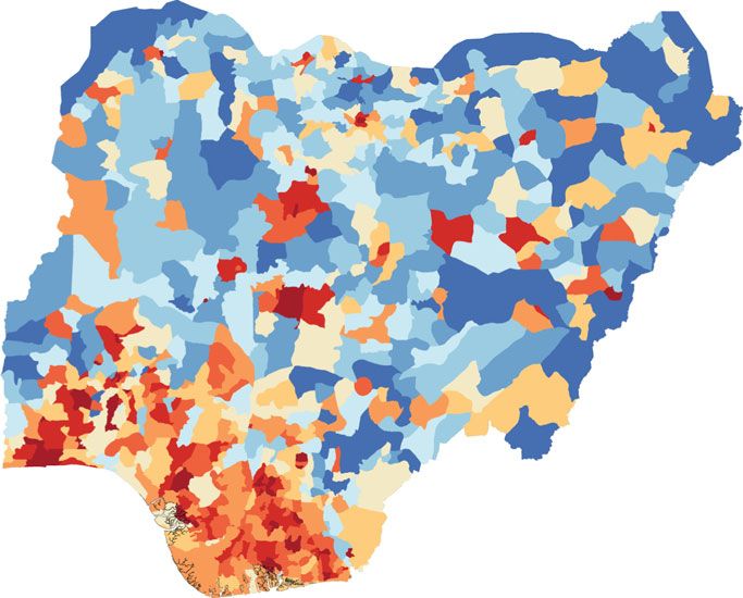
ARTICLE                                                                                                                    NATURE COMMUNICATIONS | https://doi.org/10.1038/s41467-020-16185-w

L
      ocal-level measurements of human well-being are important                                                                lights imagery can measure country-level economic performance
      for informing public service delivery and policy choices by                                                              over time7, and that high-resolution (500k households living in 19,669 villages across 23 countries in
two orders of magnitude less frequently than a household in the                                                                Africa, drawn from nationally representative Demographic and
United States (Fig. 1b). While not all households need to be                                                                   Health Surveys (DHS) conducted between the years 2009 and
observed to generate accurate economic estimates, sampling                                                                     2016 (Supplementary Fig. 1, Supplementary Table S1). We
enough households to generate frequent and reliable national-                                                                  focus on asset wealth rather than other welfare measurements
level statistics is alone likely to be expensive, requiring an esti-                                                           (e.g. consumption expenditure) as asset wealth is thought to be a
mated $1 billion USD annual investment in lower-income                                                                         less-noisy measure of households’ longer-run economic well-
countries to measure a range of indicators relevant to the Sus-                                                                being13,14, is a common component of multi-dimensional poverty
tainable Development Goals6. Expanding these efforts to generate                                                               measures used by development practitioners around the world, is
reliable estimates at the local level would add dramatically to                                                                actively used as a means to target social programs14,15, and is
these costs.                                                                                                                   much more widely observed in publicly available georeferenced
   Although existing data are scarce and traditional collection                                                                African survey data. Following standard approaches13,16, for each
methods expensive to scale, other potentially relevant data for the                                                            household we compute a wealth index from the first principal
measurement of well-being are being collected increasingly fre-                                                                component of survey responses to questions about ownership of
quently. For instance, while most African households are never                                                                 specific assets (“Methods”). We pool all households in our sample
observed in consumption or wealth surveys, their location                                                                      in the principal components estimation such that the derived
appears on average at least weekly in cloud-free imagery from                                                                  index is consistent over both space and time, and then average
multiple satellite-based sensors (Fig. 1b), and will have been                                                                 household values to the enumeration area level (also called
observed in multispectral imagery at least annually for more than                                                              clusters, and roughly equivalent to villages in rural areas or
a decade.                                                                                                                      neighborhoods in urban areas), the level at which geocoordinates
   Here we study whether such imagery can be used to accurately                                                                are available in the public survey data. This approach assumes
measure local-level well-being over both space and time in Africa.                                                             that assets contribute similarly to wealth across all countries in
Earlier work demonstrated that coarse (1 km/pixel) nighttime                                                                   our data. Alternative methods of constructing the index using

    a                                                       b
                                                                                                               1                                                                           PlanetScope (3m)
                                                            Avg. household revisit interval (days)

                                                                                                          a week                                                                           Sentinel 2 (10m)
                                                                                                                                                                                           LandSat 5-8 (30m)
                                                                                                         a month
                                                                                                            100                                                                            Digital Globe ( 10
               Never
                                                                                                                    2000    2002   2004   2006   2008 2010   2012   2014   2016     2018
                                                                                                                                                    Year

Fig. 1 Economic data from household surveys are infrequent in many African countries. a Frequency of nationally representative household
consumption expenditure or asset wealth surveys across Africa, 2000–2016. b Average household revisit rate for surveys and average location revisit rate
for various resolutions of satellite imagery over time. Survey revisit rate, the average time elapsed between observations of a given household in nationally
representative expenditure or wealth surveys, is calculated as number of total person-days (population × 365) divided by the number of person-days
observed in a given year. Satellite revisit rate estimates are calculated as the number of days in a year divided by the average number of images taken in a
year across 500 randomly sampled DHS clusters in African countries, only counting images with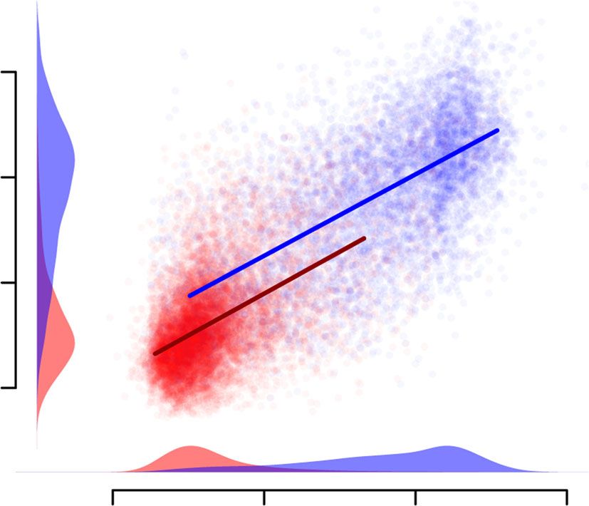
NATURE COMMUNICATIONS | https://doi.org/10.1038/s41467-020-16185-w                                                                  ARTICLE

only directly observable subsets of these assets, or which allow the            transfer learning approach8. Perhaps surprisingly, this trend
mapping of assets to the wealth index to differ by country and                  holds even for highly data-limited settings: even when trained on
year, yield very similar wealth estimates (Supplementary Fig. S2),              data from only 5% of the surveyed clusters (n < 1000), our best
and the wealth index is highly correlated with log consumption                  models trained end-to-end outperform transfer learning (Fig. 3c).
expenditure (weighted r2 = 0.5, Supplementary Fig. S3) in a small                  A nearest neighbor model that predicts wealth in a given
subset of countries where consumption data are available.                       location from wealth in locations with similar nightlights values
   We then train a convolutional neural network (CNN) to pre-                   performs nearly as well as the deep learning models in predicting
dict the village- and year-specific measure of wealth, using tem-                spatial variation, and much better than a linear model using scalar
porally and spatially matched multispectral daytime imagery                     nightlights as input (Fig. 3a, b)—although neither nightlights
from 30m/pixel Landsat and
ARTICLE                                                                                                                  NATURE COMMUNICATIONS | https://doi.org/10.1038/s41467-020-16185-w

                      a                                       Village level                                                    b                                        District level
                                                              r 2: 0.67, 0.70                                                                                           r 2: 0.75, 0.83; 0.67, 0.72
                                                                                                                                                                          Weighted; Unweighted

                                                         2                                                                                                         2

                         Survey-measured asset wealth

                                                                                                                                   Survey-measured asset wealth
                                                         1                                                                                                         1

                                                         0                                                                                                         0

                                                        –1                                                                                                        –1

                                                                  –1            0                 1             2                                                           –1            0                 1             2
                                                                             Satellite-predicted asset wealth                                                                          Satellite-predicted asset wealth

                      c                                                                                                        d
                                                                                                                          Mean r 2
                                                                                                                        0.50

                                                                                                                        0.60

                                                                                                                        0.70

                                                                                                                        0.75

                                                                                                                        0.80

                                                                                                                        0.85

                                                                                                                          1

                                                                                                                         NA

                      e                                                                                                        f
                                                             r 2: 0.82, 0.89; 0.73, 0.81                                                                               r 2: 0.71, 0.83; 0.54, 0.76
                                                               Weighted; Unweighted                                                                                      Weighted; Unweighted
                                                        2                                                                                                          2
                      Census-measured asset wealth

                                                                                                                               Census-measured asset wealth

                                                        1                                                                                                          1

                                                        0                                                                                                          0

                                                        –1                                                                                                        –1

                                                             –1                 0                 1                 2                                                  –1                0                  1                 2
                                                                            Survey-measured asset wealth                                                                              Satellite-predicted asset wealth

Fig. 2 Satellite-based predictions explain the majority of variation in survey-based wealth estimates in all countries, and validate well against
independent ground measures. a Predicted wealth index versus DHS survey-measured wealth index across all locations and survey years; each point is a
survey enumeration area (roughly, village) in a given survey-year, with satellite predictions generated by the CNN MS+NL model for each country from a
model trained outside that country (predictions from 5-fold cross validation). r2 values in red report goodness-of-fit on pooled observations, whereas
values in black are the average of r2 calculated within country-years. b As for a, but indices aggregated to the district level. c Average r2 over survey years
at the village level, by country. d Average r2 over survey years at the district level, by country. e Comparison of DHS-based to independent census-based
asset wealth at the district level, for available census measures within 4 years of DHS survey. f Comparison of asset wealth predicted by the CNN MS+NL
model in held-out-countries to the independent census-based asset measures at the district level. In b, e, and f, r2 is reported both weighted and
unweighted by the number of villages contributing to each district-level average. The number of villages is represented by the dot size.

4                  NATURE COMMUNICATIONS | (2020)11:2583 | https://doi.org/10.1038/s41467-020-16185-w | www.nature.com/naturecommunications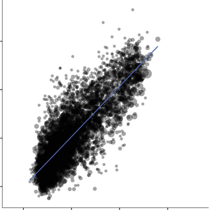
NATURE COMMUNICATIONS | https://doi.org/10.1038/s41467-020-16185-w ARTICLE
a 0.67 0.70 b 0.69 0.70 c
0.75
CNN MS + NL
0.66 0.70 0.68 0.7
CNN MS+NL
CNN NL 0.7
CNN NL
r 2 on held out countries
0.66 0.69 0.67 0.69
CNN MS
KNN scalar NL 0.65
0.62 0.65 0.66 0.67
CNN MS CNN transfer
0.6
0.56 0.6 0.59 0.59
CNN transfer
0.55
0.15 0.42 0.21 0.41
Linear scalar NL
0.5
0 0.2 0.4 0.6 0.8 0 0.2 0.4 0.6 0.8 0 0.2 0.4 0.6 0.8 1
r2 r2 % of data used in training
d e
0.7
2 CNN MS+NL
CNN NL
0.6
KNN
Observed wealth
r 2 on held out countries
1 0.5
CNN MS
0.4
CNN transfer
0 0.3
0.2 Linear scalar NL
–1 2
r = 0.40
r 2 = 0.32
0.1
0
–1 0 1 2 1 2 3 4 5 6 7 8 9 10
Predicted wealth Deciles of data used
Fig. 3 Performance by model and across different samples. a Predictive performance of satellite predictions trained using 5 different machine learning
models; NL nightlights, MS Landsat multispectral, and transfer transfer learning on nightlights with RGB Landsat imagery. Each grey line indicates the
performance (r2) on a held-out country-year, black lines and text show the average across country-years, and red lines and text show the r2 on the pooled
sample. b As in a but for evaluation on held-out villages within the same country. c Performance by amount of training data used. d Performance of CNN
MS+NL model in urban versus rural regions in held-out countries. Model is trained on all data in training set and then applied separately to either urban or
rural clusters in held-out countries. Each dot is an urban (blue) or rural (red) cluster, with densities showing the distribution of predicted (x-axis) and
ground-measured (y-axis) wealth index. e Performance across the wealth distribution. Experiments were run separately for increasing percentages of the
available clusters (e.g., x-axis value of 4 indicates that all clusters below 40th percentile in wealth were included in the test set).
patterns (Supplementary Fig. S10). Aggregating ground- and of the model’s explanatory power, at least in cross section,
satellite-based estimates to the district level again leads to appears to be in separating wealthier clusters from poorer clusters
substantial performance improvements (Fig. 4b), with predictions rather than in separating the poor from the near poor (Fig. 3d).
of asset wealth changes explaining up to 50% of the ground- Performance at the country level (as shown in Fig. 2c) is not
estimated changes in asset wealth. Improved performance with strongly related to country-level statistics on headcount poverty
aggregation is again consistent with errors cancelling when either rates, urbanization, agriculture, or income inequality (Supple-
the predictions or ground data are averaged. To our knowledge, mentary Fig. S11), although we do find that model performance is
these are the first known remote-sensing based estimates of local- somewhat worse in settings where within-village variation in
level changes in economic outcomes over time across a broad wealth is high. Poorer performance in these settings could be
developing country geography, and provide benchmarks for because our model has difficulty making accurate predictions in
future work. locally heterogeneous environments (a problem likely amplified
by the random noise that has been added to the data; see below),
Understanding model performance. While some of the com- or because sample-based estimates from the ground surveys are
bined model’s overall performance in spatial prediction derives themselves more likely to be noisy when local variation is high.
from distinguishing wealthier urban areas from poorer rural Other sources of noise in the ground data (e.g. due to survey
areas, the model is still able to distinguish variation in wealth recall bias, sampling variation or geographic inaccuracies) could
within either rural or urban areas (Fig. 3d). In either case, much also worsen model performance. To explore the overall role of
NATURE COMMUNICATIONS | (2020)11:2583 | https://doi.org/10.1038/s41467-020-16185-w | www.nature.com/naturecommunications 5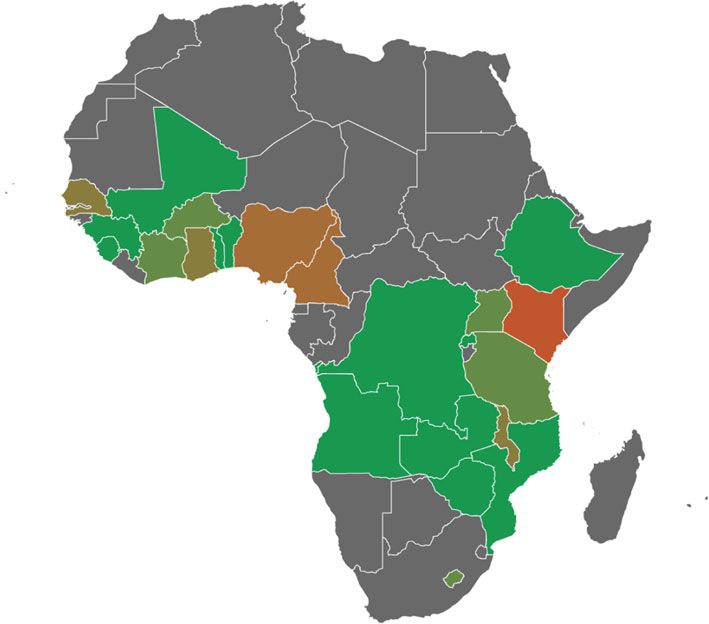
ARTICLE                                                                                               NATURE COMMUNICATIONS | https://doi.org/10.1038/s41467-020-16185-w

    a                                                                                                     b
                                        r 2 = 0.35                                                                                               r 2 = 0.51, 0.43

                                  2
                                                                                                                                      2
     LSMS index of differences

                                                                                                          LSMS index of differences
                                  0
                                                                                                                                      0

                                 –2

                                                                                                                                      –2

                                               –2                0                  2                                                             –2                 0                   2
                                                      MS Predicted index of differences                                                                    MS Predicted index of differences

    c                                                                                                     d
                                  0.0                0.1            0.2            0.3          0.4                                        0.0             0.1            0.2            0.3   0.4
                                                                    r2                                                                                                     r2
                                                                                                 NL                   MS                         MSNL

Fig. 4 Satellite predictions of ground-measured changes in wealth over time. a Performance of satellite-based model trained to predict the index of the
change in wealth over time at the village level. The index is computed by finding the changes in assets at a household level and creating an index of those
changes. Plot shows performance of model trained to predict this index of changes at the village level. b Same as a, but with observations aggregated to the
district level. Dot size represents number of village observations in each district, and r2 is reported both weighted (r2 = 0.51) and unweighted by number of
villages. c, d Cross-validated r2 of models trained on multispectral (MS, red), nightlights (NL, blue), and both (MSNL, green). Every reported r2 in c, d is
unweighted.

ground-based error in model performance, we take two                                                      suggests that locational noise in ground data is reducing model
approaches. First, we compare both model-based and ground-                                                performance by r2 = 0.07, or roughly the difference between our
based measures against an independent measure of asset wealth                                             best and worst performing CNN models (Fig. 3).
derived from census data in eight countries, with the comparison
made at the district level, the lowest level of geographic                                                Downstream tasks. To demonstrate the applicability of our
identification available in public census data. We find that                                                satellite-based estimates to downstream research or policy tasks,
ground-based measures are only slightly more correlated with this                                         we consider two use cases. The first is understanding why some
independent wealth measure than our model-based estimates,                                                locations are wealthier than others. Here we study associations
and both are highly correlated with the independent estimate                                              between wealth and exposure to extreme temperatures, as much
(Fig. 2e, f). This suggests that at least some of the prediction error                                    past work has indicated the wealth-temperature relationship is
in our main results derives from noise in the survey data.                                                nonlinear19,20, and because temperature data are readily avail-
    Second, a known source of error in our ground data is the                                             able for all study locations in an independent gridded dataset21.
random noise added to village-level geo-coordinates by the survey                                         Ground-based survey data indicate a non-linear relationship
implementers to protect privacy. In practice this jitter creates                                          between village-level wealth and maximum temperature in the
geographic misalignment between our input imagery and the true                                            warmest month, and out-of-country estimates from CNN-based
location of the surveyed villages; our approach is to look at all                                         models recover this relationship very closely (Fig. 5a, “Meth-
pixels in the 6.72 × 6.72 km neighborhood of the provided GPS                                             ods”); estimates from simple scalar nightlights models do not.
location assuming that the village’s true location falls in this                                          While none of these cross-sectional estimates are well suited for
neighborhood (6.72 km is the neighborhood defined by the input                                             causal identification of the impact of temperature on wealth19,22,
size of of our CNN architecture and the pixel size of our imagery;                                        we view the close match between satellite- and ground-based
see “Methods”), but much of this information might not be                                                 estimates of the temperature-wealth relationship as evidence
relevant to the specific village’s asset wealth. To understand the                                         that satellite-based estimates can be useful for these types of
performance cost of this noise, we iteratively add additional                                             research questions.
locational noise to our training data and then re-evaluate model                                             We also use our estimates to evaluate the hypothetical targeting
performance on test data which are either also additionally                                               of a social protection program (e.g. a cash transfer), in which all
jittered or not. Performance degrades with additional jitter                                              villages below some asset level receive the program and villages
(Supplementary Fig. S12), although much less rapidly when                                                 above the threshold do not. Targeting on survey-derived asset
evaluating on data that have not also been additionally jittered.                                         data is a common approach to program disbursement in
This suggests that the true (unobserved) performance of our main                                          developing countries23. We compare targeting accuracy, defined
results is higher than we report, given that we are evaluating on                                         as the percent of villages receiving the correct program, using
data that have been jittered. Using these results to extrapolate                                          estimates from different satellite-based models, under the
backward to a hypothetical setting of no jitter in training data                                          assumption that survey-based ground data describe the true asset

6                                            NATURE COMMUNICATIONS | (2020)11:2583 | https://doi.org/10.1038/s41467-020-16185-w | www.nature.com/naturecommunications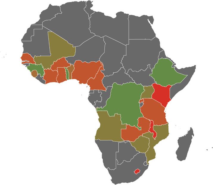
NATURE COMMUNICATIONS | https://doi.org/10.1038/s41467-020-16185-w ARTICLE
a b
Linear scalar NL 1.0
0.0
0.9
−0.2
Targeting accuracy
CNN transfer CNN MS+NL
Wealth index
KNN scalar NL
0.8
−0.4
CNN MS+NL
0.7 CNN transfer
−0.6 KNN scalar NL
0.6 Linear scalar NL
−0.8 Survey data
0.5
20 25 30 35 40 10th 20th 30th 40th 50th
Maximum temperature (°C) Targeting threshold (percentile)
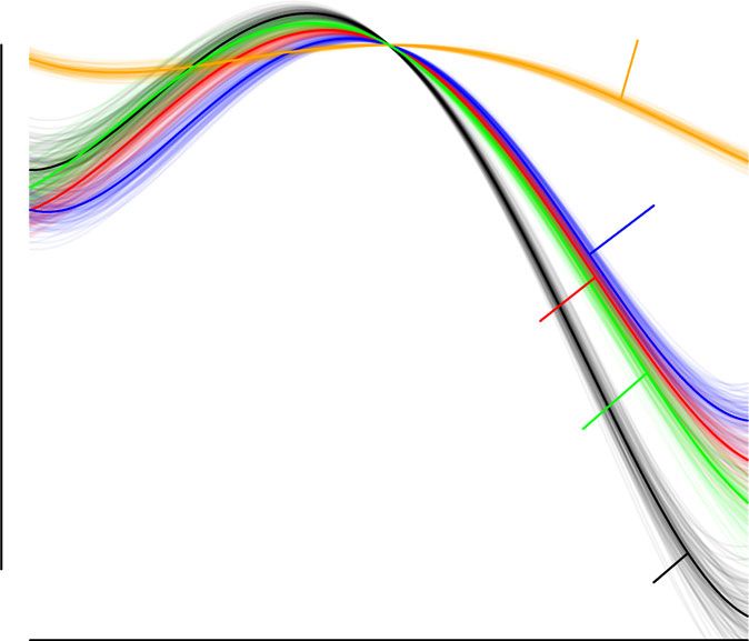
Fig. 5 Using satellite-based wealth predictions in downstream tasks. a Cross-sectional relationship between average maximum temperature and wealth
across survey locations, as estimated with survey wealth data (black) and estimates from three satellite-based models. Each line is a bootstrap of the
cross-sectional regression (100 bootstraps, sampling villages with replacement). Best-performing models recover temperature-wealth relationships that
are closest to estimates using ground-measured data, and CNN-based models perform much better than scalar nightlights models. b Evaluation of a
hypothetical targeting program in which all villages below some desired threshold in the asset distribution receive the program (e.g. a cash transfer) and
villages above the threshold do not. We compare targeting accuracy, defined as the percent of villages receiving the correct program, using estimates from
the same four satellite-based models as in a, under the assumption that survey-based ground data provide the true asset distribution. For instance, using
MS+NL estimates to allocate a program to households below median wealth yields a targeting accuracy of 81%, versus 75% for CNN Transfer and 62% for
scalar NL models. These estimates likely understate true targeting accuracy, given that ground data are themselves measured with some noise.
a b NL imagery c NL predictions h
d MS imagery e MS predictions
f Survey wealth g MS+NL predictions
Wealth index
–1.0 –0.5 0.0 0.5 1.0
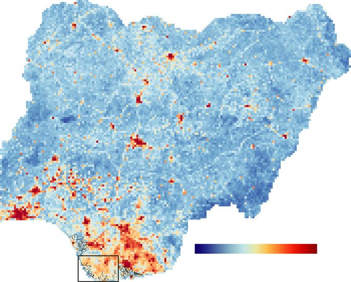
Fig. 6 Spatial extent of imagery allows wealth predictions at scale. a Satellite-based wealth estimates across Nigeria at pixel level. b, d Imagery inputs to
model over region in Southern Nigeria depicted in box in a. f Ground truth input to model over the same region. c, e, g Model predictions with just
nightlights (NL) as input, just multispectral (MS) imagery as input, and the concatenated NL and MS features as input. In this region, the model appears to
rely more heavily on MS than NL inputs, ignoring light blooms from gas flares visible in b. h Deciles of satellite-based wealth index across Nigeria,
population weighted using Global Human Settlement Layer population raster, and aggregated to Local Government Area level from the Database of Global
Administrative Areas.
distribution. Our best performing satellite models again perform not also associated with high wealth (Fig. 6b–g). Pixels are easily
well on this task (Fig. 5b). For instance, using MS+NL estimates aggregated to higher administrative units using existing popula-
to allocate a program to households below median wealth yields a tion rasters, and show strong latitudinal gradients of wealth
targeting accuracy of 81%, versus 75% for a CNN Transfer model across the country (Fig. 6h).
and 62% for a scalar nightlights model. Importantly, these Generating the pixel-level raster involves processing ~9.1 billion
estimates likely understate true targeting accuracy given that pixels of daytime and nighttime imagery. Once the pipeline is
ground data are themselves measured with some noise. developed, going from these raw imagery inputs to the prediction
raster takes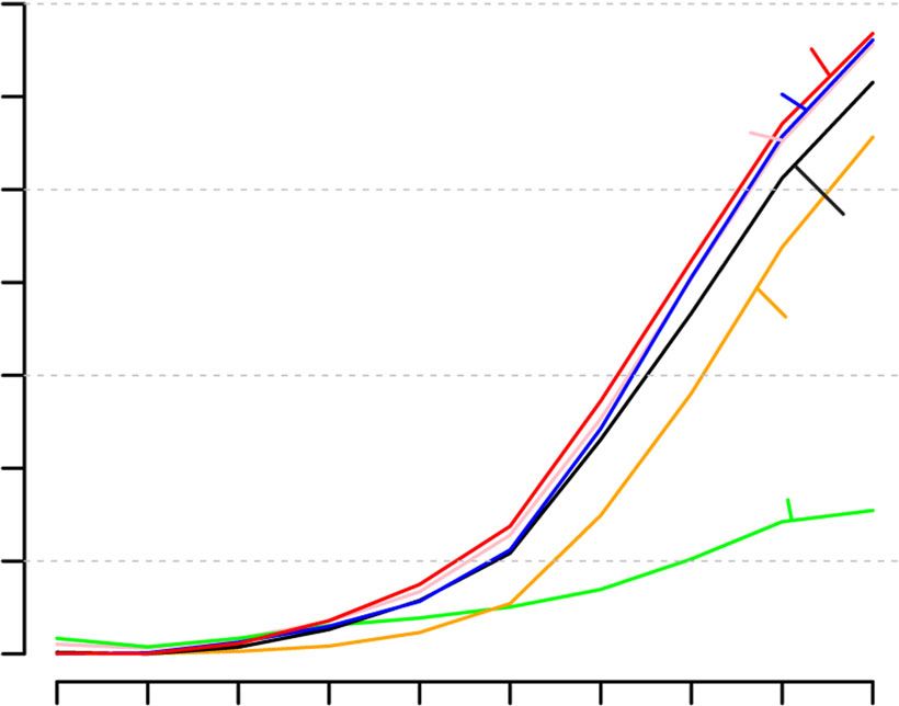
ARTICLE                                                                            NATURE COMMUNICATIONS | https://doi.org/10.1038/s41467-020-16185-w

Discussion                                                                              Replicating the wealth index in other contexts. We then create similar asset
Our satellite-based deep learning approach to measuring asset                           indices using two separate external data sets: census data from countries whose
                                                                                        censuses report asset ownership questions, and data from Living Standards Mea-
wealth is both accurate and scalable, and consistent performance on                     surement Study (LSMS) conducted by the World Bank. In the publicly available
held-out countries suggests that it could be used to generate wealth                    census data, a 10 percent sample of microdata geolocated to the second adminis-
estimates in countries where data are unavailable. Results suggest                      trative level (roughly, district or county) is available from each country. We focus
that such estimates could be used to help target social programs in                     on countries with public data who conducted censuses within 4 years of a DHS
data poor environments, as well as to understand the determinants                       survey in our main sample and which had gathered data on assets similar to what
                                                                                        was available in DHS. We found that 8 countries (Benin, Lesotho, Malawi, Rwanda,
of variation in well-being across the developing world.                                 Sierra Leone, Senegal, Tanzania, and Zambia) had all asset variables used in DHS
   However, while our CNN-based approach outperforms                                    excluding motorbike and rooms per person. (Using DHS data, we find that the
approaches to poverty prediction that use simpler features com-                         original index and an index constructed excluding these two variables had an r2 =
mon in the literature (e.g. scalar nightlights7), the information the                   0.99.) Our overall census sample yielded a total of 2,157,000 households observed
                                                                                        in 656 administrative areas across these eight countries.
CNN is using to make a prediction is less interpretable than these                          As census data are only georeferenced at second administrative levels, both
simpler approaches, perhaps inhibiting adoption by the policy                           DHS and census datasets are aggregated to the second-level administrative
community. A key avenue for future research is in improving the                         boundaries provided in the census data. Census data is aggregated using census
interpretability of deep learning models in this context, and in                        household weights to construct representative district averages. A raw average
                                                                                        across households is used to construct the corresponding DHS value; DHS and
developing approaches to navigate this apparent performance-                            LSMS data do not provide household weights that allow construction of sub-
interpretability tradeoff.                                                              nationally representative estimates.
   Our deep learning approach is also perhaps best viewed as a                              We utilized asset wealth data from LSMS panel surveys for five countries
way to amplify rather than replace ground-based survey efforts, as                      (Malawi, Nigeria, Tanzania, Ethiopia, and Uganda). Cluster-level GPS coordinates
                                                                                        are provided, with clusters in urban areas jittered up to 2 km and clusters in rural
local training data can often further improve model performance                         areas jittered up to 10 km. We are able to measure asset wealth for 9000 households
(Fig. 3b), and because other key livelihood outcomes often                              over time in the LSMS data (roughly two orders of magnitude less than DHS),
measured in surveys—such as how wealth is distributed within                            distributed over ~1400 clusters. As LSMS data follow households over time, we
households, or between households within villages—are more                              created a village-level panel using only households that existed in the first wave of
difficult to observe in imagery. Similarly, our approach could also                      interviews, removing any newly formed households or households that were not in
                                                                                        later surveys. Additionally, where available, households that reported in the second
be applied to the measurement of other key outcomes, including                          survey that they had lived in their current location for less time than had elapsed
consumption-based poverty metrics or other key livelihood                               since the first survey (i.e. migrant families) were removed. LSMS data were
indicators such as health outcomes. Performance in these related                        processed to try to match our DHS index as closely as possible, both by including
domains will depend both on the availability and quality of                             the same assets and by matching asset quality definitions as similarly as possible.
                                                                                        The fridge and motorbike variables were not available in the LSMS data and were
training data, which remains limited for key outcomes such as                           excluded from the LSMS wealth index. Using DHS data, we find that the original
consumption in most geographies. Finally, our approach could                            index and an index constructed excluding the fridge and motorbike variables were
likely be further improved by the incorporation of higher-                              highly correlated, with an r2 of 0.974. While we cannot directly compare DHS and
resolution optical and radar imagery now becoming available at                          LSMS indices at the village level, district level estimates from the two sources have
                                                                                        an r2 of 0.60.
near daily frequency (Fig. 1b), or in combination with data from                            While our asset data cannot be used to directly construct poverty estimates—
other passive sensors such as mobile phones17 or social media                           standard poverty measures are constructed from consumption expenditure data,
platforms24. All represent scalable opportunities to expand the                         which are not available in DHS surveys—household consumption aggregates are
accuracy and timeliness of data on key economic indicators in the                       available in a subset of the LSMS data just described. Across six surveys in three
                                                                                        countries, we find our constructed wealth index is fairly strongly correlated with log
developing world, and could accelerate progress towards mea-                            surveyed consumption at the village level, with a weighted r2 of 0.50 (Supplementary
suring and achieving global development goals.                                          Fig. S3). These results are consistent with findings that asset indices and consumption
                                                                                        metrics are typically very comparable14, and suggest that our approach to wealth
                                                                                        prediction could perhaps be useful for consumption prediction as well, particularly as
Methods                                                                                 additional consumption data become available to train deep learning models.
Construction of asset wealth index. The asset wealth index is constructed from
responses to the set of questions about asset ownership that are common across
DHS countries and waves: number of rooms occupied in a home, if the home has
electricity, the quality of house floors, water supply and toilet, and ownership of a    Satellite imagery. We obtained Landsat surface reflectance and nighttime lights
phone, radio, tv, car and motorbike. Variables such as floor type are converted from     (nightlights) images centered on each cluster location, using the Landsat archives
descriptions of the asset to a 1–5 score indicating the quality of the asset. We then   available on Google Earth Engine. We used 3-year median composite Landsat
construct an asset index at the household level from the first principal component of    surface reflectance images of the African continent captured by the Landsat 5,
these survey responses, a standard approach in development economics13,16. This         Landsat 7, and Landsat 8 satellites. We chose three 3-year periods for compositing:
index is meant to capture household asset ownership as a single dimension, rather       2009–11, 2012–14, and 2015–17. Each composite is created by taking the median of
than act as a direct measure of poverty. By construction, the index has a mean equal    each cloud free pixel available during that period of 3 years. The motivation for
to 0 and standard deviation of 1 across households. Supplementary Table S4 pro-         using three-year composites was two-fold. First, multi-year median compositing
vides derived loadings for the first principal component.                                has seen success in similar applications as a method to gather clear satellite ima-
    Survey data are derived from 43 Demographic and Health Surveys (DHS)                gery26, and even in 1-year compositing we continued to note the substantial
surveys conducted for 23 countries in Africa from 2009 to 2016 (Supplementary           influence of clouds in some regions, given imperfections in the cloud mask. Second,
Table S1). In addition to the asset data, each DHS survey contains latitude/            the outcome we are trying to predict (wealth) tends to evolve slowly over time, and
longitude coordinates for each survey enumeration area (or cluster) surveyed, each      we similarly wanted our inputs to not be distorted by seasonal or short-run var-
roughly equivalent to a village in rural areas and a neighborhood in urban areas.       iation. The images have a spatial resolution of 30 m/pixel with seven bands which
We removed clusters with invalid GPS coordinates and clusters for which we were         we refer to as the multispectral (MS) bands: RED, GREEN, BLUE, NIR (Near
unable to obtain satellite imagery, leaving us with 19,669 clusters. To protect the     Infrared), SWIR1 (Shortwave Infrared 1), SWIR2 (Shortwave Infrared 2), and
privacy of the surveyed households, DHS randomly displaces the GPS coordinates          TEMP1 (Thermal).
up to 2km for urban clusters and 10km for rural clusters25; this introduces a source        For comparability, we also created 3-year median composites for our nightlights
of noise in our training data.                                                          imagery. Because no single satellite captured nightlights for all of 2009–2016, we
                                                                                        used DMSP27 for the 2009–11 composite, and VIIRS28 for the 2012–14 and
                                                                                        2015–17 composites. DMSP nightlights have 30 arc-second/pixel resolution and
Validating the wealth index. The PCA-based index is quite robust to methods of          are unitless, whereas VIIRS nightlights have 15 arc-second/pixel resolution and
calculation as well as variables included in the index. We compare our cross-           units of nWcm−2sr−1. The images are resized using nearest-neighbor upsampling
country pooled PCA index to a measure that is the sum of all the assets owned, a        to cover the same spatial area as the Landsat images. Because of the resolution
PCA constructed from only objects that are owned (e.g. TV, radio) and not from          difference and the incompatibility of their units, we treat the DMSP and VIIRS
housing quality scores which are more subjective, and country-specific asset indices     nightlights as separate image bands in our models.
created from running the PCA on each country separately. As shown in Supple-                Both MS and NL images were processed in and exported from Google Earth
mentary Fig. S2, correlations between the pooled PCA index we use and these             Engine29 in 255 × 255 tiles, then center-cropped to 224 × 224, the input size of our
alternative variants range from r2 = 0.80 to r2 = 0.98.                                 CNN architecture, spanning 6.72 km on each side (30 m Landsat pixel size × 224

8                    NATURE COMMUNICATIONS | (2020)11:2583 | https://doi.org/10.1038/s41467-020-16185-w | www.nature.com/naturecommunications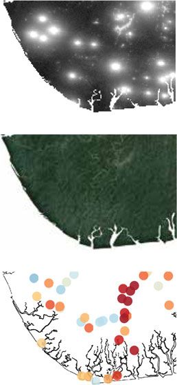
NATURE COMMUNICATIONS | https://doi.org/10.1038/s41467-020-16185-w                                                                                            ARTICLE

px = 6.72 km). Note that this means any survey cluster  pffiffiwhose
                                                           ffi     location coordinates      3-class classification problem. With these models trained to predict nightlights values
are artificially displaced by more than 4.75 km (6:72= 2) is completely beyond the          from daytime imagery, we froze the model weights and fine-tuned the final fully
spatial extent of the satellite imagery. Each band is normalized to have mean 0 and        connected layer to predict the wealth index. We note that our transfer learning
standard deviation 1 across our entire dataset. The raster of wealth in Nigeria in         experiments contain a much larger set of countries than the Jean et al.8 results, which
Fig. 5 was generated by exporting non-overlapping tiles from Google Earth Engine,          focused on five countries, and thus are not directly comparable.
following the same processing steps as for model training.
                                                                                           Baseline models. We train simpler k-nearest neighbor models (KNN) on night-
Deep learning models. Our deep CNN models use the ResNet-18 architecture (v2,              lights that predict wealth in a given location i as the average wealth over the k
with preactivation)30, chosen for its balance of compactness and high accuracy on          locations with nightlights values closest to that in i. In essence, this model allows a
the ImageNet image classification challenge31. We modify the first convolutional             non-linear and non-monotonic mapping of nightlights to wealth. The hyper-
layer to accommodate multi-band satellite images, and we modify the final layer to          parameter k is tuned by cross-validation. We also train a regularized linear
output a scalar for regression. For predicting changes in wealth and the “index of         regression on scalar nighlights (scalar NL) as a baseline model.
differences” on the LSMS data, we stack together the images from two different
years to create a 224 × 224 × (2C) image, where C is the number of channels in a           Training on limited data. To evaluate how models perform in even more data-
single satellite image.                                                                    limited situations, we trained our deep models on random subsets of 5%, 10%, 25%,
    The modifications to the first convolutional layer prevent direct initialization from    50%, and 100% of the full training data, repeated over 3 trials with different random
weights pre-trained on ImageNet. Instead, we adopt the same-scaled initialization          subsets. For each subset size, we report the mean r2 over the three trials (Fig. 3c).
procedure32: weights for the RGB channels are initialized to values pre-trained on
ImageNet, whereas weights for the non-RGB channels in the first convolutional layer
are initialized to the mean of the weights from the RGB channels. Then all of these        Data splits. For both DHS and LSMS survey data, we split the data into 5 folds of
weights are scaled by 3/C where C is the number of channels. The remaining layers of       roughly equal size for cross-validation. For the DHS out-of-country tests, we
the ResNet are initialized to their ImageNet values, and the weights for the final layer    manually split the 23 countries into the 5 folds such that each fold had roughly the
are initialized randomly from a standard normal distribution truncated at ±2. For the      same number of villages, ranging from 3909 to 3963 (Supplementary Table S2). As
models trained only on the nightlights bands, we initialized the first layer weights        described below, models were trained using cross-validation to select optimal
randomly using He initialization33. When predicting changes in wealth and when             hyperparameters. Each model was trained on 3-folds, validated on a 4th, and tested
predicting the index of differences on the LSMS data, we used random initialization        on a 5th. The fold splits used in the cross-validation procedure are shown in
instead, as it performed better than using same-scaled ImageNet initialization on the      Supplementary Table S3. For DHS in-country training, we split the 19,699 villages
validation sets (see “Cross-Validation”).                                                  into 5 folds such that there was no overlap in satellite images of the villages
    The ResNet-18 models are trained with the Adam optimizer34 and a mean                  between any fold, where overlap is defined as any area (however small) that is
squared-error loss function. The batch size is 64 and the learning rate is decayed by      present in both images. We used the DBSCAN algorithm to group together villages
a factor of 0.96 after each epoch. The models are trained for 150 epochs (200 epochs       with overlapping satellite images, sorted the groups by the number of villages per
for DHS out-of-country). The model with the highest r2 on the validation set across        group in decreasing order, then greedily assigned each group to the fold with the
all epochs is used as the final model for comparison. This is done as a regularization      fewest villages. We followed the same procedure to create 5 LSMS in-country folds.
technique, equivalent to early-stopping. We performed a grid search over the               We did not perform out-of-country tests with LSMS data.
learning rate (1e-2, 1e-3, 1e-4, 1e-5) and L2 weight regularization (1e-0, 1e-1, 1e-2,
1e-3) hyperparameters to find the model that performs the best on the validation
                                                                                           Cross-validation. For each of the input band combinations (MS, MS+NL, NL), we
fold. To prevent overfitting, the images are augmented by random horizontal and
                                                                                           trained five separate models, each with a different test fold. Of the four remaining
vertical flips. The non-nightlights bands are also subject to random adjustments to
                                                                                           folds, three folds were used to train the models, with the final fold designated as the
brightness (up to 0.5 standard deviation change) and contrast (up to 25% change).
                                                                                           validation set used for early stopping and tuning other hyperparameters (Supple-
Additionally, for predicting changes in wealth and the index of differences on the
                                                                                           mentary Table S3). Once the CNNs were trained, we fine-tuned the last fully
LSMS data, we randomize the order for stacking the satellite images (i.e. stacking the
                                                                                           connected layer using ridge regression with leave-one-group-out cross-validation.
before image on top of or below the after image), multiplying the label by −1
                                                                                           In the out-of-country setting, we fine-tuned the final layer individually for each test
whenever the after image was stacked on top to signify a reversed order.
                                                                                           country, using data from all other countries. Thus, the convolutional layers in the
    When using the two nightlights bands, we set pixels in the non-present band to
                                                                                           CNNs have effectively seen data from four of the 5-folds, while the final layer sees
all zeros. This ensures that the first-layer weights for that band are not updated
                                                                                           data from every country except the test country. In the in-country setting, we only
during back-propagation, because the gradient of the loss with respect to the
                                                                                           used data from the non-test folds for fine-tuning.
weights for the all-zero band becomes zero. Furthermore, since the ResNet-18
                                                                                               Ideally, the hyperparameters for machine learning models should be tuned by
architecture has a batch-normalization layer following each convolutional layer,
                                                                                           cross-validation for optimal generalization performance on unseen data. However,
there are no bias terms.
                                                                                           because training deep neural networks requires substantial computational
    For models incorporating both Landsat and nightlights (i.e. our combined
                                                                                           resources, leave-one-group-out cross-validation is prohibitively time intensive
model), we trained two ResNet-18 models separately on the Landsat bands and
                                                                                           (where in our setting, each group is a country). Consequently, we performed leave-
nightlights bands, respectively, and joined the models in their final fully connected
                                                                                           one-fold-out cross-validation for all the hyperparameters for the body of the CNN,
layer. In other words, we concatenated the final layers of the separate Landsat and
                                                                                           and only used leave-one-group-out cross-validation to tune the regularization
Nightlights models and trained a ridge-regression model on top. We found that
                                                                                           parameter for training the weights in the final fully connected layer.
this approach performed better than stacking the nightlights and Landsat bands
together in a single model.
    For DHS data, an average of 25.59 households (standard deviation = 5.59) were          Comparison with previous benchmarks. Our model achieves a cross-validated
surveyed for each village, compared to an average of 6.37 households (sd = 3.57) in        r2 = 0.67 on pooled cluster-level observations in held-out countries (or r2 = 0.70
LSMS. Due to the lower number of households surveyed for LSMS, which results in            when averaging over r2 values from each country). This meets or exceeds published
noisier estimates of village-level wealth, we weighted LSMS villages proportional to       performance on related tasks, including using high-resolution imagery and transfer
their surveyed household count in the loss function during training. We did not            learning to predict asset wealth in five African countries8 (r2 = 0.56), using call
weight DHS villages.                                                                       detail records to predict asset wealth in Rwanda17 (r2 = 0.62), and using survey data
                                                                                           and geospatial covariates to predict housing quality5 (r2 = 0.67), child stunting1
                                                                                           (r2 = 0.49), diarrheal incidence2 (r2 = 0.47 averaged over years) across sub-Saharan
Transfer learning models. We compared our end-to-end training procedure with
                                                                                           Africa or to predict standard of living in Senegal18 (r2 = 0.69). All values are for
the transfer learning approach first proposed by Jean et al.8. In this approach,
                                                                                           published cross-validated performance at the cluster or pixel level (except for
nightlights are a noisy but globally available proxy for economic activity (r2 ≈ 0.3
                                                                                           diarrheal incidence whose performance is only reported at the admin-2 level).
with asset wealth), and a model is trained to predict nighttime lights values from
                                                                                               As our primary focus is on constructing and evaluating out-of-country
daytime multispectral imagery. This process summarizes high-dimensional input
                                                                                           predictions, our results are not directly comparable to findings from other small
daytime satellite images as lower-dimensional feature vectors than can then be used
                                                                                           area estimate approaches that rely on having in-country surveys with which to
in a regularized regression to predict wealth.
                                                                                           extract covariates and make local-level predictions (e.g. refs. 35,36). However, our
    Because our images have a mixture of DMSP and VIIRS values, and the two
                                                                                           satellite-derived wealth estimates and/or the satellite-derived features themselves
satellites have different spatial resolutions, the binning approach in Jean et al.8 that
                                                                                           could be used as input to these small area estimates, and evaluating the utility of
treated nightlights prediction as a classification problem was unworkable. Instead, we
                                                                                           satellite-derived data in such settings is a promising avenue for future research.
framed transfer learning as a multitask regression problem. We extracted the neural
network’s final layer output predictions for both the DMSP value and the VIIRS value,
and regressed on whichever nightlights label was available for each daytime image. On      Research and policy experiments. To study whether our satellite-based estimates
the nightlights prediction task over locations sampled from all 23 DMSP countries,         can be used to shed light on the determinants of the spatial distribution of wealth—
our transfer learning models achieved performance of r2 = 0.82 when using RGB              a longstanding research question—we match our ground-based and satellite-based
bands and r2 = 0.90 when using all Landsat bands; these values are not directly            wealth estimates to gridded data on maximum temperature in the warmest
comparable to results in Jean et al.8, as that work posed nightlights prediction as a      month21. We study temperature as our potential wealth determinant because past

NATURE COMMUNICATIONS | (2020)11:2583 | https://doi.org/10.1038/s41467-020-16185-w | www.nature.com/naturecommunications                                                        9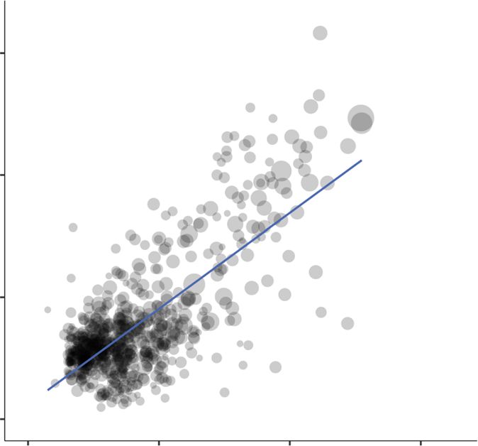
ARTICLE NATURE COMMUNICATIONS | https://doi.org/10.1038/s41467-020-16185-w
work has suggested that differences in temperature exert significant, non-linear 5. Tusting, L. S. et al. Mapping changes in housing in sub-Saharan Africa from
influence on economic output19,20, because temperature data are readily available 2000 to 2015. Nature 568, 391–394 (2019).
for all our study locations. 6. Espey, J. et al. Data for development: a needs assessment for SDG monitoring and
We extract the maximum average monthly temperature for each cluster in our statistical capacity development. Sustain. Dev. Solut. Netw. http://unsdsn.org/wp-
dataset (averaged over the years 1970–200021) and then flexibly regress wealth content/uploads/2015/04/Data-for-Development-Full-Report.pdf (2015).
estimates on temperature: 7. Henderson, J. V., Storeygard, A. & Weil, D. N. Measuring economic growth
wi ¼ f ðT i Þ þ εi ð1Þ from outer space. Am. Econ. Rev. 102, 994–1028 (2012).
8. Jean, N. et al. Combining satellite imagery and machine learning to predict
where wi is the wealth estimate for cluster i and f(Ti) is a fourth-order polynomial in poverty. Science 353, 790–794 (2016).
temperature. To capture uncertainty in our estimates of f(), we bootstrap Eq. (1) 100 9. Babenko, B. et al. Poverty mapping using convolutional neural networks
times for each different wealth measure, sampling villages with replacement. We trained on high and medium resolution satellite images, with an application in
compare estimates of f() when we measure wi using the ground data or when using Mexico. in Proc. NIPS 2017 Workshop on Machine Learning for the Developing
various satellite-based estimates: our benchmark MS + NL estimates, or the two World. https://arxiv.org/abs/1711.06323. (Neural Information Processing
main other published approaches, CNN transfer learning8 and scalar nightlights7. Systems Foundation, San Diego, CA, 2017).
Results are shown in Fig. 5a. We emphasize that these cross-sectional estimates of 10. Engstrom, R., Hersh, J. S. & Newhouse, D. L. Poverty from space: using high-
f() do not represent causal estimates of the impact of temperature on wealth, as resolution satellite imagery for estimating economic well-being. World Bank
many other factors are known to be correlated with both temperature and wealth Policy Res. Work. Pap. 1, 1–36 (2017).
(e.g. institutional quality, disease environment, nearby trading partners, etc.)22. 11. Head, A., Manguin, M., Tran, N. & Blumenstock, J. E. Can human
To study whether our satellite-based estimates can be used for policy tasks, we development be measured with satellite imagery? in Proc. Ninth International
evaluate the hypothetical targeting of a social protection program (e.g. a cash transfer),
Conference on Information and Communication Technologies and
in which all villages below some asset level receive the program and villages above that
Development, ICTD ’17, 8:1–8:11 (ACM, New York, 2017). https://dl.acm.org/
level do not. Such targeting on survey-derived asset data is a common approach to
citation.cfm?doid=3136560.3136576.
program disbursement in developing countries23. Because asset indices constitute a
12. Watmough, G. R. et al. Socioecologically informed use of remote sensing data
relative measure of wealth and it is not obvious how to set an absolute cut-off to
define who is poor, standard practice is instead to divide the population into to predict rural household poverty. Proc. Natl Acad. Sci. USA 116, 1213–1218
percentiles in the asset distribution and then designate bottom percentiles as poor15. (2019).
We follow that practice here. Using the ground data, we define a threshold wp;g 13. Sahn, D. E. & Stifel, D. Exploring alternative measures of welfare in the
absence of expenditure data. Rev. Income Wealth 49, 463–489 (2003).
corresponding to a chosen percentile p in the ground-measured asset distribution,
14. Filmer, D. & Scott, K. Assessing asset indices. Demography 49, 359–392 (2012).
and designate any village with wealth below that threshold as a program beneficiary
15. Alkire, S. et al. Multidimensional Poverty Measurement and Analysis (Oxford
(a treated village), i.e. t i;g;p ¼ 1½wi;g < wp;g , where wi,g is village i’s measured wealth
University Press, USA, 2015).
in the ground data and ti,g,p denotes that villages treatment status according to the 16. Filmer, D. & Pritchett, L. H. Estimating wealth effects without expenditure
ground data. We then follow the same procedure for a satellite-estimated wealth data-or tears: an application to educational enrollments in states of India.
distribution s, choosing the same percentile p in the satellite-estimated distribution
Demography 38, 115–132 (2001).
to define treatment. This yields each village’s treatment status under the satellite-
17. Blumenstock, J., Cadamuro, G. & On, R. Predicting poverty and wealth from
derived estimates t i;s;p ¼ 1½wi;s < wp;s . We note that we are fixing p between
mobile phone metadata. Science 350, 1073–1076 (2015).
ground- and satellite-based estimates rather than fixing the wealth threshold, such 18. Pokhriyal, N. & Jacques, D. C. Combining disparate data sources for improved
that the same overall number of villages are treated in both the ground-measured poverty prediction and mapping. Proc. Natl Acad. Sci. USA 114, E9783–E9792
case and the satellite-measured case. (2017).
Under the assumption that the ground-derived treatment statuses ti,g are
19. Burke, M., Hsiang, S. M. & Miguel, E. Global non-linear effect of temperature
correct, we then define targeting accuracy As,p as the proportion of satellite-
on economic production. Nature 527, 235 (2015).
derived treatment
P statuses that are correct under a given percentile cutoff p, i.e.
20. Nordhaus, W. D. Geography and macroeconomics: New data and new
As;p ¼ n1 ni¼1 1½t i;s;p ¼ t i;g;p , where n is the total number of villages. We compute
findings. Proc. Natl Acad. Sci. USA 103, 3510–3517 (2006).
As under different values of p ranging from the 10th to the 50th percentile, and for 21. Fick, S. E. & Hijmans, R. J. Worldclim 2: new 1-km spatial resolution climate
the same three different satellite-based wealth estimates s (MS+NL, transfer surfaces for global land areas. Int. J. Climatol. 37, 4302–4315 (2017).
learning, and scalar NL) used in Fig. 5. We emphasize that to the extent that the 22. Dell, M., Jones, B. F. & Olken, B. A. What do we learn from the weather? the
ground data wi,g are measured with noise, which we have strong evidence of (see
new climate-economy literature. J. Economic Lit. 52, 740–798 (2014).
Supplementary Fig. S12 and Fig. 2e, f), our estimated targeting accuracy likely
23. Grosh, M. E., DelNinno, C., Tesliuc, E. & Ouerghi, A. For Protection and
understates true targeting accuracy.
Promotion: The Design and Implementation of Effective Safety Nets (The
World Bank, 2008).
Reporting summary. Further information on research design is available in 24. Sheehan, E. et al. Predicting economic development using geolocated
the Nature Research Reporting Summary linked to this article. Wikipedia articles. In Proc. 25th ACM SIGKDD International Conference on
Knowledge Discovery & Data Mining, 2698–2706 (Association for Computing
Data availability Machinery, New York, NY, 2019).
Data to replicate all findings in the paper are available at https://github.com/sustainlab- 25. Burgert, C. R., Colston, J., Roy, T. & Zachary, B. Geographic displacement
group/africa_poverty. procedure and georeferenced data release policy for the Demographic and
Health Surveys. (ICF International, 2013). http://dhsprogram.com/pubs/pdf/
SAR7/SAR7.pdf.
Code availability 26. Azzari, G. & Lobell, D. B. Landsat-based classification in the cloud: an
Code to replicate all findings in the paper are available at https://github.com/sustainlab- opportunity for a paradigm shift in land cover monitoring. Remote Sens.
group/africa_poverty. Environ. 202, 1–11 (2017).
27. Hsu, F.-C., Baugh, K., Ghosh, T., Zhizhin, M. & Elvidge, C. DMSP-OLS
Received: 22 November 2019; Accepted: 8 April 2020; radiance calibrated nighttime lights time series with intercalibration. Remote
Sens. 7, 1855–1876 (2015).
28. Elvidge, C. D., Baugh, K., Zhizhin, M., Hsu, F. C. & Ghosh, T. Viirs night-time
lights. Int. J. Remote Sens. 38, 5860–5879 (2017).
29. Gorelick, N.et al. Google earth engine: Planetary-scale geospatial analysis for
everyone. in Remote Sensing of Environment (Elsevier, 2017). https://doi.org/
10.1016/j.rse.2017.06.031.
References 30. He, K., Zhang, X., Ren, S. & Sun, J. Identity Mappings in Deep Residual
1. Osgood-Zimmerman, A. et al. Mapping child growth failure in Africa between
Networks. in Computer Vision—ECCV 2016, (eds Leibe, B., Matas, J., Sebe, N.
2000 and 2015. Nature 555, 41 (2018).
& Welling, M.), 630–645 (Springer International Publishing, 2016). https://
2. Reiner, R. C. Jr et al. Variation in childhood diarrheal morbidity and mortality
doi.org/10.1007/978-3-319-46493-0_38https://arxiv.org/abs/1603.05027.
in Africa, 2000–2015. N. Engl. J. Med. 379, 1128–1138 (2018).
31. Russakovsky, O. et al. ImageNet large scale visual recognition challenge. Int. J.
3. Graetz, N. et al. Mapping local variation in educational attainment across
Computer Vis. 115, 211–252 (2015).
Africa. Nature 555, 48 (2018).
32. Perez, A. et al. Poverty prediction with public Landsat 7 satellite imagery and
4. Burke, M., Heft-Neal, S. & Bendavid, E. Sources of variation in under-5
machine learning. in Proc. NIPS 2017 Workshop on Machine Learning for the
mortality across sub-Saharan Africa: a spatial analysis. Lancet Glob. Health 4,
Developing World, (Long Beach, Neural Information Processing Systems
e936–e945 (2016).
Foundation, San Diego, CA, 2017). http://arxiv.org/abs/1711.03654.
10 NATURE COMMUNICATIONS | (2020)11:2583 | https://doi.org/10.1038/s41467-020-16185-w | www.nature.com/naturecommunicationsNATURE COMMUNICATIONS | https://doi.org/10.1038/s41467-020-16185-w ARTICLE
33. He, K., Zhang, X., Ren, S. & Sun, J. Delving deep into rectifiers: Surpassing human- Additional information
level performance on imagenet classification. In Proc. 2015 IEEE International Supplementary information is available for this paper at https://doi.org/10.1038/s41467-
Conference on Computer Vision (ICCV), ICCV ’15, 1026–1034 (IEEE Computer 020-16185-w.
Society, Washington, 2015). https://doi.org/10.1109/ICCV.2015.123.
34. Kingma, D. P. & Ba, J. Adam: A method for stochastic optimization. arXiv. Correspondence and requests for materials should be addressed to M.B.
Preprint at http://arxiv.org/abs/1412.6980 (2014).
35. Molina, I., Nandram, B. & Rao, J. et al. Small area estimation of general Peer review information Nature Communications thanks Gary Richard Watmough and
parameters with application to poverty indicators: a hierarchical bayes the other, anonymous, reviewer(s) for their contribution to the peer review of this work.
approach. Ann. Appl. Stat. 8, 852–885 (2014). Peer reviewer reports are available.
36. Elbers, C., Lanjouw, J. O. & Lanjouw, P. Micro-level estimation of poverty and
inequality. Econometrica 71, 355–364 (2003). Reprints and permission information is available at http://www.nature.com/reprints
Publisher’s note Springer Nature remains neutral with regard to jurisdictional claims in
Acknowledgements published maps and institutional affiliations.
We thank USAID Bureau for Food Security and the Stanford King Center on Global
Development for funding support. Ermon acknowledges National Science Foundation
grants #1651565 and #1522054 for additional support. Open Access This article is licensed under a Creative Commons
Attribution 4.0 International License, which permits use, sharing,
Author contributions adaptation, distribution and reproduction in any medium or format, as long as you give
M.B., S.E., and D.L. conceived of the study. G.A. and Z.T. processed and analyzed satellite appropriate credit to the original author(s) and the source, provide a link to the Creative
imagery. A.D. processed and analyzed survey and census data. C.Y. and A.P. trained deep Commons license, and indicate if changes were made. The images or other third party
learning models and analyzed their output with A.D. and M.B. C.Y., A.P., A.D., D.L., S.E., material in this article are included in the article’s Creative Commons license, unless
and M.B. interpreted results of model experiments. A.P. and C.Y. generated the wealth indicated otherwise in a credit line to the material. If material is not included in the
raster. C.Y., A.P., A.D., S.E., D.L., and M.B. wrote the paper. article’s Creative Commons license and your intended use is not permitted by statutory
regulation or exceeds the permitted use, you will need to obtain permission directly from
the copyright holder. To view a copy of this license, visit http://creativecommons.org/
Competing interests licenses/by/4.0/.
M.B., D.L., and S.E. are co-founders of AtlasAI, a company that uses machine learning to
measure economic outcomes in the developing world. A.P. and G.A. conducted the research
for this paper while students or employees at Stanford, but are also now employed at AtlasAI. © The Author(s) 2020
NATURE COMMUNICATIONS | (2020)11:2583 | https://doi.org/10.1038/s41467-020-16185-w | www.nature.com/naturecommunications 11You can also read