Topic modeling and bias analysis in a large scale spanish text dataset
←
→
Page content transcription
If your browser does not render page correctly, please read the page content below

Universitat Politècnica de Catalunya (UPC) - BarcelonaTech

       MASTER IN ARTIFICIAL INTELLIGENCE (MAI)

Topic modeling and bias analysis in a
  large scale spanish text dataset

            Facultat d’Informàtica de Barcelona (FIB)

                 Facultat de matemàtiques (UB)

           Escola tècnica superior d’ingenyeria (URV)

Author: Òscar Hernández Saborit
Advisor: Marta Ruiz Costa-jussà
Co-advisor: Quim Moré López

                         April 18, 2021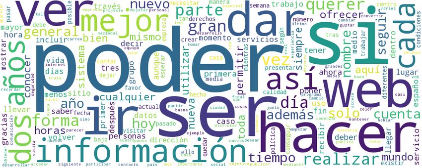
Abstract

In a world where data generation is doubled continuously, the ability to efficiently classify
and analyze large amounts of data is key to success. In this thesis, we will describe the
implementation of a distributed topic modelling pipeline and put it in practise against a
45TB dataset, demosntrating how HPC is essential to deal such quantity of data. We will
show the different problems that can arise when dealing with a huge amount of unsupervised
data and discuss the possible solutions. On the other hand, we will also play with word
embeddings, we will train different GloVe vectors to later compare them at different levels,
demonstrating how we can identify gender bias in trained embeddings and prove that
gender bias is present in all the data selected from the previous modelling task.

                                             1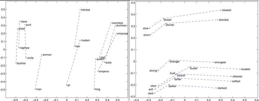
Contents

1 Introduction, motivation and goals                                                          1

2 State of the art                                                                            3
  2.1   Topic modelling . . . . . . . . . . . . . . . . . . . . . . . . . . . . . . . . .      3
  2.2   Word embeddings . . . . . . . . . . . . . . . . . . . . . . . . . . . . . . . .        4
        2.2.1   GloVe . . . . . . . . . . . . . . . . . . . . . . . . . . . . . . . . . .      5

3 Methodology                                                                                 6

4 Experimental work                                                                           8
  4.1   Supercomputing resources . . . . . . . . . . . . . . . . . . . . . . . . . . .         8
  4.2   The dataset . . . . . . . . . . . . . . . . . . . . . . . . . . . . . . . . . . .      9
        4.2.1   Size . . . . . . . . . . . . . . . . . . . . . . . . . . . . . . . . . . .     9
        4.2.2   Format . . . . . . . . . . . . . . . . . . . . . . . . . . . . . . . . . .    10
  4.3   Topic modelling experimentation . . . . . . . . . . . . . . . . . . . . . . .         10
        4.3.1   Preprocessing pipeline . . . . . . . . . . . . . . . . . . . . . . . . .      11
        4.3.2   Running LDA . . . . . . . . . . . . . . . . . . . . . . . . . . . . . .       15
        4.3.3   Topic modelling results and discussion . . . . . . . . . . . . . . . .        18
  4.4   Bias analysis . . . . . . . . . . . . . . . . . . . . . . . . . . . . . . . . . . .   22
        4.4.1   Data gathering pipeline . . . . . . . . . . . . . . . . . . . . . . . . .     22
        4.4.2   Bias analysis with glove . . . . . . . . . . . . . . . . . . . . . . . .      23
        4.4.3   Bias analysis results and discussion . . . . . . . . . . . . . . . . . .      25

5 Conclusions                                                                                 31

                                               2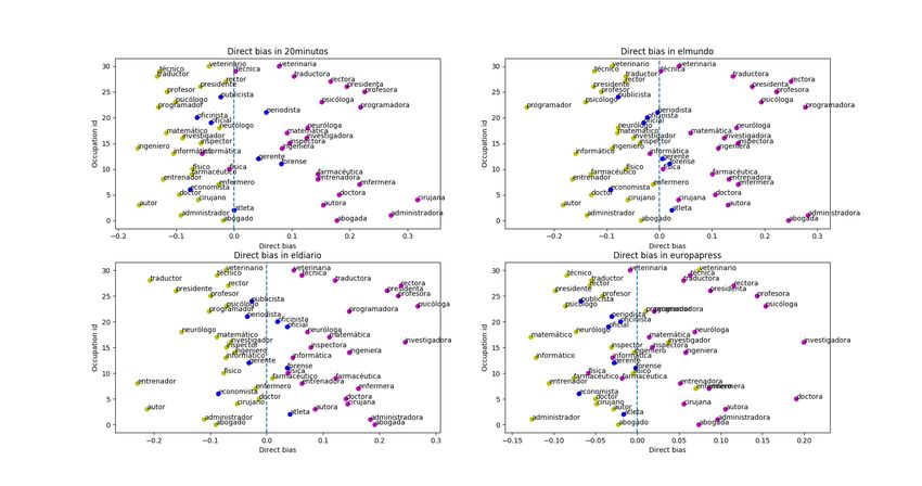
Contents                                                                                  3

Bibliography                                                                             33

A Word weghts for LDA models                                                             35
  A.1 Word weights for 10 topics . . . . . . . . . . . . . . . . . . . . . . . . . . .   35
  A.2 Word weights for 25 topics . . . . . . . . . . . . . . . . . . . . . . . . . . .   36

B Small datasets created                                                                 39
  B.1 Tested URL from different categories . . . . . . . . . . . . . . . . . . . . .     40
  B.2 Male-female-neutral occupations . . . . . . . . . . . . . . . . . . . . . . . .    42

List of Figures

 2.1   Document topic modelling example . . . . . . . . . . . . . . . . . . . . . .         3
 2.2   Vector relations from [5]. Man-woman left, comparative-superlative right. .          4
 2.3   Glove computation example from [5] . . . . . . . . . . . . . . . . . . . . .         5

 3.1   Block diagram for realized experiments . . . . . . . . . . . . . . . . . . . .       6

 4.1   Dataset size distribution across folders . . . . . . . . . . . . . . . . . . . .     9
 4.2   Parallel data processing pipeline . . . . . . . . . . . . . . . . . . . . . . . .   12
 4.3   Steps performed y worker nodes during parallel processing . . . . . . . . .         13
 4.4   Word cloud generated on the final data collected . . . . . . . . . . . . . . .      15
 4.5   Gathered data after the first parallel processing pipeline    . . . . . . . . . .   16
 4.6   Frequency distribution of the different words in the collected data . . . . .       16
 4.7   Word distribution across domains . . . . . . . . . . . . . . . . . . . . . . .      17
 4.8   Word cloud generated on the data after filtering . . . . . . . . . . . . . . .      18
 4.9   Coherence score among different topic number. (the lower, the better) . . .         18
 4.10 Webpage distribution across 10 topics . . . . . . . . . . . . . . . . . . . . .      19
 4.11 Webpage distribution across 25 topics . . . . . . . . . . . . . . . . . . . . .      20
 4.12 confusion matrix for web classification . . . . . . . . . . . . . . . . . . . .      20
 4.13 Selected news domains . . . . . . . . . . . . . . . . . . . . . . . . . . . . .      23
 4.14 Data cleaning pipeline for the news dataset . . . . . . . . . . . . . . . . . .      23
 4.15 Bias comparison with regard to model dimensionality . . . . . . . . . . . .          26
 4.16 Bias representation of the word in the él-ella vector . . . . . . . . . . . . .      27
 4.17 All models direct gender bias . . . . . . . . . . . . . . . . . . . . . . . . .      28
 4.18 Correlation between elmundo and eldiaro word gender biases . . . . . . . .           28

                                             4
List of Figures                                                                             5

   4.19 20minutos indirect gender bias words representation, baloncesto on the left,
        danza on the right . . . . . . . . . . . . . . . . . . . . . . . . . . . . . . .    29
   4.20 Political terms closer to PP (right-hand side) and to PSOE (left-hand side),
        20minutos dataset . . . . . . . . . . . . . . . . . . . . . . . . . . . . . . . .   30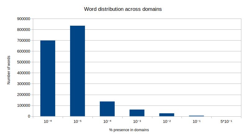
List of Tables

 4.1   Topic modelling objective . . . . . . . . . . . . . . . . . . . . . . . . . . .    11
 4.2   Pipeline implementations differences in collected data . . . . . . . . . . . .     14
 4.3   Different trained glove models . . . . . . . . . . . . . . . . . . . . . . . . .   24
 4.4   Direct gender bias computed on the male-female occupations list of words .         25

                                            6
Chapter 1
Introduction, motivation and goals
Every day, and consistently for the last years, an increasing amount of information is shared
worldwide on the internet. Comprehensive data of the world and its past/current/future
events and knowledge is stored everyday in the form of written data.
In late 90’s, Larry Page and Sergey Brin, successfully understood the potential of under-
standing this data, leading them to the foundation of one of the most relevant companies
around the world, Google Inc. Having web query and content understanding as their main
income source, companies like Google have pushed the technology forward, taking advan-
tage of hardware generational leaps to implement more computing intensive workloads,
materializing today’s deep learning frameworks like Tensorflow or Torch, allowing for the
creation of state of the art language processing models such as BERT.
NLP, what is commonly known as the collection of software developed to allow machines
to understand (and properly encode) human language, has existed on its own as a re-
search field for longer than these companies. However, original rule-based NLP systems
were starting to reach their limits, and during the last decade, NLP community has been
focused on new neural based solutions, as it can be appreciated in solution submissions to
NLP contests like semeval[1] .
Encouraged by this glowing ecosystem. I decided to test my skills and all the available
knowledge to develop the experiments reported in this thesis. Having an enormous dataset
available, the objective was to test different techniques to classify the enormous amount of
web crawled data. Trying to understand how companies like google process, classify and
extract information for their later use.
This project has 2 main goals. 1 - Develop a preprocessing and classification approach
1Introduction, motivation and goals 2 for a 45TB dataset of unannotated web-crawled data from spanish domains. 2 - Further analyse some of this data using state of the art techniques, identifying the underlying bias. The development of this work contributes in the exploration of new techniques for analyzing massive-sized datasets in an extremely parallel system, all without the use of any big data framework such as Spark or Hadoop. Additionally, current bias analysis techniques have been explored and used to evaluate raw data directly extracted from the classified, but barely processed dataset.
Chapter 2

State of the art

2.1     Topic modelling
Topic modelling techniques consist in different procedures that allow, with the use of a
variety of information, classify a collection of given sentences or documents into groups.
The idea is to group together those documents that share properties, and to do it in an
unsupervised manner.

                     Figure 2.1: Document topic modelling example

There are different techniques and approaches to develop this task. But nearly all of them
use at some point a statistical generative model, which allow to automatically define topics
based on word observations, and later classify each document based on the probabilities
of each one of its words to belong to a given topic. In the development of this project, I
have opted for the use of LDA[2](Latent Dirichlet Allocation), a generative discriminative

                                             3
2.2. Word embeddings 4 apporach that uses the Dirichlet statistical distribution to generate the words-topics affinity. Recent literature suggests to use LDA in combiantion with word-embeddings [3], as the relations encoded in those help LDA to better identify bonds between words. However, in my experiments, these variants have not been proposed, I have opted for a direct LDA approach. The main reasons behind this decision are: 1. Data requirements: LDA does not need the original sentences, word order does not matter and we are only interested in BoW, which is ideal to simplify an enormous corpus. This also allows me to prepossess data in a distributed way. 2. Time saving: Due to the quantity of the data, applying heavy preprocessing would simply take too much time. I am aiming for a simpler approach. 2.2 Word embeddings Word embeddings is the general term used for the representation of words in the NLP world. The idea behind them is that, instead of using a words as simple ids, which just work as identifiers and are not able to encode any kind of relationship between them, we use precomputed vector representations of the words. These vector representations of the words, which can be of different dimensionality, allow us to compute different relations between words. Via the use of arithmetical operations in the vectorial space, we are able to identify words that are similar in meaning (synonyms) or completely opposite (antonyms), concepts and words related with them...we are able to process words as meaningful data, and not just ids. As stated in Tomas Mikolov et al. [4], these was the necessary leap towards the creation of more capable and complex NLP mod- els. Nowadays, word embeddings are extensively (and almost indispensable) when dealing with natural language tasks. Figure 2.2: Vector relations from [5]. Man-woman left, comparative-superlative right.
2.2. Word embeddings                                                                        5

Although word embeddings need to be previously trained, they are portable. So, once a
model is trained, it can be used in different NLP tasks - if they share language -, though for
some specific tasks, it is also recommended to train embeddings on domain-specific corpus.
There are multiple alternatives for training word embeddings, being all formed by different
neural network topologies, the most relevant ones are word2vec [4] - with the CBOW and
the Skip-gram models -, and GloVe [5], which generally outperforms the former models
and has been the chosen one for the reported experiments.

2.2.1    GloVe
GloVe stands for gloval vector representations, and the main difference between other
local models like word2vec, is precisely that, the use of a Global occurrence matrix in
combination with local co-ocurrences. It is built by computing the similarity between
triplets of words, following the expression F(i,j,k) = P_ik/P_jk, where i,j,k are the
compared words and P_ik = X_ik/X_i, with X_ik being the number of times i and
k appear together, and X_i the number of times i appeared in the corpus. An example
can be appreciated in 2.3.

                     Figure 2.3: Glove computation example from [5]

Following this example, we see how when k is most similar to i, than to j, we get >1 values
(solid). When the opposite happens, we get
Chapter 3
Methodology
The development of the project has been structured in 3 different blocks. Starting from
a more general perspective, the first block consists in analyzing and understanding the
dataset. The second and third blocks aim for more specific tasks. The former is to prove
that the initial hypothesis of web domains being classified by its content with the use of
BoW is plausible, and the latter, evaluating the gender bias present in some of the data
collected, more specifically, news media. The schema in figure 3.1 show the different steps
that have been followed.
Figure 3.1: Block diagram for realized experiments
1. Dataset Exploration: The first part of the experiments consists in analyzing the
different characteristics of the available dataset. Files distribution, availability and
format are analyzed in order to evaluate the most adequate techniques for achieving
6Methodology 7
our objectives. Additionally, random samples of data are collected, to evaluate pos-
sible encoding problems, that will need to be corrected in the following steps.
2. Topic modelling: The second part of the experiments is the denser one. An MPI
code is built to preprocess the dataset and different alternatives for preprocessing are
evaluated. Issues with the different generated BoWs are discussed and the best is
used to feed different LDA models. U_mass score is used to evaluate the best num-
ber of topics for the LDA classification. Finally, a custom build small dataset is used
to validate some of the classification, and guess the content behind generated topics.
Final classification results are evaluated and possible alternatives are discussed.
3. Bias analysis: The third and last part of the experiments consists in a more in depth
analysis of some particular part of the dataset, the news webpages. The previously
used pipeline is modified, this time to gather the full corpus of selected URLs of the
dataset. A new preprocessing pipeline is deveoped to tokenize sentences and remove
sentence repetition. Different GloVe models are built and evaluated. Finally gender
bias is studied by using a male/female/neutral dataset of professional occupations
and results are discussed.Chapter 4
Experimental work
Following the aforementioned schema. The experiments will be divided in 3 parts: 1.
Dataset analysis, 2. Topic modelling approaches and finally 3. Bias analysis. But first, we
will introduce the supercomputing resources we have used to carry out the experiments
4.1 Supercomputing resources
We would not have been able to process such amount of data without supercomputing
resources provided by the Barcelona Supercomputing Center(BSC)[7]. First, they have
provided enough storage capacity to handle the 45TB dataset -plus all the extra data
collected in the experiments- via a distributed parallel filesystem(GPFS). Secondly, access
to 2 different architecture machines was also granted: Marenostrum4 and CTE-Power9.
GPFS: Known as general parallel filesystem. With approximately 15PB of storage
capacity, this shared filesystem allows the computing nodes of all machines in the
center share data on disk, extremely useful to avoid setting more complex big data
frameworks such as Hadoop or Spark.
Marenostrum4: General purpose cluster (NO-GPU). Formed by 3456 nodes, each
containing 48cpus and up to 380G of RAM.[8]
CTE-Power9: GPU cluster. Formed by 50 nodes, each containing 160cpus and 4
nvidia V100 acceletors (specially designed for AI pipelines), up to 580G of available
RAM.[9]
84.2. The dataset 9
4.2 The dataset
Extracting useful information of this dataset has been the main objective of the project.
So we should fairly devote some time to analyze its size, form and content.
It has been generated as a result of a massive crawling done by the BNE (biblioteca na-
cional de España)[10]. A crawling with the intention of recording each one of the .es
domain websites, in order to have a snapshot of the available information contained by
the websites aimed at the spanish people. We do not have more details on the crawling
implementation, but we will share our findings after some simple data exploration.
4.2.1 Size
The dataset contains a total of 507689 files. Ranging from sizes of 1MB to several GBs.
All these files are spread in different directories, with no apparent relation whatsoever.
In figure 4.1 we can appreciate this uneven data distribution by observing the difference
in size of the different data folders, containing as average 500GB of data, but with some
folders containing up to 3.7TB of data.
Figure 4.1: Dataset size distribution across folders
The total size of the dataset is around 45TB. Making clear that trying to process all these4.3. Topic modelling experimentation 10 data is the first challenge we will try to overcome. 4.2.2 Format With regard to the form of the data. As mentioned before, it is spread in the form of 507689 json files. The json data contains the following keys: url: Full URL where the info has been extracted from p: Text (and also HTML directives) contained in the URL heads: Headers or links of the given webpage (not always present) keywords: Keywords set to identify the web (not always present) The 2 keys of interest for this work are 1. url and 2. p. They contain the webpage in- spected, as well as the textual content we will aim to use for the analysis. As we will later showcase, data contained in “p” comes in a really dirty state, and several preprocessing will be needed to start getting a clean corpus. Regarding the file organization, there is none. Each json file may contain data for a single, or multiple URLs. Furthermore, the same url or data can be at the same time in multiple json files. 4.3 Topic modelling experimentation Our first objective was to extract relevant information from the files, and use that infor- mation to classify each one of the domains present in the data. The ideal result after this step would imply having a list of all domains present in the dataset, classified in their cor- responding area (news, sports, shop, company, blog...), as it can be appreciated in table 4.1. The complexity of this task, thought, remained in the quantity and quality of the data available. As shown in section 4.2, the quality is poor, and the quantity is overwhelming. So, the first step was to create a code thought for a large scale system (specifically Marenos- trum4), which was able to process the available data in a timely and distributed manner. Literature led me to prepare the data to run LDA (Latent Dirichlet Allocation)[2], as it would allow me to reduce the initial data by only storing a bag of words (BoW) for each one of the analysed domains, reducing significantly the size of the initial dataset (45TB).
4.3. Topic modelling experimentation                                                   11

                      Web domain                Topic (Class)
                      https://elperiodico.es            News
                      https://mundodeportivo.es        Sports
                      https://decathlon.es               shop
                      ...                                  ...

                          Table 4.1: Topic modelling objective

4.3.1    Preprocessing pipeline

With half a million files, trying to process all the data using a simple thread could have
taken months. As presented in the previous section 4.2.1, we are dealing with dense files,
which are unevenly distributed in the different folders that form our dataset. Even run-
ning in a full Marenostrum4 node could take weeks, so it was clear some multi node MPI
implementation was needed.
4.3. Topic modelling experimentation 12
Figure 4.2: Parallel data processing pipeline
Figure 4.2 shows the final structure of the implemented code. We can appreciate how the
master orchestrates the file distribution to the workers, which are continuously processing
data until the end of the pipeline, when all data is dumped to disk. Additionally, we can
observe how the pipeline has been built with a fault tolerant approach, as it is continuously
storing the processed data as breakpoints to avoid losing all the progress in case of failure.4.3. Topic modelling experimentation 13
Figure 4.3: Steps performed y worker nodes during parallel processing
Now focusing in the file preprocessing pipeline, we can appreciate in figure 4.3 the differ-
ent steps performed in order to clean and organize the data: 1.The first step is to extract the
root url, most of the dataset urls are of the form of https://elperiodico.es/news/new0001.html,
as we want to classify pure domains, such as elperiodico.es, we use regex rules to extract the
relevant part of the text. 2. data is not clean (contains several html tags and symbols), we
also use an HTML library to extract clean text 3. We will center in analyzing only spanish
text, so we filter all the data that is not correctly identified as spanish. 4 We tokenize the
text and remove all stopwords. 5. We finally count the number of appearances of each
token, and add it to their corresponding web domain.
Three different approaches were considered for carrying out this task.
2. First implementation: This first pipeline implementation ran as expected. We
3.
1.
submitted a Marenostrum job requesting for 10 nodes (480 tasks), a single master
task was able to handle correctly the 479 tasks of the workers preprocessing the data.
The job took approximately 2 days.
However, data generated was not good enough for running LDA. As it can be ap-
preciated in table 4.2, for the first preprocessing pipeline, the vocabulary size of this
first run was more than 189 million words. That exposed some issues: 1- Too big
vocabulary size to be handled in a timely manner (also considering memory restric-
tions). 2- Huge amount of words for the Spanish language.4.3. Topic modelling experimentation 14
A deep inspection of the gathered data, also revealed a couple problems that needed
to be addressed. 1- The data was not clean enough, my pipeline was still letting
through several non-spanish words, which increased my vocabulary size without pro-
viding useful information for the context of study. 2- There was a problem with the
dataset. Some of the text was wrongly stored, joining the end of some sentences with
the start of new ones. That resulted in a lot of fake compound words added to the
vocabulary.
2. Second implementation: After acknowledging the first try flaws, we decided to
correct them by adding slight modifications to the initial pipeline. For this second
try, we tried to correct the size of the vocabulary by implementing 2 extra processes
to the pipeline:
(a) Word stemming: With the purpose of taking generalizing words, we took the
approach of extracting the root sense of each word. In a traditional pipeline,
we would have gone for lemmatization as it would have provided accurate re-
sults. However, None of the lemmatization solutions were fast/good enough to
be processed in the pipeline.
(b) Only repeating words count: Apart from stemming, to solve the fake com-
pound words problem mentioned, we opted for just taking the words that ap-
peared more than 10 times in a given domain. This way we would be discarding
all those fake words that were randomly appearing in the dataset.
1. raw data 2. Stemming+ rep. 3. Dict. filtering
Dictionary words 189709389 3205200 1763567
Dictionary size 5300MB 73MB 42MB
Data collected 52000MB 2500MB 5800MB
Table 4.2: Pipeline implementations differences in collected data
As it can be observed in table 4.2, after these new additions to the pipeline, data
collection was significantly reduced. Data was more affordable to run LDA, however,
the word repetition was far from optimal. Data collected from each domain was
heavily reduced, as we were only keeping repeated words, and we were still dealing
with foreign language terms.4.3. Topic modelling experimentation 15
3. Final implementation: Finally, in order to address all the flaws mentioned earlier,
a definitive approach was taken. Given the bad quality of the data, we opted for
building a dictionary of valid words in spanish, and just work with the words that
appeared in it.
As we did not find any reliable compiled dictionary with all the spanish corpus. I
decided to build one myself. I developed a Crawling code to look for words in the
Spanish Real Academy Website[11]. The dictionary contains all the gathered RAE
words, and it is able to map each spanish verbal form to the infinitive. To cope with
plural words, we also added some versatility to the dict, allowing for variable letters
at the end of each word, which also had a reduced risk of introducing unknown words
In table 4.2, we can appreciate how the dict length of this new approach was smaller,
as I was avoiding all the non-spanish words. On the other hand, it can be appre-
ciated how the size of the extracted Corpus is greater than the previous approach,
as we removed the word repetition limitation. In figure 4.4 words are represented
proportionally to their frequency.
With that data collected, we were ready to start experimenting with LDA and the
topic modelling task.
Figure 4.4: Word cloud generated on the final data collected
4.3.2 Running LDA
Before running the algorithm, we decided to inspect the main features and understand the
collected dataset. Extracting topics with random information collected from web pages
would not be an easy task, and knowing about the dataset would help me better work with4.3. Topic modelling experimentation 16
the data.
Figure 4.5: Gathered data after the first parallel processing pipeline
Figure 4.5 represents the collected data, we can appreciate how each domain is represented
by the words that appear in it, also storing the number of times each word is repeated
into it. If we take a look at figure 4.6, frequency distribution of the collected data, we can
appreciate how half of the words appear less than 10 times, a fact that is already telling
us that most of the words will not be decisive for topic modelling.
Figure 4.6: Frequency distribution of the different words in the collected data4.3. Topic modelling experimentation 17
Further analyzing the collected dataset, in figure 4.7 we can appreciate the word distribu-
tion across domains. As expected, little words appear in more than 10% of the domains,
being these words not much informative (such as página, encontrar, nombre, mostrar, web,
poder. . . )
Figure 4.7: Word distribution across domains
After analyzing the collected data, different versions of the LDA algorithm were submitted,
playing with different filtering to make the data fit into the Power9 node memory (580G),
as well as with the objective of obtaining useful results.
We used the LDA implementation from the gensim[12] python package, which also comes
with a coherence evaluation method that was already used to evaluate the quality of the
topics. After several failed attempts, and based in previous figures 4.7 and 4.6, we ended
up filtering my BoW to contain words that fulfilled the following conditions: 1. Appear in
less than 20% and more than 0.1% of the documents. 2. Has at least 100 occurrences in the
full corpus. Resulting corpus after the clearance contained a vocabulary of 32223 words,
2% of the total 1763567. Remaining words can be appreciated in figure 4.8, if compared
to the initial wordcloud in 4.4, we can appreciate how most common and uninformative
words like poder, hacer, web, si... have been removed from the corpus.
Additionally, we also decided to center in the domains with a vocabulary size of, at least,
50 words. Cleaning from the corpus all those domains without enough information to be
relevant for the topic modelling. After removing these domains, total number of domains4.3. Topic modelling experimentation 18
was reduced from 4737799 to 1362194 (28%).
Figure 4.8: Word cloud generated on the data after filtering
4.3.3 Topic modelling results and discussion
Having filtered the data, we had to guess the correct number of topics to request to the
algorithm. As we had no idea on what to expect, we led the data guide me through this
decision. Using the u_masstopic coherence algorithm as score - it was implemented in
gensim, and found interesting literature about it[13] - we run the LDA requesting from 5
to 55 topics. Being the lower score the better for the coherence values, figure 4.9 clearly
shows 25 as the best number.
Figure 4.9: Coherence score among different topic number. (the lower, the better)4.3. Topic modelling experimentation 19
Another interesting way of judging the clustering, is by analyzing the most weighted words
in each one of the topics. In the annex files A.1 and A.2, word weights for the 10 and 25
topic execution are shown. By taking a quick look into it, the first thing that draws the
attention is the low weight each one of the words represent - something expected due to
huge diversity of content web pages may show -. But taking a closer look, we can identify
words that may infer to the main content of the web-page. We can see together words like
jugar", "club", "partido", "temporada" that are clearly referring to sports-related content,
as well as producto", "mas", "diseño", "venta", "compra" that could clearly refer to web-
portals specialized in selling stuff.
Further analyzing the 25 and 10 topic models, we filter each one of the 1362194 web-pages,
to evaluate how are they distributed across different topics, see figures 4.11 and 4.10. It
can be appreciated how they follow a similar pattern - webpages with no clear topic are
assigned to topic 0 -, in which there is a huge majority with no clear topic, but the other
ones are fairly distributed across other available topics.
Figure 4.10: Webpage distribution across 10 topics4.3. Topic modelling experimentation 20
Figure 4.11: Webpage distribution across 25 topics
As there is no annotated dataset to test our classification. We decided to build my own test
one, by using known webpages from which we know their content, and that we considered
should share topic. As we have special interest in press articles, we decided to check if the
classification was able to correctly distinguish between sports press and general press,a part
from that, we also added some extra webs that we though could form their own cluster,
such as forums, housing and technology stores. The urls used are in Annex B.1, table 4.12
summarizes how were the URLS classified.
Figure 4.12: confusion matrix for web classification
It is clear that, at least for news, sports and stores, there is clear topic that correctly
identifies most of the web pages. For the other 2 domain fields, it is not as clear, but for a4.3. Topic modelling experimentation 21
further analysis, more webs should be added to this test.
The analysis performed proves that it is possible to classify web content massively. How-
ever, in my study, a lot of information had to be purged, losing a lot of information in
the way, that resulted in a final topic segmentation that, although it classified a lot of
webpages, also left most of them unclassified (see the size of topic 0 in 4.11). So, it is
important to take a look back to the full pipeline, analyze what are the problems of this
technique, and how we could have addressed the problem to obtain better results.
1. Initial hypothesis: The reported work was developed under the idea that all web
pages could be classified based on their content. However, several analyses devel-
oped during the experiments, proved that, at least the information present in our
dataset, was suffering from a high imbalance. Having some domains such as “lavan-
guardia.com” containing a huge amount of data on different topics. And others that
contained under 100 words, just showing a random internet message about cookies.
That makes 2 things clear. 1. We cannot expect to generalize web content with the
internet itself being that unbalanced. Some kind of extra filter could have been ap-
plied to the initial pipeline, to reduce the number of webpages to classify, at the same
time that we improved the general quality of the data. 2. A safer initial approach
would have been to classify content on some “news” webpage, as it contains several
articles of similar form, based on different topics.
2. Word filtering: The technique applied for reducing the size of the collected vo-
cabulary, word filtering based on the spanish dictionary words, has some flaws that
unavoidably reduce the quality of the gathered data. By doing that, we lose a lot
of names that could be present in the collected corpus, so people, places, entities
are completely removed for the corpus, making it more difficult to finally extract
points in common between different web domains. A part from the possible typos or
language variations that could be lost.
Future work should imply the use of alternatives like subword tokenization. With
techniques such as Byte Pair Encoding, in which the vocabulary is reduced based on
its frequency, but maintaining most of the meaning.
3. Alternatives to LDA: For this work, LDA method was chosen due to its ability to
work on BoW. However, some alternatives such as the combination with word em-
beddings could have been discussed. Embeddings would have allowed to aggregate4.4. Bias analysis 22
more uncommon words, better classifying the data.
The objective of this work was to make as efficient as possible the processing of those
45TB of data. Thus reducing data to BoW was something that could be done in a
massively parallel way, however, looking at the results, in future approaches I would
also try some alternatives to enable more complex algorithms processing.
For example use train Glove in a small portion of the dataset, to later generate em-
beddings of the whole data. And work with some clustering techniques such as KNN
for cluster/topic identification.
4.4 Bias analysis
After successfully completing the first task of web classification, we decided to further in-
spect the content of webpages classified as a certain domain, more specifically the press/news
webpages.
So, we opted for selecting different news webpages classified as press, and work with the
raw content we could extract from them. The objective of this second phase, then, was to
evaluate techniques to extract bias in the used corpus, more specifically gender bias.
4.4.1 Data gathering pipeline
As there were lots of webpages classified as as press, in order to decide which news web-
pages to gather, I checked for the more popular ones within Spain[14]. Ending with the
ones represented in figure 4.13.4.4. Bias analysis 23
Figure 4.13: Selected news domains
The pipeline used was really similar as the one used in the topic modelling task. However,
this time what I did was to just filter data from the URL’s above, directly conllecting raw
content from the original BNE dataset. Without any tokenization nor word filtering.
As we were dealing with raw data, after the pipeline run, we had gathered 236GB of data.
To further clean these 234GB of data, after the first massively parallel pipeline, a second
task is executed to 1. Separate data for each one of the domains targeted, one sentence
per row. 2. Avoid sentence repetition within the corpus. Those tasks are represented in
figure 4.14.
Figure 4.14: Data cleaning pipeline for the news dataset
4.4.2 Bias analysis with glove
We used the collected data on news media to train different glove models. This models are
later used to develop different experiments regarding bias analysis. There was not any kind4.4. Bias analysis 24
of filtering for the feeding data, as the idea was to represent the underlying bias present in
models trained on raw data. All glove models were trained with different dimension sizes,
and the characteristics of the different models that were finally used in the experiments
are detailed in table 4.3.
20minutos europapress eldiario elmundo
Dataset size 2.2G 9.7G 2.0G 1.5G
Vocabulary 849084 1116404 647082 743632
Embedding dimensions 64, 128, 256 64, 128, 256 64, 128, 256 64, 128, 256
Table 4.3: Different trained glove models
The first experiment consisted in analyzing direct gender bias in words related with pro-
fessional occupations. The idea was to compare masculine/feminine equivalent jobs, and
evaluate their direct bias. A handcrafted list of equivalent occupations was built, similarly
as in Basta et al.[16] the list is available in Annex B.2, taking a random sample of existing
occupations (72 samples), additionally, some non-gendered occupations were also added to
the dataset. In order to compute the bias of each word, we followed Bolukbasi et al. [15],
computing the cosine similarity between the selected words (w) and the gender direction
he-she (g), which in this experiment will be defined with the words [él, hombre, niño] as
male representatives, and [ella, mujer, niña] as female representatives.
The second experiment consists in analyzing indirect gender bias, also using the words for
occupations. The idea of this experiment is to replace the él - ella axis, for a different
one, but one that does not directly imply gender, but sports. The selected words were
[baloncesto] and [danza]. I want to evaluate if we see similar representations as with the
previous experiments, hence, the bias is still apparent using this apparently non-gendered
words.
As we are dealing with press from different political ideologies. A third experiment was
made, in which we will try project some political-specific words into the direction of the
words of pp - psoe, the historically most important political parties in Spain. The objec-
tive of this experiment is to evaluate if there are some words directly related with political
parties, and how the embeddings relate them.4.4. Bias analysis 25
4.4.3 Bias analysis results and discussion
The first experiment for bias analysis was performed on the models presented in table
4.3: Europapress.com, 20minutos.es, eldiario.es and elmundo.es. In order to get an idea
of the direct gender bias present in the whole dataset, feminine, masculine and total bias
was computed for each one of the data sources. Direct gender bias was computed by only
taking the words in the desired dataset (masculine, feminine or all) and averaging the bias
of all the words in their corresponding group. In order to relate model complexity with
bias, this analysis was performed across all-sized models (64, 128 and 256). Results of
these bias analysis are represented in table 4.4.
Dim. 64 20minutos europapress eldiario elmundo
Male occupations 0.19970 0.08391 0.15526 0.19545
Female occupations 0.22415 0.15424 0.21552 0.19385
Full list 0.19442 0.11281 0.17709 0.17779
Dim. 128 20minutos europapress eldiario elmundo
Male occupations 0.12165 0.07164 0.12853 0.14215
Female occupations 0.19320 0.09363 0.17519 0.16539
Full list 0.14552 0.07637 0.14298 0.14044
Dim. 256 20minutos europapress eldiario elmundo
Male occupations 0.08130 0.06020 0.08707 0.10099
Female occupations 0.14827 0.07568 0.13854 0.13202
Full list 0.10654 0.06263 0.10510 0.10495
Table 4.4: Direct gender bias computed on the male-female occupations list of words
Table 4.4 shows clearly how the bias is systematically higher when dealing with the female
occupations, as we are dealing with gender related occupations some gender component is
expected, but this numbers proof that female occupations tend to be more gender-related
than male ones. As we are dealing with random samples collected from the different press
media, we cannot make any safe assumption on one media being more biased than the other.4.4. Bias analysis 26
Figure 4.15: Bias comparison with regard to model dimensionality
If comparing model dimensionalities, it is also observable how, by increasing the dimen-
sionality of the model, we are consistently obtaining a less biased model (see figure 4.15).
So, it seems that when increasing the complexity of the model, gender biased is reduced in
favour of other data relations. Finally, it can also be appreciated how the media with the
bigger dataset is the less biased one, more analysis should be made in that regard, but it
can give us a hint on how increasing the dataset can help in reducing biases. For the next
experiments, we will center in the 256 dimensions models, as they are the more likely to
be used in real applications.
Following the first experiment, direct comparison between occupations was made. The
following figures represent the distance, being the X-axis representing the projection of
each word with respect to the gender direction. As I have computed the values as he-she ,
positive values show the words that were closer to the feminine form, and negative values
the ones closer to the masculine. The further a word from the neutral point (or no corre-
lation point, 0), the more biased this word is towards the corresponding gender.4.4. Bias analysis 27
Figure 4.16: Bias representation of the word in the él-ella vector
Figure 4.16 represents some of the words studied. As it can be appreciated in the colors:
yellow for men-related, purple for women-related, and blue for neutral. The majority of
the words are correctly classified in their corresponding gender, and the neutral words (not
gender oriented occupations) lay in between both extremes.
The ideal behaviour for a non biased model would consist in having equivalent gender bias
for women and man related professions - as some occupations have semantic female rela-
tion, it is clear that they will be closer to "ella" than to él, and the same in the opposite
situation -. However, a part from the results shown in 4.4, by looking at figure 4.16, we
can appreciate some interesting facts: 1. The words "física" and "informática" are on
the male side, which clearly shows that the attributes tend to be man related, even when
describing women occupations. 2. The word "técnica" is really close to the null relation
with gender, fact yhat is showing that this word will be barely related with a profession,
and probaly encodes a different meaning. 3. Neutral words like "economista, oficinista,
oficial" are direclty attributed to men, and "gerente, periodista, forense" are attributed to
women 4. In general, female occupations tend to be more gender biased than male ones,
meaning that gender has more weight in their vectorial representation.4.4. Bias analysis 28
Figure 4.17: All models direct gender bias
Figure 4.17 shows all the plots side by side. A similar behaviour is observed, with similar
words in scenarios as the ones commented in the previous plot. By taking a look to all
plots, it is clear how there is a general bias towards female terms, which are always further
from the neutral point. Figure 4.18 reafirms this observation, by showing the correlation
between the models eldiarioand elmundo. It can be appreciated how the majority of the
word stay in their quadrant, as well as the blue words (not gendered ones) quite centered
in the diagonal.
Figure 4.18: Correlation between elmundo and eldiaro word gender biases4.4. Bias analysis 29 The second experiment intents to analyze the indirect bias. As explained in the pre- vious section, we use words that are not directly él-ella , but that are culturally related with the gender terms. In this case, we used the sports mentioned in the previous section. Results of this experiment can be appreciated in figure 4.19, where -if compared to the initial 20minutes plot- there is not such a clear line separating gender words. However, we can still see how female oriented words are systematically on the "danza" side (female words are always on the right) and male oriented words are on the "baloncesto" side. Figure 4.19: 20minutos indirect gender bias words representation, baloncesto on the left, danza on the right One last experiment tries to represent political terms with the PP-PSOE projection. As curiosity, it locates the political party that was at the government, and the one that was opposition at the dates the information was gathered. But as it can be appreciated, all there are some badly con-notated words like "corrupcón, trama, malversación..." that even when changing the words to socialista-popular (that apparrently don’t have any relation with politics), the words keep attached to the same direction. It is clear that embeddings are highly sensible to the data, and the bias (or knowledge) in the data, gets directly translated to the words.
4.4. Bias analysis                                                                        30

Figure 4.20: Political terms closer to PP (right-hand side) and to PSOE (left-hand side),
20minutos dataset

The developed experiments make some clear statements regarding the models built on the
datasets. The first experiment shows that gathering and training models on data without
any control on its content, may always end in a gendered biased dataset -4 out of 4 models
showed a higher female bias-. Current society has been male centered for decades, and
written content is not an exception. It has been proved that the learnt bias in professional
words is consistent across media, as we have fig 4.18 clearly showing the correlation be-
tween 2 press media with opposite political ideologies. In the second experiment, it has
been proved how the influence is not only in direct comparisons against the gender pro-
jection, but it is also present in the sports field (and probably much more that have not
been tested). Finally, in the last experiment, we have shown that some "good" or "bad"
terms can directly be related with entities, such as the relation with PP to corruption, that
can later derive in "popular" to corruption. That makes clear that running name entity
recognition on datasets may help avoiding random concept relations with words.
Chapter 5

Conclusions

During the development of this work several decisions have been taken, sometimes these
decisions were right, but some others were not. In the following lines I will try to sum-
marize the different objectives achieved, as well as to suggest in which direction we could
follow the research.

With regard to the topic modeling task, as exposed in section 4.2, and the consequent ex-
periments and analysis. Quality of the data was really low, and several preprocessing was
needed to achieve the objectives proposed. After some failed attempts, we can say that the
objective for a first general data classification has been accomplished, but only partially.
We have proved that we are able to classify principal [press, sports, stores] webpages, but
there are also a lot of webpages that we haven’t been able to classify. Future work: A
more complete analysis - with human supervised datasets - should be made to determine
the precision of the method presented. To achieve decent results, several decisions have
been made during the process, such as filtering the words based on a dictionary, or directly
aggregating the data into BoW, this decisions have lead to the loss of a lot of information.
In order to fully complete and validate the method, some other discussed procedures could
be implemented and consequently compared with the proposed model.

From the bias analysis task we have extracted a lot of information. The first point to high-
light is the capacity of glove for extracting data from massive unprocessed corpus. Just by
separating data into sentences, we have been able to build 4 competent word embeddings,
as we have proved they are able to correctly distinguish between male and female occupa-
tions. In the analysis of bias we have also shown how, when dealing with fewer dimensions,
gender bias component tends to be more representative. We have proved how 4 datasets
that are different in size and in political ideology tend to be more biased when dealing with
female occupations, so we could make the assumption that Spanish press, such as all other

                                             31
32 media nowadays, is gender biased -no political/gender-bias correlation has been found-. We have confirmed it by replicating the gender direction with two neutral words like baloncesto and danza. Finally, we have shown some of the problems of training with unsupervised embeddings, as the word popularfrom Partido Popular has encoded deep relations with terms such as corrupción. Future work: To further complete this experimentation, some more experiments with non-gendered words clustering could be made, as suggested in the literature related. For additional experimentation, a study on debiasing techniques could also be applied on the different media collected. Personally, it has been a good resiliency test. Positive results do never come at the first try, and persistence and observation have been key to achieve the objectives that were initially proposed in this thesis. During the thesis development, I have been continuously expanding my knowledge in the field, hence, realizing that some decisions were not the most appropriate, but overall, I am proud of the final result.
Bibliography

[1] Semeval, international workshop for semantic evaluation. https://semeval.github.
    io/

[2] Blei, David M.; Ng, Andrew Y.; Jordan, Michael I. Latent Dirichlet Allocation (enero
    de 2003). University of California, Berkeley, CA

[3] Christopher Moody. Mixing Dirichlet Topic Models and Word Embeddings to Make
    lda2vec. Stitch Fix One Montgomery Tower, Suite 1200 San Francisco, California
    94104, USA https://arxiv.org/pdf/1605.02019.pdf

[4] Tomas Mikolov, Kai Chen, Greg Corrado, Jeffrey Dean. Efficient Estimation of Word
    Representations in Vector Space https://arxiv.org/pdf/1301.3781.pdf

[5] Jeffrey Pennington, Richard Socher, Christopher D. Manning. Glove: Global Vectors
    for Word Representation. Computer Science Department, Stanford University, Stan-
    ford, CA 94305

[6] Thushan      Ganegedara.     Intuitive    Guide      to      Understand-
    ing       GloVe       Embeddings.       https://towardsdatascience.com/
    light-on-math-ml-intuitive-guide-to-understanding-glove-embeddings-b13b4f19c010

[7] Barcelona Supercomputing Center. Centro nacional de supercomputación. España,
    Cataluña, Barcelona. https://www.bsc.es/

[8] Marenostrum4 cluster (BSC-CNS) User Guide https://www.bsc.es/support/
    MareNostrum4-ug.pdf

[9] Power9 GPU cluster (BSC-CNS) User Guide https://www.bsc.es/support/POWER_
    CTE-ug.pdf

[10] Biblioteca Nacional de España http://www.bne.es/es/Inicio/index.html

[11] Real Academia Española https://www.rae.es

[12] gensim, topic modelling for humans https://radimrehurek.com/gensim/

                                          33
Bibliography 34
[13] F. Rosner, A. Hinneburg, M. Roder, M. Nettling, A. Both. Evaluating topic coherence
measures https://www.researchgate.net/publication/261101181_Evaluating_
topic_coherence_measures
[14] Kadaza, web pages popularity ranking portal. https://www.kadaza.es/noticias
[15] Bolukbasi T, Chang KW, Zou JY, Saligrama V, Kalai AT (2016) Man is to computer
programmer as woman is to homemaker? debiasing word embeddings. In: Lee DD,
Sugiyama M, Luxburg UV, Guyon I, Garnett R (eds) Advances in Neural Information
Processing Systems 29, Curran Associates, Inc., pp 4349–4357
[16] Basta, C., Costa-jussà, M.R. Casas, N. Extensive study on the underlying gender
bias in contextualized word embeddings. Neural Comput Applic 33, 3371–3384 (2021).
https://doi.org/10.1007/s00521-020-05211-z
[17] Hila Gonen, Yoav Goldberg. Lipstick on a Pig: Debiasing Methods Cover up Sys-
tematic Gender Biases in Word Embeddings But do not Remove Them. https:
//arxiv.org/abs/1903.03862
[18] Caliskan, Aylin, Joanna J. Bryson, and Arvind Narayanan. “Semantics derived auto-
matically from language corpora contain human-like biases.” Science 356.6334 (2017):
183-186. http://opus.bath.ac.uk/55288/Appendix A
Word weghts for LDA models
A.1 Word weights for 10 topics
Topic: 0
Words: 0.002*"producto" + 0.001*"alta" + 0.001*"comprar" + 0.001*"diseño"
+ 0.001*"base" + 0.001*"disponible" + 0.001*"agua" + 0.001*"fácil" + 0.001*"mercado" +
0.001*"alto"
Topic: 1
Words: 0.002*"mayo" + 0.001*"josé" + 0.001*"julio" + 0.001*"diciembre"
+ 0.001*"cultura" + 0.001*"juan" + 0.001*"junio" + 0.001*"abril"
+ 0.001*"entrada" + 0.001*"octubre"
Topic: 2
Words: 0.002*"siguientes" + 0.002*"gestión" + 0.001*"formación" + 0.001*"actividad" +
0.001*"profesionales" + 0.001*"facilitar" + 0.001*"electrónico" + 0.001*"proceso" +
0.001*"sector" + 0.001*"recursos"
Topic: 3
Words: 0.002*"veces" + 0.001*"pues" + 0.001*"compartir" + 0.001*"ayudar" +
0.001*"escribir" + 0.001*"tema" + 0.001*"libro" + 0.001*"algún" + 0.001*"verdad" +
0.001*"blog"
Topic: 4
Words: 0.002*"usuarios" + 0.002*"foro" + 0.001*"registrar" + 0.001*"navegar" +
0.001*"pocos" + 0.001*"privacidad" + 0.001*"administración" + 0.001*"mar" +
0.001*"éxito"+ 0.001*"temas"
Topic: 5
Words: 0.001*"juan" + 0.001*"jugar" + 0.001*"destacar" + 0.001*"cinco" + 0.001*"josé"
0.001*"decidir" + 0.001*"segundo" + 0.001*"próximo" + 0.001*"juego" +
0.001*"primeros"
Topic: 6
35A.2. Word weights for 25 topics 36 Words: 0.002*"ayuntamiento" + 0.001*"mayo" + 0.001*"presidente" + 0.001*"juan" + 0.001*"europa" + 0.001*"abril" + 0.001*"futuro" + 0.001*"viernes" + 0.001*"destacar" + 0.001*"julio" Topic: 7 Words: 0.001*"mas" + 0.001*"gente" + 0.001*"fotos" + 0.001*"verdad" + 0.001*"edad" + 0.001*"perder" + 0.001*"tarde" + 0.001*"vivir" + 0.001*"marca" + 0.001*"bueno" Topic: 8 Words: 0.001*"salir" + 0.001*"medios" + 0.001*"partido" + 0.001*"presidente" + 0.001*"vivir" + 0.001*"gente" + 0.001*"perder" + 0.001*"pues" + 0.001*"situación" + 0.001*"cinco" Topic: 9 Words: 0.002*"reservados" + 0.002*"copyright" + 0.001*"domicilio" + 0.001*"disposición" + 0.001*"venta" + 0.001*"teléfono" + 0.001*"contenidos" + 0.001*"p A.2 Word weights for 25 topics Topic: 0 Words: 0.001*"mercado" + 0.001*"presidente" + 0.001*"indicar" + 0.001*"usuario" + 0.001*"medios" + 0.001*"ningún" + 0.001*"alta" + 0.001*"ley" + 0.001*"europa" + 0.001*"actividad" Topic: 1 Words: 0.002*"situación" + 0.001*"medios" + 0.001*"sociales" + 0.001*"apoyo" + 0.001*"pública" + 0.001*"junio" + 0.001*"embargo" + 0.001*"futuro" + 0.001*"pretender"+ 0.001*"participación" Topic: 2 Words: 0.001*"pues" + 0.001*"tarde" + 0.001*"espacio" + 0.001*"julio" + 0.001*"situación" + 0.001*"unir" + 0.001*"queda" + 0.001*"único" + 0.001*"interés" + 0.001*"terminar" Topic: 3 Words: 0.001*"usuario" + 0.001*"intentar" + 0.001*"algún" + 0.001*"necesario" + 0.001*"anterior" + 0.001*"segundo" + 0.001*"proceso" + 0.001*"juan" + 0.001*"alta" + 0.001*"contenidos" Topic: 4 Words: 0.002*"pues" + 0.002*"veces" + 0.002*"verdad" + 0.002*"gente" + 0.002*"bueno" + 0.002*"salir" + 0.002*"blog" + 0.001*"cierto" + 0.001*"claro" + 0.001*"creo" Topic: 5 Words: 0.001*"anterior" + 0.001*"vivir" + 0.001*"intentar" + 0.001*"comentarios" + 0.001*"siguientes" + 0.001*"compartir" + 0.001*"recursos" + 0.001*"septiembre" + 0.001*"blog" + 0.001*"segundo"
A.2. Word weights for 25 topics                                         37

Topic: 6
Words: 0.002*"usted" + 0.001*"contenido" + 0.001*"sector" + 0.001*"dinero" +
0.001*"problema" + 0.001*"proceso" + 0.001*"clientes" + 0.001*"comprar" +
0.001*"algún"+ 0.001*"mercado"
Topic: 7
Words: 0.002*"producto" + 0.002*"mas" + 0.002*"diseño" + 0.002*"venta" +
0.002*"compra"+ 0.002*"comprar" + 0.001*"tienda" + 0.001*"gratis" +
0.001*"precios" + 0.001*"alta"
Topic: 8
Words: 0.002*"presidente" + 0.002*"partido" + 0.002*"josé" + 0.001*"juan" +
0.001*"pesar" + 0.001*"próximo" + 0.001*"asegurar" + 0.001*"mañana" + 0.001*"salir"
+ 0.001*"europa"
Topic: 9
Words: 0.001*"amigos" + 0.001*"julio" + 0.001*"juan" + 0.001*"viernes" +
0.001*"formación" + 0.001*"problema" + 0.001*"josé" + 0.001*"libre" +
0.001*"contactar" + 0.001*"mañana"
Topic: 10
Words: 0.002*"usuarios" + 0.001*"tecnología" + 0.001*"usuario" + 0.001*"diseño" +
0.001*"software" + 0.001*"modo" + 0.001*"alta" + 0.001*"control" + 0.001*"versión" +
0.001*"funcionar"
Topic: 11
Words: 0.001*"junio" + 0.001*"siguientes" + 0.001*"proceso" + 0.001*"mayores" +
0.001*"contenidos" + 0.001*"control" + 0.001*"marca" + 0.001*"respecto" +
0.001*"fácil" + 0.001*"edad"
Topic: 12
Words: 0.001*"juan" + 0.001*"actividad" + 0.001*"mayores" + 0.001*"terminar" +
0.001*"josé" + 0.001*"teléfono" + 0.001*"pues" + 0.001*"formación" + 0.001*"cultura"
+ 0.001*"diciembre"
Topic: 13
Words: 0.002*"regresar" + 0.002*"error" + 0.002*"bruto" + 0.002*"edad" +
0.002*"intentar" + 0.002*"terminar" + 0.002*"realidad" + 0.002*"perder" +
0.002*"tarde" + 0.002*"éxito"
Topic: 14
Words: 0.002*"juan" + 0.001*"santa" + 0.001*"josé" + 0.001*"enviar" + 0.001*"mas" +
0.001*"inicio" + 0.001*"valencia" + 0.001*"usuarios" + 0.001*"luis" +
0.001*"anterior"
Topic: 15
Words: 0.001*"serie" + 0.001*"mayo" + 0.001*"cinco" + 0.001*"próximo" +
0.001*"mayores" + 0.001*"alta" + 0.001*"profesionales" + 0.001*"informar" +
0.001*"futuro" + 0.001*"unir"
You can also read


