Hypersensitivity of glacial summer temperatures in Siberia - Climate of the Past
←
→
Page content transcription
If your browser does not render page correctly, please read the page content below
Clim. Past, 16, 371–386, 2020
https://doi.org/10.5194/cp-16-371-2020
© Author(s) 2020. This work is distributed under
the Creative Commons Attribution 4.0 License.

Hypersensitivity of glacial summer temperatures in Siberia
Pepijn Bakker1,2 , Irina Rogozhina3,2,4 , Ute Merkel2 , and Matthias Prange2
1 Department    of Earth Sciences, Vrije Universiteit Amsterdam, Amsterdam, the Netherlands
2 MARUM-Center       for Marine Environmental Sciences, University of Bremen, Bremen, Germany
3 Department of Geography, Norwegian University of Science and Technology, Trondheim, Norway
4 Institute of Physics of the Earth, Russian Academy of Science, Moscow, Russia

Correspondence: Pepijn Bakker (p.bakker@vu.nl)

Received: 16 May 2019 – Discussion started: 13 June 2019
Revised: 17 January 2020 – Accepted: 23 January 2020 – Published: 18 February 2020

Abstract. Climate change in Siberia is currently receiving a      buildup of an ice sheet during some glacial periods, while
lot of attention because large permafrost-covered areas could     during others, above-freezing summer temperatures preclude
provide a strong positive feedback to global warming through      a multi-year snowpack from forming.
the release of carbon that has been sequestered there on
glacial–interglacial timescales. Geological evidence and cli-
mate model experiments show that the Siberian region also
played an exceptional role during glacial periods. The region     1   Introduction
that is currently known for its harsh cold climate did not ex-
                                                                  During the Last Glacial Maximum (LGM; ∼ 24–18 ka), ice
perience major glaciations during the last ice age, including
                                                                  sheets covered large parts of the Northern Hemisphere con-
its severest stages around the Last Glacial Maximum (LGM).
                                                                  tinents. Over North America and northwestern Eurasia, con-
On the contrary, it is thought that glacial summer tempera-
                                                                  tinental ice sheets extended from the Arctic Ocean down to
tures were comparable to the present day. However, evidence
                                                                  ∼ 40◦ N in some areas. A notable exception was northeast-
of glaciation has been found for several older glacial periods.
                                                                  ern Siberia, a region that remained largely ice free during
   We combine LGM experiments from the second and
                                                                  the LGM according to archeological evidence (Pitulko et al.,
third phases of the Paleoclimate Modelling Intercomparison
                                                                  2004), geological reconstructions and permafrost records
Project (PMIP2 and PMIP3) with sensitivity experiments us-
                                                                  (Boucsein et al., 2002; Schirrmeister, 2002; Hubberten et al.,
ing the Community Earth System Model (CESM). Together,
                                                                  2004; Gualtieri et al., 2005; Stauch and Gualtieri, 2008; Wet-
these climate model experiments reveal that the intermodel
                                                                  terich et al., 2011; Jakobsson et al., 2014; Ehlers et al., 2018),
spread in LGM summer temperatures in Siberia is much
                                                                  and combined model–data-driven ice-sheet reconstructions
larger than in any other region of the globe and suggest that
                                                                  (Abe-Ouchi et al., 2013; Kleman et al., 2013; Peltier et al.,
temperatures in Siberia are highly susceptible to changes in
                                                                  2015). This is intriguing given the fact that the area presently
the imposed glacial boundary conditions, the included feed-
                                                                  extends as far north as ∼ 75◦ N and extended even further
backs and processes, and to the model physics of the differ-
                                                                  north during the LGM when a large part of the Siberian con-
ent components of the climate model. We find that changes in
                                                                  tinental shelf was exposed because of eustatic sea-level low-
the circumpolar atmospheric stationary wave pattern and as-
                                                                  ering.
sociated northward heat transport drive strong local snow and
                                                                     Reconstructing Quaternary ice-sheet limits and assigning
vegetation feedbacks and that this combination explains the
                                                                  geological ages has for various reasons proven to be a dif-
susceptibility of LGM summer temperatures in Siberia. This
                                                                  ficult task for the Siberian region (e.g., Jakobsson et al.,
suggests that a small difference between two glacial periods
                                                                  2014). Svendsen et al. (2004) synthesized the existing geo-
in terms of climate, ice buildup or their respective evolution
                                                                  logical data and concluded that since the penultimate glacial
towards maximum glacial conditions can lead to strongly
                                                                  period (∼ 140 ka), most of Arctic Siberia has remained ice
divergent summer temperatures in Siberia, allowing for the
                                                                  free, with the exception of the high-altitude Putorana Plateau

Published by Copernicus Publications on behalf of the European Geosciences Union.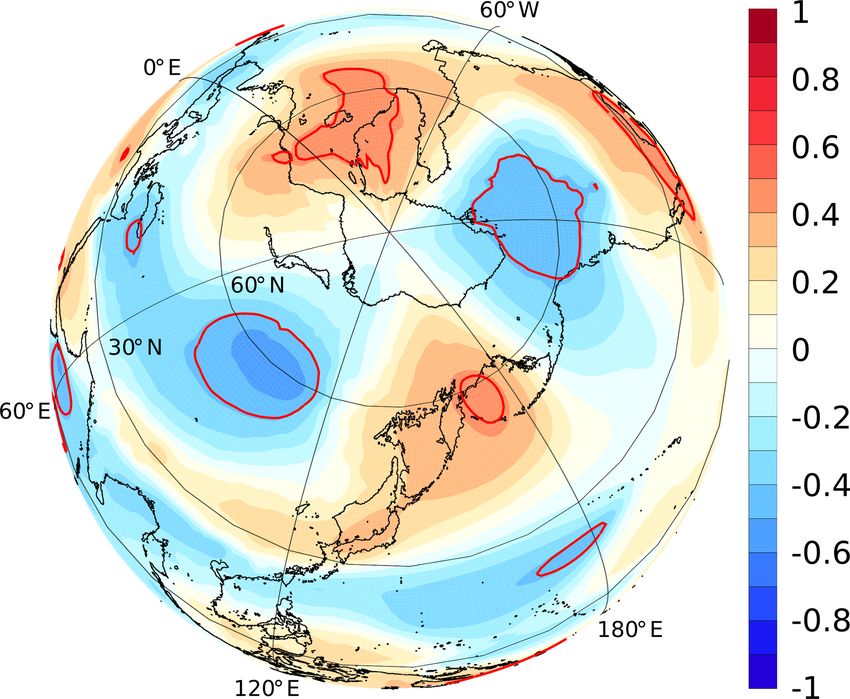
372                                                         P. Bakker et al.: Hypersensitivity of glacial temperatures in Siberia

and the coastal areas of the Kara Sea. Independent evidence         been proposed as an explanation for a westward migration
from permafrost records (Boucsein et al., 2002; Schirrmeis-         of the Eurasian ice sheets during the last glacial period (Li-
ter, 2002; Hubberten et al., 2004; Wetterich et al., 2011), ma-     akka et al., 2016, and references therein). Through the pre-
rine sediment cores (Darby et al., 2006; Polyak et al., 2004,       cipitation shadow effect, the buildup of the Eurasian ice sheet
2007, 2009; Adler et al., 2009; Backman et al., 2009) and           would lead to dry conditions in Siberia and potentially pre-
dating of mollusk shells (Basilyan et al., 2010) also indicates     vent the buildup of an ice sheet in the area.
that the entire region between the Taymyr Peninsula and the            Another way in which ice sheets can impact the climate is
Chukchi Sea remained ice free and was covered by tundra–            through their steering effect on the large-scale atmospheric
steppe during the LGM and that the last grounded ice impacts        circulation. Broccoli and Manabe (1987) showed that the
in different sectors of this region date back to Marine Isotope     buildup of the North American ice sheets leads to substan-
Stage 6 (MIS 6) or potentially MIS 5 within the dating uncer-       tial changes in the midtropospheric flow, including a split
tainties (Stauch and Gualtieri, 2008). Hence, the existing ge-      of the jet stream around the northern and southern edges of
ological evidence indicates that ice sheets covered large parts     the ice sheet and a resulting increase of summer tempera-
of western Siberia (Svendsen et al., 2004; Patton et al., 2015;     tures over Alaska. Similar impacts of glacial ice sheets on
Ehlers et al., 2018) and the east Siberian continental shelf        large-scale atmospheric circulation were found in a number
(Niessen et al., 2013; Jakobsson et al., 2014, 2016) prior to       of other modeling studies (e.g., Cook and Held, 1988; Roe
the last glacial period, but it remains unclear how often north-    and Lindzen, 2001; Justino et al., 2006; Abe-Ouchi et al.,
eastern Siberia experienced large-scale glaciations during the      2007; Langen and Vinther, 2009; Liakka and Nilsson, 2010;
different glacial periods of the Quaternary. Nonetheless, it        Ullman et al., 2014; Liakka et al., 2016). Generally, these
appears that this far northern region was covered by ice dur-       studies indicate a warming over Alaska as a result of the
ing some glacial periods, while it remained ice free during         growth of the North American ice sheets, but it differs from
others.                                                             one study to the next how far westward this warming ex-
   A number of studies have simulated the eastern Siberian          tends into Siberia. In these modeling studies, the warming
LGM climate and ice-sheet growth (e.g., Krinner et al.,             in Alaska and Siberia is linked to increased poleward heat
2006; Charbit et al., 2007; Ganopolski et al., 2010; Abe-           transport induced by changes in the atmospheric stationary
Ouchi et al., 2013; Beghin et al., 2014; Peltier et al., 2015;      waves and to local feedbacks involving the surface albedo
Liakka et al., 2016). They show widely different results, from      and atmospheric water vapor content (Liakka and Lofver-
ice-free conditions to the buildup of a large ice sheet cover-      strom, 2018). A compilation of LGM temperature recon-
ing most of Siberia, and therefore the correspondence with          structions based on various land proxy data provides support
proxy-based reconstructions ranges from good to very poor.          to these inferences, showing that LGM summer temperatures
   Over the years, a number of possible mechanisms have             in northern Siberia were overall not very different from the
been suggested to explain the lack of an ice sheet covering         relatively mild present-day summer temperatures in the re-
eastern Siberia during the LGM and perhaps therewith also           gion (Meyer et al., 2017).
explain the divergent results of coupled climate–ice-sheet             The lack of an LGM ice cover in northeastern Siberia has
simulations for this region during the LGM. The most widely         often been attributed to the increased atmospheric dust load
discussed mechanisms involve changes in atmospheric dust            and/or a precipitation shadow effect of the Eurasian ice sheet
load, orographic precipitation effects and/or changes in at-        to the west. However, based on these mechanisms alone, one
mospheric circulation driven by the buildup of the North            cannot readily explain the absence of a Siberian ice sheet
American and/or Eurasian ice sheets.                                in some glacial periods, but its presence in others, or recon-
   During glacial times, the atmospheric dust load and dust         structions of Siberian LGM summer temperatures close to
deposition were likely substantially larger, particularly at the    present-day values (Meyer et al., 2017), suggests that these
southern margins of the Northern Hemisphere ice sheets and          processes are likely only part of the story. Existing and new
over Siberia (Harrison et al., 2001; Lambert et al., 2015; Ma-      coupled climate model results can shed light on these in-
howald et al., 1999, 2006). Modeling studies have shown that        triguing geological observations. Here, we show that the in-
the buildup of ice over Siberia can be strongly impacted by         termodel spread of simulated LGM summer temperatures is
the effect of dust on the surface albedo as an increase of dust     exceptionally large in Siberia compared to any other region,
deposition on the snowpack leads to a lowering of the snow          suggesting a high susceptibility of Siberian summer temper-
albedo that in turn leads to higher melt rates (Krinner et al.,     atures to minor changes in boundary conditions or model
2006; Willeit and Ganopolski, 2018).                                formulation, and discuss potential underlying mechanisms
   Continental ice sheets have a strong impact on the climate.      and causes. We argue that this high susceptibility of Siberian
It was already recognized by Sanberg and Oerlemans (1983)           summer temperatures to boundary conditions (hypersensitiv-
that under the influence of a preferred wind direction, an ice      ity) is a major factor for the absence or presence of ice sheets
sheet can create a distinct asymmetry with high precipita-          in different Quaternary glacials.
tion rates at the windward side and low precipitation rates on
the leeward side. This precipitation shadow effect has also

Clim. Past, 16, 371–386, 2020                                                                   www.clim-past.net/16/371/2020/
P. Bakker et al.: Hypersensitivity of glacial temperatures in Siberia                                                         373

2     Methodology                                                  CH4 concentration of 375 ppb is slightly higher than the one
                                                                   used here.
In this study, we combine LGM simulations from the sec-               In the first set of sensitivity experiments, we altered the
ond and third phases of the Paleoclimate Modelling Inter-          imposed LGM ice-sheet boundary conditions. Within the
comparison Project (PMIP2 and PMIP3) with LGM sensitiv-            framework of PMIP4, two LGM ice-sheet reconstructions
ity experiments using the Community Earth System Model             are suggested as boundary conditions for the LGM experi-
(CESM).                                                            ments (Kageyama et al., 2017), namely GLAC-1D (Ivanovic
                                                                   et al., 2016) and ICE-6G (Peltier et al., 2015). When com-
2.1    PMIP experiments                                            paring these two ice-sheet reconstructions, we find substan-
                                                                   tial differences, especially an overall increase of the height
We use 17 LGM coupled climate model simulations from               of the North American ice sheets in ICE-6G compared to
PMIP2 and PMIP3/CMIP5 (Table 1; Braconnot et al., 2007;            GLAC-1D and a lowering of the Eurasian ice sheet (Fig. 5a;
Harrison et al., 2015) and their corresponding pre-industrial      both differences are on the order of 10 % of the total ice-
(PI) control simulations as a reference. LGM boundary con-         sheet height; for more details, see Kageyama et al., 2017).
ditions follow the PMIP2 and PMIP3 protocols and include           Changes in surface roughness resulting from the ice-sheet
reduced greenhouse-gas concentrations, changed astronomi-          changes are highly uncertain and have not been taken into
cal parameters, prescribed continental ice sheets and a lower      account. We performed a set of experiments to investigate
global sea level. Nearly half (7 out of 17) of these simulations   the impact of these two different ice-sheet reconstructions on
include dynamic vegetation, while the remaining use pre-           simulated Siberian LGM temperatures (see “continental ice
scribed PI vegetation (Table 1). See https://pmip2.lsce.ipsl.fr    sheets” set of experiments in Table 2).
(last access: 14 February 2020) and https://pmip3.lsce.ipsl.fr        In the second set of sensitivity experiments, we used
(last access: 14 February 2020) for further details and refer-     two different versions of the atmosphere model, CAM4 and
ences. The analysis of PMIP model output is based on clima-        CAM5, to investigate the importance of the atmospheric
tological means, and all output was regridded to a common          model physics (see “atmospheric model physics” set of ex-
0.9◦ × 1.25◦ horizontal resolution. In order to compare the        periments in Table 2). CAM5 differs from its predecessor be-
sea-level pressure results from different models and between       cause it simulates indirect aerosol radiative effects by includ-
PI and LGM, we removed the respective global mean before           ing full aerosol–cloud interactions. Furthermore, it includes
calculating the anomalies. For the analysis of geopotential        improved schemes for moist turbulence, shallow convection
height fields, only 16 instead of 17 PMIP models are used          and cloud micro- and macrophysics. Finally, while CAM4’s
because PMIP2 LGM geopotential height from ECHAM5-                 grid has 26 vertical levels, in CAM5, four levels were added
MPIOM was not available to us.                                     near the surface for a better representation of boundary layer
                                                                   processes. See Neale et al. (2010) for a more detailed de-
2.2    CESM experiments                                            scription of the atmospheric models used in CESM.
                                                                      Furthermore, the CLM4.0 land model includes the pos-
To study the simulated LGM temperatures in the Siberian            sibility to use a representation of the carbon–nitrogen cycle
region in more detail and to isolate individual mechanisms,        and to calculate the resulting changes in leaf area index, stem
we analyzed a number of sensitivity experiments performed          area index and vegetation heights per plant functional type
with the state-of-the-science coupled climate model CESM           (Lawrence et al., 2011). These changes in the biophysical
(version 1.2; Hurrell et al., 2013). The model includes the        properties of the vegetation cover impact, for instance, evap-
Community Atmosphere Model (CAM), Community Land                   otranspiration and surface albedo. Note that the spatial dis-
Model (CLM4.0), the Parallel Ocean Program (POP2) and              tribution of plant functional types is prescribed in CLM4.0,
the Community Ice Code (CICE4). In all our CESM exper-             which is why the model is sometimes described as a semi-
iments, we use a horizontal resolution of 1.9◦ × 2.5◦ in the       dynamic vegetation model. Nonetheless, for simplicity, we
atmosphere (finite volume core) and land, and a nominal 1◦         will refer to simulations that include carbon–nitrogen dy-
resolution of the ocean (60 levels in the vertical) and sea-ice    namics as “interactive vegetation” simulations in the remain-
models with a displaced North Pole.                                der of this paper. To study the interdependency of interactive
   For the CESM LGM simulations, we followed the most              vegetation and atmospheric model physics, we performed a
recent PMIP protocol (PMIP4; Kageyama et al., 2017),               total of four experiments, with either CAM4 or CAM5 and
including greenhouse-gas concentrations (190 ppm CO2 ,             including or excluding interactive vegetation, that are re-
357 ppb CH4 and 200 ppb N2 O), orbital parameters (eccen-          ferred to as the “interactive vegetation” set of experiments
tricity of 0.019, obliquity of 22.949◦ and perihelion – 180◦       (Table 2).
of 114.42◦ ) and changes in the land–sea distribution and al-         All LGM experiments performed with CESM start from a
titude due to lower sea-level (Di Nezio et al., 2016). In this     previous LGM simulation and are run for at least 200 years
study, we used as default the GLAC-1D LGM ice-sheet re-            to obtain a new surface climate equilibrium. Carbon pools in
construction (Ivanovic et al., 2016). Note that the PMIP4          the litter and soils take centuries to equilibrate. However, we

www.clim-past.net/16/371/2020/                                                                   Clim. Past, 16, 371–386, 2020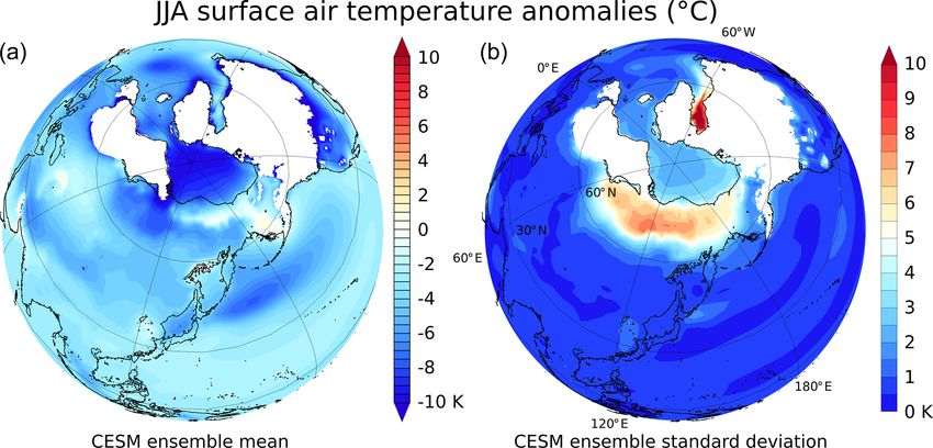
374                                                               P. Bakker et al.: Hypersensitivity of glacial temperatures in Siberia

Table 1. List with PMIP2 and PMIP3 climate models included in the analysis with details on grid resolution and usage of interactive
vegetation. In the last column, the simulated LGM June–July–August (JJA) surface temperature anomaly (K) in the Siberian target region with
respect to the pre-industrial is given for reference. The following abbreviations are used: Atm (atmospheric grid resolution), Ocn (ocean grid
resolution) and L (number of levels in the vertical). See https://pmip2.lsce.ipsl.fr (last access: 14 February 2020) and https://pmip3.lsce.ipsl.fr
(last access: 14 February 2020) for further details and references.

         Model                   Institution                                  Grid resolution             Interactive   PMIP
                                                                                                          vegetation    phase        1T
         CCSM3                   National Center for Atmospheric              Atm: 128 × 64 × L26         No                 2     −3.0
                                 Research, USA                                Ocn: 320 × 384 × L40
         CNRM-CM3.3              Centre National de Recherches                Atm: 256 × 128 × L31        No                 2      12.4
                                 Meteorologiques, France                      Ocn: 362 × 292 × L42
         ECHAM5-MPIOM            Max Planck Institute for Meteorology,        Atm: 96 × 48 × L19          Yes                2     −5.8
                                 Germany                                      Ocn: 120 × 101 × L40
         FGOALS1.0_g             LASG/Institute of                            Atm: 128 × 60 × L26         No                 2    −12.1
                                 Atmospheric Physics, China                   Ocn: 360 × 180 × L33
         HadCM3_AO               UK Met Office Hadley                         Atm: 96 × 72 × L19          No                 2       3.2
                                 Centre, UK                                   Ocn: 288 × 144 × L20
         HadCM3_AOV              UK Met Office Hadley UK                      Atm: 96 × 72 × L19          Yes                2       2.4
                                 Centre, UK                                   Ocn: 288 × 144 × L20
         IPSL-CM4_v1             Institut Pierre Simon                        Atm: 96 × 72 × L19          No                 2     −0.8
                                 Laplace, France                              Ocn: 182 × 149 × L31
         MIROC3.2.2              Center for Climate System Research,          Atm: 128 × 64 × L20         No                 2     −1.9
                                 JAMSTEC, Japan                               Ocn: 256 × 192 × L43
         CCSM4                   National Center for Atmospheric              Atm: 288 × 192 × L26        Yes                3     −7.0
                                 Research, USA                                Ocn: 320 × 384 × L60
         CNRM-CM5                CNRM – C. Européen de Rech.                  Atm: 256 × 128 × L31        No                 3      13.2
                                 Formation Avancée Calcul Sci., France        Ocn: 362 × 292 × L42
         COSMOS-ASO              Max Planck Institute for                     Atm: 96 × 48 × L19          Yes                3     −2.4
                                 Meteorology, Germany                         Ocn: 120 × 101 × L40
         FGOALS_g2               ASG/Institute of Atmospheric                 Atm: 128 × 60 × L26         No                 3    −10.0
                                 Physics, China                               Ocn: 360 × 180 × L30
         GISS-E2-R               NASA Goddard Institute for                   Atm: 144 × 90 × L40         No                 3    −12.4
                                 Space Studies, USA                           Ocn: 288 × 180 × L32
         IPSL-CM5A-LR            Institut Pierre Simon                        Atm: 96 × 96 × L39          Yes                3       3.4
                                 Laplace, France                              Ocn: 182 × 149 × L31
         MIROC-ESM               Center for Climate System Research,          Atm: 128 × 64 × L80         Yes                3       1.9
                                 JAMSTEC, Japan                               Ocn: 256 × 192 × L44
         MPI-ESM-P               Max Planck Institute for                     Atm: 196 × 98 × L47         Yes                3       3.4
                                 Meteorology, Germany                         Ocn: 256 × 220 × L40
         MRI-CGCM3               Meteorological Research                      Atm: 320 × 160 × L48        No                 3       1.1
                                 Institute (MRI), Japan                       Ocn: 364 × 368 × L51

find that the trends are sufficiently small after 200 years to              lations including the carbon–nitrogen cycle are −0.1 and
perform a robust analysis of the surface climate. Changes in                −0.185 Wm−2 using the CAM4 and CAM5 atmospheric
Siberian (global) vegetation carbon pools amount to less than               models, respectively. Climatologies are calculated based on
2 % (0.6 %) of the total PI–LGM change for the model years                  the last 30 years of the simulations. For the sensitivity ex-
150–200. Top-of-the-atmosphere imbalances in the simu-                      periments focusing on interactive vegetation and atmospheric

Clim. Past, 16, 371–386, 2020                                                                              www.clim-past.net/16/371/2020/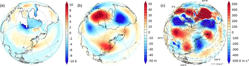
P. Bakker et al.: Hypersensitivity of glacial temperatures in Siberia 375
Table 2. List of simulations included in the three sets of CESM LGM experiments and the PI reference simulations. The following ab-
breviations are used: noVeg indicates no interactive vegetation; Veg indicates including interactive vegetation; PI indicates pre-industrial;
LGM indicates the Last Glacial Maximum; CAM4/5 indicate Community Atmosphere Model version 4 or version 5; GLAC-1D indicates
GLAC-1D ice-sheet reconstruction (Ivanovic et al., 2016); ice6g indicates ICE-6G ice-sheet reconstruction (Peltier et al., 2015).
Experiment Experiment name Atmospheric Interactive Boundary LGM ice-sheet
set model vegetation conditions reconstruction
PI reference PI_CAM4_noVeg CAM4 No PI
simulations PI_CAM5_noVeg CAM5 No PI
PI_CAM4_Veg CAM4 Yes PI
PI_CAM5_Veg CAM5 Yes PI
Continental LGM_CAM5_noVeg CAM5 No LGM GLAC-1D
ice sheets LGM_CAM5_noVeg_ice6g CAM5 No LGM ICE-6G
Atmospheric LGM_CAM4_noVeg CAM4 No LGM GLAC-1D
model physics LGM_CAM5_noVeg CAM5 No LGM GLAC-1D
Interactive LGM_CAM4_noVeg CAM4 No LGM GLAC-1D
vegetation LGM_CAM4_Veg CAM4 Yes LGM GLAC-1D
LGM_CAM5_noVeg CAM5 No LGM GLAC-1D
LGM_CAM5_Veg CAM5 Yes LGM GLAC-1D
model physics, we also performed corresponding PI simula- to as the “Siberian target region” in the remainder of the pa-
tions (Table 2) to enable a proper analysis. Our five CESM per and located roughly between 120–180◦ E and 70–75◦ N),
LGM experiments are jointly referred to as the CESM LGM we see that JJA temperature anomalies averaged over the
ensemble. target region for the individual models range between −12
Throughout this paper, we focus on boreal summer (June– and +12 ◦ C (Fig. 2 and Table 1). The spread in simulated
July–August; JJA) near-surface air temperatures and simply LGM temperatures in the Siberian target region increases
referred to them as “JJA temperatures” in the remainder of compared to PI in all seasons; however, JJA really stands out
this paper. Moreover, when calculating LGM anomalies, we (top row of Fig. A1).
refer to the difference between an LGM simulation and the Disentangling the causes of the particularity of the
corresponding PMIP or CESM PI experiment (Table 2). It Siberian LGM summer temperatures based on PMIP results
is in turn differences between these CESM LGM anomalies is not straightforward because of multiple possible under-
that we use to highlight mechanisms behind the susceptibility lying causes; nonetheless, some aspects can be identified.
of Siberian summer temperatures (Sect. 3.2). Whereas the simulated temperature changes are quite dif-
ferent among PMIP models, a robust decrease in precipita-
tion on the order of 20 %–30 % is simulated (Fig. 1c and d).
3 Results
As a consequence, the (Pearson) correlation between tem-
perature change and precipitation change in the target re-
3.1 Siberian LGM temperatures in PMIP2 and PMIP3
gion is insignificant at the 0.05 significance level (R = 0.36;
ensembles
Fig. 2a; note that, throughout the paper, correlation refers
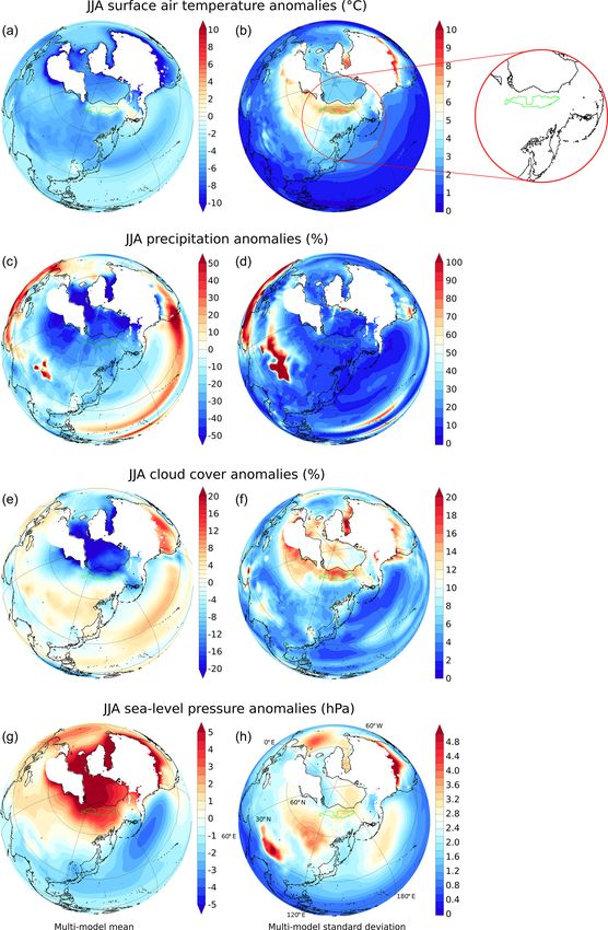
The combined PMIP2 and PMIP3 LGM experiments reveal to intermodel correlation). A significant correlation is found
the particularity of LGM JJA temperatures in Siberia. Of all between temperature and snow cover, with higher temper-
continental areas that were not covered by large ice sheets, atures corresponding to a lower snow cover (R = −0.60;
Siberia shows the largest intermodel spread of LGM anoma- p < 0.05; Fig. 2e). There are similarities between the spa-
lies (standard deviation; Fig. 1b). Another striking feature of tial patterns of the PMIP multi-model spread in tempera-
the Siberian region is that it is one of the few regions where ture anomalies and cloud cover anomalies (Fig. 1b and f);
the PMIP multi-model mean temperature anomaly is close however, within the Siberian target region, local JJA tem-
to or even above zero in some areas, indicating that LGM perature anomalies and cloud cover anomalies are not cor-
summers were potentially as warm as they are at present related at the 0.05 significance level (R = −0.45; Fig. 2b),
(Fig. 1a). Taken together, PMIP simulations show LGM JJA arguing against a leading role of local cloud dynamics to ex-
temperatures in Siberia ranging from warmer to substantially plain the large intermodel spread in Siberian temperatures.
colder than they are at present. If we define a target region As in Yanase and Abe-Ouchi (2007), we find that a weaken-
for Siberia based on the area where the PMIP multi-model ing of the North Pacific high during JJA is a consistent fea-
spread is larger than 7 ◦ C (green contours in Fig. 1; referred ture of PMIP LGM simulations (Fig. 1g). Moreover, a strong
www.clim-past.net/16/371/2020/ Clim. Past, 16, 371–386, 2020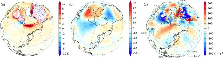
376                                                            P. Bakker et al.: Hypersensitivity of glacial temperatures in Siberia

Figure 1. The PMIP2 and PMIP3 multi-model mean (left panels) and multi-model standard deviation (right panels) in LGM JJA climate
anomalies. (a–b) Temperature anomalies (◦ C). (c–d) Precipitation anomalies (%). (e–f) Cloud cover anomalies (%); (g–h) sea-level pressure
anomalies (hPa). All anomalies are calculated with respect to PI. Note that regions covered by continental ice sheets during the LGM have
been masked out. The green contour (shown in magnification in the top right) shows the Siberian target region, defined here as the region in
which the PMIP multi-model standard deviation is larger than 7 ◦ C. The LGM coastlines are given in black.

Clim. Past, 16, 371–386, 2020                                                                         www.clim-past.net/16/371/2020/

P. Bakker et al.: Hypersensitivity of glacial temperatures in Siberia                                                                         377

Figure 2. PMIP2 and PMIP3 LGM JJA climate anomalies averaged over the northeast Siberian target region. Red (green) numbers refer to
the individual PMIP2 (PMIP3) experiments listed in the lower right. (a) Precipitation anomalies (mm month−1 ) versus temperature anomalies
(◦ C). (b) Cloud cover anomalies (%) versus temperature anomalies (◦ C). (c) Sea-level pressure anomalies (Pa) versus temperature anomalies
(◦ C). (d) Sea-level pressure anomalies (Pa) versus cloud cover anomalies (%). (e) Snow cover anomalies (%) versus temperature anomalies
(K). Black lines show linear fit and the R value (Pearson correlation coefficient) as listed in the lower left corners of the different subfigures.
R values above 0.49 or below −0.49 indicate a significant correlation (p < 0.05; t test).

www.clim-past.net/16/371/2020/                                                                               Clim. Past, 16, 371–386, 2020
378                                                          P. Bakker et al.: Hypersensitivity of glacial temperatures in Siberia

anticorrelation is found in the PMIP LGM simulations be-
tween JJA temperature and sea-level pressure anomalies over
the Siberian target region (R = −0.72; p < 0.05; Fig. 2c): a
more positive temperature anomaly locally creates a thermal
low and hence corresponds to a less pronounced sea-level
pressure anomaly. Concurrently, higher sea-level pressure
anomalies correspond to more positive cloud cover anoma-
lies (R =0.50; p < 0.05; Fig. 2d). Liakka et al. (2016) found
in their model that higher pressure is associated with lower
cloud cover that in turn leads to an increase in JJA tempera-
tures, but our results suggest that this is not the leading mech-
anism in the majority of PMIP LGM results. Inspecting the
PI and LGM seasonal cycles for cloud and snow cover, we
find that also for these variables the changes in intermodel
spread in Siberia are most pronounced in summer. In con-
trast, the intermodel spread in precipitation does not change
                                                                     Figure 3. PMIP2 and PMIP3 linear correlations between JJA
much between PI and LGM (Fig. A1).
                                                                     500 hPa stationary wave geopotential height anomalies at any given
   The strong negative correlation between JJA temperature
                                                                     location and JJA temperature anomalies averaged over the Siberian
and sea-level pressure anomalies suggests that the sea-level         target region (see Fig. 1 for the definition). Anomalies are calcu-
pressure changes could be a consequence of local temper-             lated with respect to PI, and zonal mean geopotential height fields
ature changes. Indeed, another reason for the negative cor-          are subtracted before calculating the anomalies. The red contours
relation could be a remote forcing through anomalous heat            bound the areas for which the correlation is significant (p < 0.1).
advection into the Siberian target region. We find evidence          The LGM coastlines are given in black.
for such a remote forcing of the temperature variations in
the Siberian target region in the significant correlation with
the large-scale mid- to high-latitude stationary wave pat-              Despite the fact that our total CESM LGM ensemble is
tern, resembling a wavenumber 2 structure (Fig. 3). Increased        smaller than the PMIP ensemble (n = 5 instead of n = 17)
Siberian JJA temperatures correspond to a lowering (increas-         and that it was not designed to mimic the PMIP ensem-
ing) of the JJA 500 hPa geopotential height to the southwest         ble, we find that the spread in the CESM LGM temperature
(southeast) of the region. The remote forcing of Siberian tem-       anomalies is surprisingly similar to the PMIP multi-model
peratures can thus be the result of an increase in northward-        spread, both in terms of spatial distribution as well as mag-
flowing relatively warm air masses over the eastern part of          nitude (Fig. 4b). This gives us confidence that investigating
the Asian continent into the region of interest.                     the causes of the sensitivity of northeastern Siberian tem-
   A deeper understanding of the large multi-model spread in         peratures in the CESM ensemble can provide insights into
PMIP LGM JJA temperatures over Siberia and of the mech-              the PMIP intermodel differences. JJA temperatures in the
anisms proposed above is hampered by a multitude of differ-          Siberian target region for the individual CESM experiments
ences between PMIP simulations: different model formula-             are listed in Table 3.
tions, different parts of the climate system that are included          First, we analyze the first set of experiments (“con-
and different boundary conditions including the uncertainty          tinental ice sheets”), differing only in the imposed ice-
in the reconstructed LGM ice sheet and continental outlines.         sheet boundary conditions, namely LGM experiments
Moreover, certain key climate variables are not available for        forced by the GLAC-1D (LGM_CAM5_noVeg) or ICE-6G
a sufficiently large number of the PMIP models. In the fol-          (LGM_CAM5_noVeg_ice6g) ice-sheet reconstructions (Ta-
lowing, we will therefore investigate a purpose-built CESM-          ble 2). On a large scale, using the GLAC-1D ice-sheet recon-
based ensemble of LGM simulations with clearly defined               struction leads to a smaller LGM JJA temperature anomaly
differences between the individual sets of sensitivity experi-       in the Northern Hemisphere (−6.4 ◦ C) than the simulation
ments.                                                               that includes the ICE-6G ice-sheet reconstruction (−7.2 ◦ C;
                                                                     Fig. 5a). Especially in the northeastern Siberian target re-
3.2   Siberian LGM temperatures in the CESM ensemble
                                                                     gion, the LGM simulation using GLAC-1D ice sheets is sub-
                                                                     stantially warmer (9.0 ◦ C) compared to the simulation us-
We construct three sets of LGM sensitivity experiments per-          ing ICE-6G (6.0 ◦ C; Table 3). This can only be caused by
formed with the CESM climate model in order to investi-              changes in the large-scale atmospheric circulation since the
gate in more detail the impact of changes in boundary con-           simulations are identical apart from the ice sheets over North
ditions (continental ice sheets), model formulations (atmo-          America and Eurasia. In line with the PMIP simulations, we
spheric model physics) and including different components            find that higher JJA temperatures in the Siberian target re-
of the climate system (interactive vegetation; Table 2).             gion correspond to specific changes in the 500 hPa geopo-

Clim. Past, 16, 371–386, 2020                                                                     www.clim-past.net/16/371/2020/
P. Bakker et al.: Hypersensitivity of glacial temperatures in Siberia 379
Table 3. Simulated CESM PI and LGM climatic conditions in the Siberian target region. For the abbreviations, see Table 2. Note that LGM
JJA sea-level pressure shown here has been corrected for LGM–PI differences in global mean sea-level pressure.
Experiment name JJA JJA JJA cloud JJA sea-level Minimum JJA snow
temperatures precipitation cover pressure snow cover cover
(◦ C) (mm month−1 ) (%) (hPa) (%) (%)
PI reference PI_CAM4_noVeg 8.0 5.5 55.1 1009 1.3 10.9
simulations PI_CAM5_noVeg 10.7 3.1 65.7 1012 0.0 1.7
PI_CAM4_Veg 6.5 6.7 54.2 1009 2.8 23.1
PI_CAM5_Veg 8.4 6.5 62.4 1013 0.4 13.9
LGM LGM_CAM4_noVeg 8.5 4.2 45.4 1010 0.6 5.8
simulations LGM_CAM5_noVeg 9.0 7.4 62.6 1011 0.6 4.5
LGM_CAM4_Veg 1.4 10.5 46.8 1011 16.8 43.7
LGM_CAM5_Veg −12.1 20.3 70.4 1019 100.0 100.0
LGM_CAM5_noVeg_ice6g 6.0 11.4 58.2 1013 2.5 9.6
Figure 4. CESM ensemble mean (a) and ensemble standard deviation (b) of LGM JJA temperature anomalies (◦ C). Note that regions
covered by continental ice sheets during the LGM have been masked out. The LGM coastlines are given in black.
tential height field, with negative anomalies to the southwest CESM “continental ice sheets” set of experiments (Table 3)
and positive anomalies to the southeast (Fig. 5b), and that as well as in the PMIP results (Fig. 2c).
this stationary wave pattern results in anomalous 500 hPa The second set of CESM LGM simulations (“atmospheric
southerly winds into the target region and a corresponding model physics”) is comprised of simulations in which dif-
anomalous northward heat transport almost all the way from ferent versions of the atmospheric model were used (CAM4
30◦ N to the North Pole (Fig. 5c). We thus find a high sensi- or CAM5; Table 2). Between the LGM_CAM4_noVeg and
tivity of Siberian JJA temperatures with respect to relatively LGM_CAM5_noVeg simulations, we find changes in the
minor changes in the continental ice-sheet geometries, which large-scale atmospheric circulation, in particular the station-
in turn induce changes in the circumpolar stationary wave ary waves, and northward heat transport into Siberia (Fig. 6)
pattern and anomalous northward heat transport in CESM. that are broadly similar to the response to different ice sheets
The similarity of the associated temperature and geopoten- as described above. Similar to the analysis of the PMIP mod-
tial height anomaly patterns (wavenumber 2 structure; Fig. 5) els (Fig. 3) and the CESM “continental ice sheets” set of ex-
with the PMIP-based response (Figs. 1 and 3) suggests that periments (Fig. 5), we find that using different atmospheric
this mechanism could also explain part of the spread in PMIP model physics can lead to JJA warming (cooling) in the
simulations. The anomalous northward heat transport we see Siberian target region in response to enhanced (decreased)
in the stationary waves contributes to reinforce the (clima- meridional heat transport into northeastern Siberia. Interest-
tological) thermal low over Siberia and explains the nega- ingly, if we look in more detail, we find that the resulting sur-
tive relationship between JJA temperature and JJA surface face temperature changes in Siberia are more complex in the
pressure anomalies in the Siberian target region, both in the “atmospheric model physics” set of experiments than they
are for the experiments described previously. There is warm-
www.clim-past.net/16/371/2020/ Clim. Past, 16, 371–386, 2020380 P. Bakker et al.: Hypersensitivity of glacial temperatures in Siberia Figure 5. Impact of the prescribed LGM ice-sheet topography (GLAC-1D versus ICE-6G) on simulated LGM climate anomalies during the boreal summer season (JJA). Results are shown as the CESM experiment LGM_CAM5_noVeg minus LGM_CAM5_noVeg_ice6g. (a) Near- surface temperature anomalies (K). (b) The 500hPa geopotential height anomalies (m; anomalies calculated after subtracting the zonal mean). (c) Vertically averaged meridional sensible heat transport anomalies (K ms−1 ; shading). Vectors in panel (c) show 500 hPa wind anomalies (ms−1 ). In panel (a), regions covered by continental ice sheets during the LGM have been masked out. The red (blue) contours in panel (a) depict positive (negative) differences in ice-sheet height (m) between the GLAC-1D and ICE-6G reconstructions (GLAC-1D – ICE-6G; 300 m contour interval). The LGM coastlines are given in black. Figure 6. Impact of using different atmospheric models (CAM5 versus CAM4) on simulated LGM climate anomalies during the boreal summer season (JJA). Results are shown as LGM–PI anomalies for LGM_ CAM5_noVeg minus LGM_CAM4_noVeg. (a) Near-surface temperature anomalies (K). (b) 500 hPa stationary wave geopotential height anomalies (m; anomalies calculated after subtracting the zonal mean). (c) Vertically averaged meridional sensible heat transport anomalies (K m s−1 ; shading). Vectors in panel (c) show 500 hPa wind anomalies (ms−1 ). In panel (a), regions covered by continental ice sheets during the LGM have been masked out. The LGM coastlines are given in black. ing in some parts of the region but also cooling in other parts dynamics; thus, the described mechanism in this CESM “at- (Fig. 6a), and there are differences in the stationary wave mospheric model physics” set of experiments could as well pattern and in meridional heat transport. This is possibly re- explain (part of) the spread within the PMIP ensemble. lated to slight shifts in the centers of action in the geopoten- An important element in the high-latitude climate system tial height anomalies and resulting changes in the air masses is the vegetation–climate feedback. In the PMIP ensemble, that enter the Siberian target region. This highlights the com- 7 out of 17 models include the vegetation–climate feedback plexity of comparing simulations with different atmospheric (Table 1). However, a systematic difference in simulated JJA model versions that not only differ in their response of the LGM temperature anomalies for the Siberian region could large-scale atmospheric circulation to LGM boundary condi- not be found when comparing models with vegetation feed- tions but also exhibit different local feedbacks with changes back with those that did not include this additional feedback. in cloud cover, humidity and pressure, which are directly in- This does not come as a surprise if one considers the rela- fluenced by, for instance, differences in cloud parameteriza- tively small sample size with respect to all the intermodel tions and radiative properties of the atmosphere. This point differences that impact the simulated LGM JJA tempera- is further exemplified by the substantial differences between tures. We performed PI and LGM simulations with CESM CAM4 and CAM5 in Siberian JJA temperatures and snow including and excluding interactive vegetation (the “interac- cover under PI conditions (Table 3). The models in the PMIP tive vegetation” set; Table 2) to investigate its importance for ensemble all differ in the included atmospheric physics and Siberian temperatures. We find that the vegetation–climate Clim. Past, 16, 371–386, 2020 www.clim-past.net/16/371/2020/
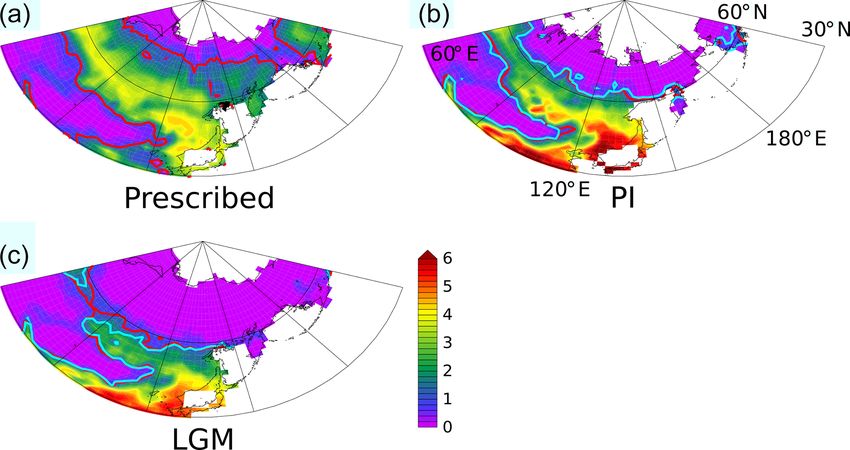
P. Bakker et al.: Hypersensitivity of glacial temperatures in Siberia                                                                    381

Figure 7. JJA LGM temperature anomalies showing the impact of introducing vegetation–climate feedbacks. Results are shown as LGM–PI
anomalies for CAM4 (a) LGM_CAM4_Veg – LGM_CAM4_noVeg and CAM5 (b) LGM_CAM5_Veg – LGM_CAM5_noVeg. Regions
covered by continental ice sheets during the LGM have been masked out. The LGM coastlines are given in black. Note the different scaling
used for the two panels.

Figure 8. Leaf area index (m2 m−2 ) in northeastern Asia as prescribed in the simulations without interactive vegetation (a), and as simulated
in the pre-industrial (b) and LGM (c) CAM4_Veg experiments including interactive vegetation. Contours give the leaf area index of 1 m2 m−2
(red for CAM4 and light blue for CAM5).

feedback leads to a large LGM JJA cooling over Siberia,                  of the tree and shrub limits. This relationship between veg-
which is even more pronounced when using the CAM5 at-                    etation and snow cover also determines the resulting LGM
mospheric model instead of CAM4 (Fig. 7 and Table 3).                    JJA temperature changes (compare Fig. 7a and c; Table 3).
If vegetation is allowed to respond to the changing climate              Previous studies also found an important role of vegetation
through carbon–nitrogen dynamics, the tree and shrub limits              feedbacks in defining LGM Arctic temperatures (Jahn et al.,
shift south by several degrees of latitude as shown by the leaf          2005). The impact of interactive vegetation in CESM is also
area index (Fig. 8a and c). In CESM, the presence of vegeta-             clearly seen in the PI simulations, resulting in a substantial
tion, its height as well as its density have a large impact on           decrease in the leaf area index with respect to the prescribed
the surface albedo through the vegetation–albedo feedback:               values (Fig. 8a and b) and is in line with the cold bias in mod-
vegetation that protrudes through the snowpack lowers the                eled Siberian surface temperatures described by Lawrence
surface albedo that in turn leads to a positive feedback loop            et al. (2011) (see also Table 3).
with increasing temperatures, more snowmelt, more vegeta-                   Looking at all the experiments in the third set of ex-
tion growth and an even lower surface albedo. Accordingly,               periments (“interactive vegetation”; Table 2), using differ-
the situation in the CESM simulations including interactive              ent atmospheric model physics (Fig. 6) with or without in-
vegetation is such that the cold and snow-covered landscape              teractive vegetation (Fig. 7), we find that the strong cool-
limits vegetation growth and leads to a southward migration              ing in Siberia in the simulation that combines both the dif-

www.clim-past.net/16/371/2020/                                                                            Clim. Past, 16, 371–386, 2020
382                                                        P. Bakker et al.: Hypersensitivity of glacial temperatures in Siberia

ferent atmospheric model physics and interactive vegetation        atmospheric stationary wave patterns drive Siberian JJA tem-
(LGM_CAM5_Veg; Fig. 7b) is not readily explained as a lin-         peratures directly through local cloud changes.
ear combination of the two individual effects. This is true for       Although situated at high northern latitudes, geological
Siberian JJA temperatures but also for other key climate vari-     evidence suggests that Siberia was covered by continental
ables (Table 3). It should be noted that the simulations with      ice sheets during some glacial periods but remained largely
the lowest JJA LGM temperatures in Table 3 are in fact the         ice free during others, for instance, the last glacial period
ones with the highest precipitation rates (not only in JJA but     including the LGM. Increased atmospheric dust deposition
also in the annual mean; not shown). This all shows the com-       and a precipitation shadow cast by the Eurasian ice sheets
plexity of the response to a combination of factors, in this       to the west are often listed as possible causes; however,
case changes in large-scale atmospheric circulation, local at-     such mechanisms cannot readily explain the absence of a
mospheric processes and local land-surface processes. It is to     Siberian ice sheet in some glacial periods but its presence
be expected that the response of individual PMIP simulations       in others, or conform with the independent reconstructions
is similarly complex.                                              of Siberian LGM summer temperatures close to present-day
                                                                   values (Meyer et al., 2017). This is suggesting that these pro-
                                                                   cesses are likely only part of the story, and here we argue for
4   Concluding remarks                                             the importance of changes in meridional atmospheric heat
                                                                   transport and the configuration of the Northern Hemisphere
From a climate model perspective, LGM JJA temperatures             continental ice sheets in order to understand the geological
in northeastern Siberia appear highly susceptible to changes       evidence. The combination of these factors, accompanied by
in the imposed boundary conditions, included feedbacks and         local feedbacks can lead to strongly divergent summer tem-
processes, and the model physics of the different climate          peratures in the region, which during some glacial periods
model components, much more so for Siberia than for any            could have been sufficiently low to allow for the buildup of
other region. This becomes apparent from the comparison of         an ice sheet, while during other glacials, above-freezing sum-
17 different PMIP2 and PMIP3 LGM experiments, as well              mer temperatures might have prevented a multi-year snow-
as from three sets of CESM sensitivity experiments. The            pack, and hence an ice sheet, from forming. Finally, this high
spread in Siberian JJA LGM temperature anomalies in the            sensitivity of Siberian LGM summer temperatures in differ-
CESM ensemble is ∼ 20 ◦ C, which is comparable to the in-          ent climate models will present a major challenge in future
termodel spread of ∼ 24 ◦ C found in the PMIP simulations.         modeling efforts using coupled ice-sheet–climate models.
The main cause appears to be that relatively small changes
in the continental ice sheets or model physics can lead to
large changes in meridional atmospheric heat transport re-
lated to changes in the circumpolar atmospheric stationary
wave pattern, in line with Ullman et al. (2014) and Liakka
and Lofverstrom (2018). Local snow–albedo and vegetation–
climate feedbacks strongly amplify the Siberian JJA temper-
ature change. Recently, Schenk et al. (2018) showed that the
spatial resolution of the atmospheric model is key to obtain-
ing realistic glacial temperature anomalies. However, we do
not find any correlation between atmospheric model resolu-
tion and Siberian JJA LGM temperature anomalies (Table 1),
despite having some models with a resolution very similar
to the one used by Schenk et al. (2018). We note, however,
that we did not perform a dedicated sensitivity experiment,
changing only the spatial resolution while keeping all other
factors the same.
   In most of the examined PMIP LGM simulations, Siberia
receives less precipitation; however, we do not find indica-
tions that the buildup of a Siberian ice sheet was hampered
by the absence of precipitation. On the contrary, in both the
PMIP ensemble and our CESM experiments, we find that lo-
cal precipitation and JJA temperature changes are not signif-
icantly correlated, while cooler summers are strongly corre-
lated to a higher snow cover, suggesting that a cold climate
would be associated with a perennial snow cover. We also
do not find support for the notion that changes in large-scale

Clim. Past, 16, 371–386, 2020                                                                 www.clim-past.net/16/371/2020/
P. Bakker et al.: Hypersensitivity of glacial temperatures in Siberia 383 Appendix A Figure A1. PMIP2 and PMIP3 multi-model mean (left panels) and multi-model standard deviation (right panels) seasonal cycles of selected variables for PI (red), LGM (blue), and LGM anomalies (LGM–PI; black). Mean and standard deviation are calculated for the Siberian target region. Top row: temperatures (◦ C); second row: precipitation (mm yr−1 ); third row: cloud cover (%); bottom row: snow cover (%). www.clim-past.net/16/371/2020/ Clim. Past, 16, 371–386, 2020
384                                                                P. Bakker et al.: Hypersensitivity of glacial temperatures in Siberia

Data availability. For the PMIP experiment results, see https:               on 230Th/U-dating of Mollusk Shells, Structure and Develop-
//pmip2.lsce.ipsl.fr (LSCE, 2020a) and https://pmip3.lsce.ipsl.fr            ment of the Lithosphere, Paulsen, 506–514, 2010.
(LSCE, 2020b) for further details and references. Results from the         Beghin, P., Charbit, S., Dumas, C., Kageyama, M., Roche,
CESM sensitivity experiments can be obtained from the authors.               D. M., and Ritz, C.: Interdependence of the growth of the
                                                                             Northern Hemisphere ice sheets during the last glaciation:
                                                                             the role of atmospheric circulation, Clim. Past, 10, 345–358,
Author contributions. PB and IR designed the study. PB per-                  https://doi.org/10.5194/cp-10-345-2014, 2014.
formed the CESM sensitivity experiments and analyzed the PMIP              Boucsein, B., Knies, J., and Stein, R.: Organic matter deposition
and CESM experiments. PB wrote the manuscript. IR reviewed the               along the Kara and Laptev Seas continental margin ( eastern Arc-
literature for geological and climatological reconstructions. All au-        tic Ocean ) during last deglaciation and Holocene : evidence from
thors participated in the discussion of the results and the manuscript,      organic-geochemical and petrographical data, Mar. Geol., 183,
and provided feedback and comments.                                          67–87, 2002.
                                                                           Braconnot, P., Otto-Bliesner, B., Harrison, S., Joussaume, S., Pe-
                                                                             terchmitt, J.-Y., Abe-Ouchi, A., Crucifix, M., Driesschaert, E.,
Competing interests. The authors declare that they have no con-              Fichefet, Th., Hewitt, C. D., Kageyama, M., Kitoh, A., Laîné,
flict of interest.                                                           A., Loutre, M.-F., Marti, O., Merkel, U., Ramstein, G., Valdes,
                                                                             P., Weber, S. L., Yu, Y., and Zhao, Y.: Results of PMIP2 coupled
                                                                             simulations of the Mid-Holocene and Last Glacial Maximum –
                                                                             Part 1: experiments and large-scale features, Clim. Past, 3, 261–
Acknowledgements. The climate model simulations were car-
                                                                             277, https://doi.org/10.5194/cp-3-261-2007, 2007.
ried out on the supercomputer of the Norddeutscher Verbund
                                                                           Broccoli, A. J. and Manabe, S.: The Effects of the Laurentide
für Hoch- und Höchstleistungsrechnen (HLRN). We thank Pe-
                                                                             Ice Sheet on North American Climate during the Last Glacial
dro diNezio for providing us with CESM LGM initial and boundary
                                                                             Maximum, Géographie physique et Quaternaire, 41, 291–299,
conditions.
                                                                             https://doi.org/10.7202/032684ar, 1987.
                                                                           Charbit, S., Ritz, C., Philippon, G., Peyaud, V., and Kageyama,
                                                                             M.: Numerical reconstructions of the Northern Hemisphere ice
Financial support. This research has been supported by the Ger-              sheets through the last glacial-interglacial cycle, Clim. Past, 3,
man Federal Ministry of Education and Science (BMBF) (PalMod).               15–37, https://doi.org/10.5194/cp-3-15-2007, 2007.
                                                                           Cook, K. H. and Held, I. M.: Stationary Waves of the Ice Age
The article processing charges for this open-access publica-                 Climate, J. Climate, 1, 807–819, https://doi.org/10.1175/1520-
tion were covered by the University of Bremen.                               0442(1988)0012.0.co;2, 1988.
                                                                           Darby, D. A., Polyak, L., and Bauch, H. A.: Progress in Oceanog-
                                                                             raphy Past glacial and interglacial conditions in the Arctic Ocean
Review statement. This paper was edited by Laurie Menviel and                and marginal seas – a review, Prog. Oceanogr., 71, 129–144,
reviewed by two anonymous referees.                                          https://doi.org/10.1016/j.pocean.2006.09.009, 2006.
                                                                           Di Nezio, P. N., Timmermann, A., Tierney, J. E., Jin, F. F., Otto-
                                                                             Bliesner, B. L., Rosenbloom, N., Mapes, B., Neale, R. B.,
References                                                                   Ivanovic, R. F., and Montenegro, A.: The climate response of the
                                                                             Indo-Pacific warm pool to glacial sea level, Paleoceanography,
Abe-Ouchi, A., Segawa, T., and Saito, F.: Climatic Conditions for            31, 866–894, https://doi.org/10.1002/2015PA002890, 2016.
  modelling the Northern Hemisphere ice sheets throughout the ice          Ehlers, J., Gibbard, P. L., and Hughes, P. D.: Quaternary Glacia-
  age cycle, Clim. Past, 3, 423–438, https://doi.org/10.5194/cp-3-           tions and Chronology, in: Past Glacial Environments, edited by:
  423-2007, 2007.                                                            Menzies, J. and van der Meer, J. J. M., chap. 4, Elsevier, 2018.
Abe-Ouchi, A., Saito, F., Kawamura, K., Raymo, M. E., Okuno,               Ganopolski, A., Calov, R., and Claussen, M.: Simulation of
  J., Takahashi, K., and Blatter, H.: Insolation-driven 100,000-year         the last glacial cycle with a coupled climate ice-sheet
  glacial cycles and hysteresis of ice-sheet volume, Nature, 500,            model of intermediate complexity, Clim. Past, 6, 229–244,
  190–193, https://doi.org/10.1038/nature12374, 2013.                        https://doi.org/10.5194/cp-6-229-2010, 2010.
Adler, R. E., Polyak, L., Ortiz, J. D., Kaufman, D. S., Channell,          Gualtieri, L., Vartanyan, S. L., Brigham-Grette, J., and Ander-
  J. E. T., Xuan, C., Grottoli, A. G., Sellén, E., and Crawford,             son, P. M.: Evidence for an ice-free Wrangel Island, northeast
  K. A.: Sediment record from the western Arctic Ocean with                  Siberia during the Last Glacial Maximum, Boreas, 34, 264–273,
  an improved Late Quaternary age resolution : HOTRAX core                   https://doi.org/10.1080/03009480510013097, 2005.
  HLY0503-8JPC, Mendeleev Ridge, Global Planet. Change, 68,                Harrison, S. P., Kohfeld, K. E., Roelandt, C., and Claquin,
  18–29, https://doi.org/10.1016/j.gloplacha.2009.03.026, 2009.              T.: The role of dust in climate changes today, at the last
Backman, J., Fornaciari, E., and Rio, D.: Marine Micropale-                  glacial maximum and in the future, Earth-Sci. Rev., 54, 43–80,
  ontology Biochronology and paleoceanography of late Pleis-                 https://doi.org/10.1016/S0012-8252(01)00041-1, 2001.
  tocene and Holocene calcareous nannofossil abundances                    Harrison, S. P., Bartlein, P. J., Izumi, K., Li, G., Annan,
  across the Arctic Basin, Mar. Micropaleontol., 72, 86–98,                  J. D., Hargreaves, J. C., Braconnot, P., and Kageyama,
  https://doi.org/10.1016/j.marmicro.2009.04.001, 2009.                      M.: Evaluation of CMIP5 palaeo-simulations to im-
Basilyan, A. E., Nikolsky, P. A., Maksimov, F. E., and Kuznetsov,
  V. Y.: Age of Cover Glaciation of the New Siberian Islands Based

Clim. Past, 16, 371–386, 2020                                                                            www.clim-past.net/16/371/2020/
P. Bakker et al.: Hypersensitivity of glacial temperatures in Siberia 385 prove climate projections, Nat. Clim. Change, 5, 735–743, and PMIP4 sensitivity experiments, Geosci. Model Dev., 10, https://doi.org/10.1038/nclimate2649, 2015. 4035–4055, https://doi.org/10.5194/gmd-10-4035-2017, 2017. Hubberten, H. W., Andreev, A., Astakhov, V. I., Demi- Kleman, J., Fastook, J., Ebert, K., Nilsson, J., and Caballero, dov, I., Dowdeswell, J. A., Henriksen, M., Hjort, C., R.: Pre-LGM Northern Hemisphere ice sheet topography, Houmark-nielsen, M., Jakobsson, M., Kuzmina, S., Larsen, Clim. Past, 9, 2365–2378, https://doi.org/10.5194/cp-9-2365- E., Pekka, J., Lys, A., Saarnisto, M., Schirrmeister, L., 2013, 2013. Sher, A. V., Siegert, C., Siegert, M. J., and Inge, J.: The Krinner, G., Boucher, O., and Balkanski, Y.: Ice-free glacial north- periglacial climate and environment in northern Eurasia dur- ern Asia due to dust deposition on snow, Clim. Dynam., 27, 613– ing the Last Glaciation, Quaternary Sci. Rev., 23, 1333–1357, 625, https://doi.org/10.1007/s00382-006-0159-z, 2006. https://doi.org/10.1016/j.quascirev.2003.12.012, 2004. Laboratoire des sciences du climat et de l’environnement (LSCE): Hurrell, J. W., Holland, M. M., Gent, P. R., Ghan, S., Kay, J. E., Paleoclimate Modelling Intercomparison Project Phase II, avail- Kushner, P. J., Lamarque, J. F., Large, W. G., Lawrence, D. M., able at: https://pmip2.lsce.ipsl.fr, last access: 14 February 2020a. Lindsay, K., Lipscomb, W. H., Long, M. C., Mahowald, N. M., Laboratoire des sciences du climat et de l’environnement (LSCE): Marsh, D. R., Neale, R. B., Rasch, P., Vavrus, S., Vertenstein, Paleoclimate Modelling Intercomparison Project Phase III, avail- M., Bader, D. A., Collins, W. D., Hack, J. J., Kiehl, J., and Mar- able at: https://pmip3.lsce.ipsl.fr, last access: 14 February 2020b. shall, S.: The community earth system model: A framework for Lambert, F., Tagliabue, A., Shaffer, G., Lamy, F., Winckler, collaborative research, B. Am. Meteorol. Soc., 94, 1339–1360, G., Farias, L., Gallardo, L., and Pol-Holz, R. D.: Dust https://doi.org/10.1175/BAMS-D-12-00121.1, 2013. fluxes and iron fertilization in Holocene and Last Glacial Ivanovic, R. F., Gregoire, L. J., Kageyama, M., Roche, D. M., Maximum climates, Geophys. Res. Lett., 42, 6014–6023, Valdes, P. J., Burke, A., Drummond, R., Peltier, W. R., and https://doi.org/10.1002/2015GL064250, 2015. Tarasov, L.: Transient climate simulations of the deglaciation 21– Langen, P. L. and Vinther, B. M.: Response in atmospheric 9 thousand years before present (version 1) – PMIP4 Core exper- circulation and sources of Greenland precipitation to iment design and boundary conditions, Geosci. Model Dev., 9, glacial boundary conditions, Clim. Dynam., 32, 1035–1054, 2563–2587, https://doi.org/10.5194/gmd-9-2563-2016, 2016. https://doi.org/10.1007/s00382-008-0438-y, 2009. Jahn, A., Claussen, M., Ganopolski, A., and Brovkin, V.: Lawrence, D. M., Oleson, K. W., Flanner, M. G., Thornton, P. E., Quantifying the effect of vegetation dynamics on the cli- Swenson, S. C., Lawrence, P. J., Zeng, X., Yang, Z.-L., Levis, S., mate of the Last Glacial Maximum, Clim. Past, 1, 1–7, Sakaguchi, K., Bonan, G. B., and Slater, A. G.: Parameterization https://doi.org/10.5194/cp-1-1-2005, 2005. improvements and functional and structural advances in Version Jakobsson, M., Andreassen, K., Rún, L., Dove, D., Dowdeswell, 4 of the Community Land Model, J. Adv. Model. Earth Sy., 3, J. A., England, J. H., Funder, S., Hogan, K., Ingólfsson, Ó., 1–27, https://doi.org/10.1029/2011ms000045, 2011. Jennings, A., Krog, N., Kirchner, N., Landvik, J. Y., Mayer, Liakka, J. and Lofverstrom, M.: Arctic warming induced by the L., Mikkelsen, N., Möller, P., Niessen, F., Nilsson, J., Re- Laurentide Ice Sheet topography, Clim. Past, 14, 887–900, gan, M. O., Polyak, L., and Nørgaard-pedersen, N.: Arc- https://doi.org/10.5194/cp-14-887-2018, 2018. tic Ocean glacial history, Quaternary Sci. Rev., 92, 40–67, Liakka, J. and Nilsson, J.: The impact of topographically forced https://doi.org/10.1016/j.quascirev.2013.07.033, 2014. stationary waves on local ice-sheet climate, J. Glaciol., 56, 534– Jakobsson, M., Nilsson, J., Anderson, L. G., Backman, J., Björk, 544, https://doi.org/10.3189/002214310792447824, 2010. G., Cronin, T. M., Kirchner, N., Koshurnikov, A., Mayer, L., Liakka, J., Löfverström, M., and Colleoni, F.: The impact of the Noormets, R., O’Regan, M., Stranne, C., Ananiev, R., Bar- North American glacial topography on the evolution of the rientos Macho, N., Cherniykh, D., Coxall, H., Eriksson, B., Eurasian ice sheet over the last glacial cycle, Clim. Past, 12, Flodén, T., Gemery, L., Gustafsson, Ö., Jerram, K., Johans- 1225–1241, https://doi.org/10.5194/cp-12-1225-2016, 2016. son, C., Khortov, A., Mohammad, R., and Semiletov, I.: Ev- Mahowald, N., Kohfeld, K., Hansson, M., Balkanski, Y., Harrison, idence for an ice shelf covering the central Arctic Ocean S. P., Prentice, I. C., Schulz, M., and Rodhe, H.: Dust sources and during the penultimate glaciation, Nat. Commun., 7, 1–10, deposition during the last glacial maximum and current climate: https://doi.org/10.1038/ncomms10365, 2016. A comparison of model results with paleodata from ice cores and Justino, F., Timmermann, A., Merkel, U., and Peltier, W. R.: An marine sediments, J. Geophys. Res.-Atmos., 104, 15895–15916, initial intercomparison of atmospheric and oceanic climatology https://doi.org/10.1029/1999jd900084, 1999. for the ICE-5G and ICE-4G models of LGM paleotopography, J. Mahowald, N. M., Yoshioka, M., Collins, W. D., Conley, Climate, 19, 3–14, https://doi.org/10.1175/JCLI3603.1, 2006. A. J., Fillmore, D. W., and Coleman, D. B.: Climate re- Kageyama, M., Albani, S., Braconnot, P., Harrison, S. P., Hopcroft, sponse and radiative forcing from mineral aerosols dur- P. O., Ivanovic, R. F., Lambert, F., Marti, O., Peltier, W. R., Pe- ing the last glacial maximum, pre-industrial, current and terschmitt, J.-Y., Roche, D. M., Tarasov, L., Zhang, X., Brady, E. doubled-carbon dioxide climates, Geophys. Res. Lett., 33, 2–5, C., Haywood, A. M., LeGrande, A. N., Lunt, D. J., Mahowald, N. https://doi.org/10.1029/2006GL026126, 2006. M., Mikolajewicz, U., Nisancioglu, K. H., Otto-Bliesner, B. L., Meyer, V. D., Hefter, J., Lohmann, G., Max, L., Tiedemann, R., and Renssen, H., Tomas, R. A., Zhang, Q., Abe-Ouchi, A., Bartlein, Mollenhauer, G.: Summer temperature evolution on the Kam- P. J., Cao, J., Li, Q., Lohmann, G., Ohgaito, R., Shi, X., Volodin, chatka Peninsula, Russian Far East, during the past 20 000 E., Yoshida, K., Zhang, X., and Zheng, W.: The PMIP4 contri- years, Clim. Past, 13, 359–377, https://doi.org/10.5194/cp-13- bution to CMIP6 – Part 4: Scientific objectives and experimental 359-2017, 2017. design of the PMIP4-CMIP6 Last Glacial Maximum experiments www.clim-past.net/16/371/2020/ Clim. Past, 16, 371–386, 2020
You can also read


