Spatial Capture-Recapture for Categorically Marked Populations with An Application to Genetic Capture-Recapture - bioRxiv
←
→
Page content transcription
If your browser does not render page correctly, please read the page content below

bioRxiv preprint first posted online Feb. 15, 2018; doi: http://dx.doi.org/10.1101/265678. The copyright holder for this preprint
 (which was not peer-reviewed) is the author/funder, who has granted bioRxiv a license to display the preprint in perpetuity.
                              It is made available under a CC-BY-NC-ND 4.0 International license.

        Spatial Capture-Recapture for Categorically Marked
           Populations with An Application to Genetic
                        Capture-Recapture
                                       Ben C. Augustinea
                                       J. Andrew Royleb
                                       Sean M. Murphyc
                                     Richard B. Chandlerd
                                          John J. Coxe
                                       Marcella J. Kellya
     a
       Department of Fish and Wildlife Conservation, Virginia Tech, Blacksburg, VA 24061
        b
          U.S. Geological Survey, Patuxent Wildlife Research Center, Laurel, MD, 20708
               c
                 New Mexico Department of Game and Fish, Santa Fe, NM, 87504
            d
              Department of Forestry and Natural Resources, University of Georgia,
                                      Athens, GA, 30602
            e
              Department of Forestry, University of Kentucky, Lexington, KY, 40546
                            Corresponding email: baugusti@vt.edu
                                                        February 12, 2018

                                                                       1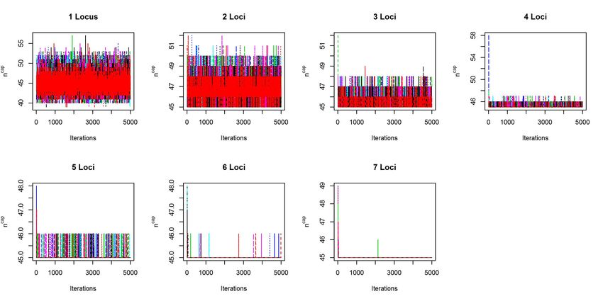
bioRxiv preprint first posted online Feb. 15, 2018; doi: http://dx.doi.org/10.1101/265678. The copyright holder for this preprint
 (which was not peer-reviewed) is the author/funder, who has granted bioRxiv a license to display the preprint in perpetuity.
                              It is made available under a CC-BY-NC-ND 4.0 International license.

                                                                Abstract

   Recently introduced unmarked spatial capture-recapture (SCR), spatial mark-resight (SMR),
   and 2-flank spatial partial identity models (SPIM) extend the domain of SCR to populations
   or observation systems that do not always allow for individual identity to be determined with
   certainty. For example, some species do not have natural marks that can reliably produce
   individual identities from photographs, and some methods of observation produce partial
   identity samples as is the case with remote cameras that sometimes produce single flank
   photographs. These models share the feature that they probabilistically resolve the uncer-
   tainty in individual identity using the spatial location where samples were collected. Spatial
   location is informative of individual identity in spatially structured populations with home
   range sizes smaller than the extent of the trapping array because a latent identity sample
   is more likely to have been produced by an individual living near the trap where it was
   recorded than an individual living further away from the trap. Further, the level of infor-
   mation about individual identity that a spatial location contains is determined by two key
   ecological concepts, population density and home range size. The number of individuals
   that could have produced a latent or partial identity sample increases as density and home
   range size increase because more individual home ranges will overlap any given trap. We
   show this uncertainty can be quantified using a metric describing the expected magnitude
   of uncertainty in individual identity for any given population density and home range size,
   the Identity Diversity Index (IDI). We then show that the performance of latent and partial
   identity SCR models varies as a function of this index and produces imprecise and biased
   estimates in many high IDI scenarios when data are sparse. We then extend the unmarked
   SCR model to incorporate partially identifying covariates which reduce the level of uncer-
   tainty in individual identity, increasing the reliability and precision of density estimates,
   and allowing reliable density estimation in scenarios with higher IDI values and with more
   sparse data. We illustrate the performance of this “categorical SPIM” via simulations and
   by applying it to a black bear data set using microsatellite loci as categorical covariates,

                                                                       2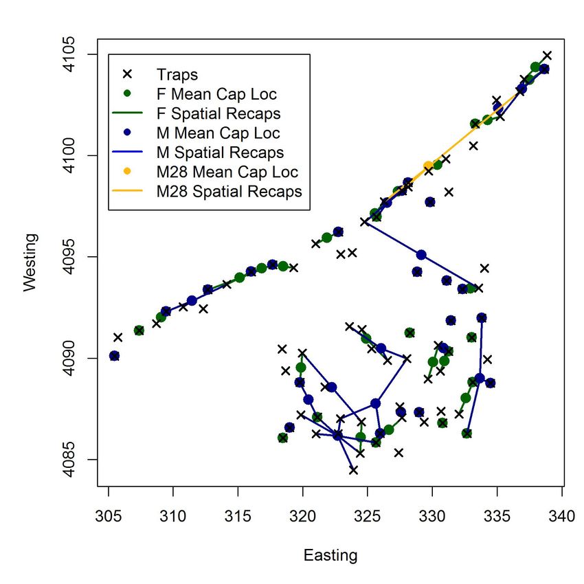
bioRxiv preprint first posted online Feb. 15, 2018; doi: http://dx.doi.org/10.1101/265678. The copyright holder for this preprint
 (which was not peer-reviewed) is the author/funder, who has granted bioRxiv a license to display the preprint in perpetuity.
                              It is made available under a CC-BY-NC-ND 4.0 International license.

   where we reproduce the full data set estimates with only slightly less precision using fewer
   loci than necessary for confident individual identification. The categorical SPIM offers an
   alternative to using probability of identity criteria for classifying genotypes as unique, shift-
   ing the “shadow effect”, where more than one individual in the population has the same
   genotype, from a source of bias to a source of uncertainty. We discuss the difficulties that
   real world data sets pose for latent identity SCR methods, most importantly, individual
   heterogeneity in detection function parameters, and argue that the addition of partial iden-
   tity information reduces these concerns. We then discuss how the categorical SPIM can be
   applied to other wildlife sampling scenarios such as remote camera surveys, where natural
   or researcher-applied partial marks can be observed in photographs. Finally, we discuss how
   the categorical SPIM can be added to SMR, 2-flank SPIM, or other future latent identity
   SCR models.
   Keywords: Spatial capture-recapture, partial identity, unmarked spatial capture-recapture,
   microsatellites, genetic mark-recapture

                                                                       3
bioRxiv preprint first posted online Feb. 15, 2018; doi: http://dx.doi.org/10.1101/265678. The copyright holder for this preprint
 (which was not peer-reviewed) is the author/funder, who has granted bioRxiv a license to display the preprint in perpetuity.
                              It is made available under a CC-BY-NC-ND 4.0 International license.

   1        Introduction
   Animal population density is a fundamental concept in wildlife ecology and therefore, esti-
   mating population density is a primary challenge for ecologists (Efford, 2004; Laake et al.,
   1993). Mark-recapture and spatial mark-recapture (SCR) methods are among the most re-
   liable methods for estimating population abundance and density; however, they generally
   require that individual identities of captured animals are determined with certainty (e.g.,
   marks are not lost and recorded correctly Otis et al., 1978). Recently, several classes of
   spatial capture-recapture (SCR) that utilize latent or partially latent individual identities
   have been introduced, extending the utility of SCR models to populations that are unmarked
   (unmarked SCR; Chandler & Royle, 2013), populations for which only a subset of individ-
   uals are marked (spatial mark-resight (SMR); Sollmann et al., 2013), and populations for
   which some or all samples carry only partial identifications (spatial partial identity models
   (SPIM); Augustine et al., in press). All of these models share the feature that the true
   capture histories for some or all individuals that produced the observed samples are latent
   and must be probabilistically reconstructed by updating the latent individual identity of
   each sample in an MCMC algorithm. Further, all of these models use the spatial location
   where samples were collected, together with a spatially explicit model of sample deposition,
   to probabilistically link latent or partial identity samples collected closer together in space
   more often than those collected further apart, reducing the magnitude of uncertainty in
   individual identity and thus, population density estimates. Therefore, the spatial location
   where a sample was collected constitutes a continuous partial identity and unmarked SCR
   and SMR can be considered special cases of a SPIM.
        The key feature of a SPIM is that the magnitude of uncertainty in individual identity
   and the model used to resolve it stems directly from two key aspects of population ecology–
   population density and home range size. In models with latent individual identities, there
   will be more uncertainty when more individuals are exposed to capture at the same traps,
   which occurs when animals live at higher densities and when their home ranges are larger.
   Within the context of an SCR model, this is equivalent to scenarios in which there is a higher
   density of individual activity centers and larger detection function spatial scale parameters,

                                                                       4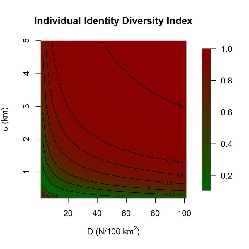
bioRxiv preprint first posted online Feb. 15, 2018; doi: http://dx.doi.org/10.1101/265678. The copyright holder for this preprint
 (which was not peer-reviewed) is the author/funder, who has granted bioRxiv a license to display the preprint in perpetuity.
                              It is made available under a CC-BY-NC-ND 4.0 International license.

   e.g., σ for the common half-normal detection model. Note, however, that the key feature
   that both population density and home range size determine which is directly responsible for
   the magnitude of uncertainty in individual identity is the magnitude of home range overlap,
   or more conceptually, the magnitude of overlap in individual utilization distributions (e.g.,
   as quantified by Fieberg & Kochanny, 2005), which increases independently by increasing
   either population density or home range size.
        We propose a metric to quantify the degree of home range overlap for a given population
   density and σ, and thus, the expected magnitude of uncertainty in individual identity. The
   Simpson’s Diversity Index can be applied to the individual detection probabilities averaged
   over many points on the landscape and realizations of the SCR process model to produce
   an Identity Diversity Index (IDI), which is conceptually similar to a metric of utilization
   distribution overlap for all individuals in the population. The details of how to calculate
   the proposed IDI can be found in Appendix A, but Figure 1 provides a visualization of how
   the magnitude of uncertainty in individual identity scales with population density and home
   range size as quantified by the SCR σ parameter. This relationship between the magnitude of
   uncertainty in individual identity and the spatial features of animal populations are what set
   a SPIM apart from the recently introduced non-spatial partial identity models (e.g. Bonner
   & Holmberg, 2013; McClintock et al., 2013; Knapp et al., 2009), where the magnitude of
   uncertainty in individual identity scales with population abundance alone.
        Another key feature of the currently available SPIM models is that partial identity in-
   formation can reduce the uncertainty in individual identity through three mechanisms–by
   adding deterministic identity associations, adding deterministic identity exclusions, and by
   improving probabilistic identity associations. Here, we define a deterministic identity asso-
   ciation as a connection between samples from the same individual that also implies that the
   samples are excluded from being connected with samples from other individuals. This is
   distinguished from a deterministic identity exclusion, which can only prevent certain sam-
   ples from being combined together. A probabilistic identity association occurs when two
   samples have a positive posterior probability of belonging to the same individual, and as
   this probability increases, the probability they belong to another individual necessarily de-
   creases. Probabilistic identity associations can be improved with partial identity information,

                                                                       5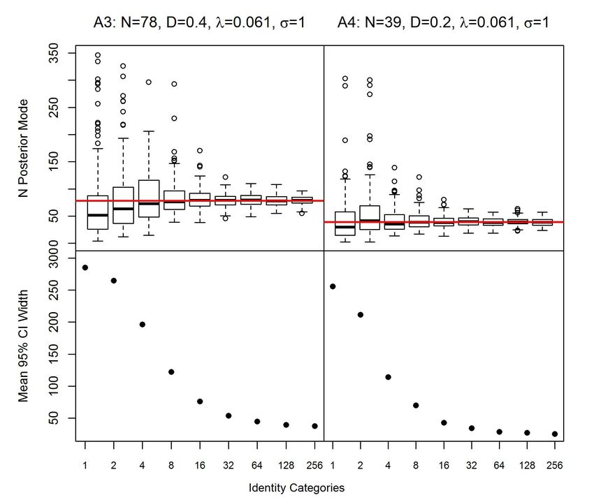
bioRxiv preprint first posted online Feb. 15, 2018; doi: http://dx.doi.org/10.1101/265678. The copyright holder for this preprint
 (which was not peer-reviewed) is the author/funder, who has granted bioRxiv a license to display the preprint in perpetuity.
                              It is made available under a CC-BY-NC-ND 4.0 International license.

   effectively converging to deterministic identity associations as partial identity information
   increases.
        All SPIM models use the spatial location where samples were collected to improve prob-
   abilistic identity associations. The unmarked SCR (Chandler & Royle, 2013) uses this in-
   formation alone to inform individual identity. Typical SCR, on the other hand, uses all
   possible deterministic identity associations. SMR (Sollmann et al., 2013) and the 2-flank
   SPIM (Augustine et al., in press) represent two intermediate cases that both utilize some
   deterministic identity associations and exclusions. SMR makes deterministic identity as-
   sociations between the samples of identifiable individuals, usually marked, but potentially
   unmarked, which simultaneously excludes them from being connected to samples from other
   individuals. Deterministic identity exclusions are then made between the samples of uniden-
   tifiable individuals whose mark status can be observed (e.g., an unmarked sample cannot
   belong to a marked individual Royle et al., 2013). The 2-flank SPIM makes deterministic
   identity associations across the same flank of the same individual, enforcing exclusions with
   non-matching samples from the same flank. Deterministic identity exclusions arise in the
   2-flank SPIM from the fact that an individual can only have one left and right flank.
        Augustine et al. (in press) demonstrated that further deterministic identity exclusions
   are possible in SPIMs by using individual sex to split a data set into two population groups
   whose latent identities could not logically match, reducing the uncertainty in individual
   identity and thus abundance and density estimates. Splitting the population into identity
   subgroups of increasingly smaller size is conceptually similar to applying unmarked SCR to
   separate populations, each with increasingly lower population densities, moving the popula-
   tion under study to more favorable regions of the IDI along the density dimension (Figure
   1). However, rather than splitting data sets into increasingly small subsets, it is desirable
   to have a model that incorporates these categorical identity exclusions, allows for imperfect
   observation of the category levels, and allows parameters to be shared across population
   identity subgroups. Further, when all categories are combined into a single analysis, the
   distribution of individuals across the category levels provides further information that can
   improve the probabilistic identity associations. For example, if a population is 75% female,
   it is more likely that two nearby male samples came from a single individual than if the

                                                                       6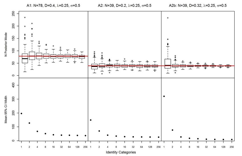
bioRxiv preprint first posted online Feb. 15, 2018; doi: http://dx.doi.org/10.1101/265678. The copyright holder for this preprint
 (which was not peer-reviewed) is the author/funder, who has granted bioRxiv a license to display the preprint in perpetuity.
                              It is made available under a CC-BY-NC-ND 4.0 International license.

   population is 75% male. Thus, we are introducing a new class of SCR model, the “cate-
   gorical SPIM”, which uses partially identifying identity covariates to add both deterministic
   identity exclusions and reduce the uncertainty in probabilistic identity associations.
        Partially-identifying categorical covariates exist in many types of invasive and noninva-
   sive wildlife sampling; for example, in studies using remote cameras, features such as sex,
   age class, and color morph may be observable in at least some photographs. In more invasive
   wildlife sampling involving live capture, many more features are measurable and researchers
   may apply categorical marks whose combination do not provide full identities (e.g., colored
   collars or ear tags), or categorical marks may be fully identifying (e.g., Lewis et al., 2015), but
   imperfectly observed. Perhaps the most informative source of categorical identity covariates
   come from microsatellite genotypes, which we will use as the main application to demon-
   strate how the categorical and spatial information combine to determine the magnitude of
   uncertainty in individual identity.
        In genetic mark-recapture, individual identities are constructed from amplified microsatel-
   lite loci – non-coding, highly variable segments of the genome–with individuals considered
   individually unique when a sufficient number of loci are amplified that it is very unlikely that
   any two individuals in the population share the same multilocus genotype. The number of
   loci necessary to guarantee uniqueness of all genotypes in a population with near certainty
   depends on the diversity of genotypes and the genotype frequencies at each microsatellite
   loci (Waits et al., 2001). This determination is typically made using P(ID) and/or P(sib) cri-
   teria, both of which estimate the probability that any two randomly selected individuals (or
   full siblings) in a population would share the same multilocus genotype given the observed
   allele diversities and frequencies (Waits et al., 2001).
        The standard practice in genetic capture-recapture is to use enough microsatellite loci
   such that P(ID) or P(sib) are less than a strict threshold, such as 0.05 or 0.01. Although
   this approach can effectively minimize the number of individuals erroneously classified as the
   same individual in a capture-recapture data set, these errors cannot be completely eliminated
   with absolute certainty. The possibility that multiple individuals have the same multilocus
   genotype in a capture-recapture data set has been referred to as the “shadow effect” (Mills
   et al., 2000) and is considered a type of low-frequency error in assigning individual identities

                                                                       7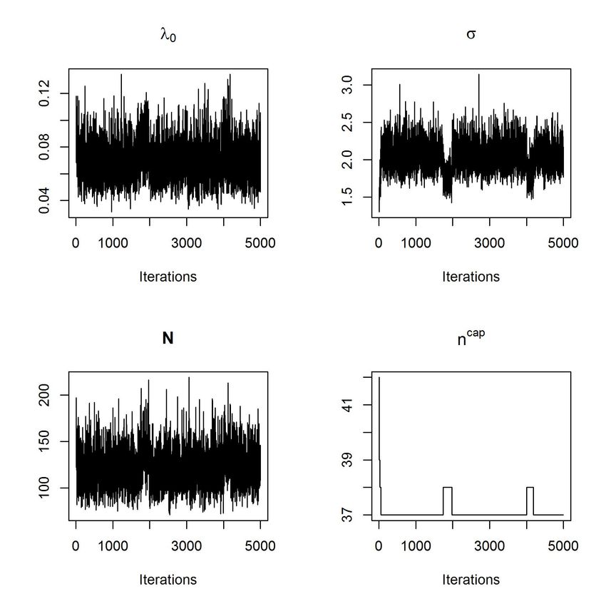
bioRxiv preprint first posted online Feb. 15, 2018; doi: http://dx.doi.org/10.1101/265678. The copyright holder for this preprint
 (which was not peer-reviewed) is the author/funder, who has granted bioRxiv a license to display the preprint in perpetuity.
                              It is made available under a CC-BY-NC-ND 4.0 International license.

   that introduces minimal bias into parameter estimates in capture-recapture studies as long as
   P(ID) or P(sib) criteria are strictly enforced. Using the categorical SPIM to model genotype
   data is especially appealing as it does not make deterministic connections between samples
   with matching genotypes and thus, multiple individuals in the population may have the
   same genotype, shifting the “shadow effect” from a source of bias to an additional source of
   uncertainty.
        Here, we generalize the unmarked SCR model to develop the “categorical SPIM”. We
   show via simulation that in scenarios with more sparse data than previously considered
   and/or scenarios with larger sigmas and larger densities, the unmarked SCR density estima-
   tor is biased and very imprecise, demonstrating the importance of population density and
   home range size to the application of latent and partial identity SCR models. We then show
   that adding categorical identity covariates removes this bias and increases precision, allowing
   for reliable density estimation across a wider range of values of density and σ for a given cap-
   ture process scenario. We also demonstrate that the uncertainty in the posterior for ncap , the
   latent number of individuals captured during a survey, correlates well with the uncertainty in
   the posterior of N , suggesting it is a good single metric to quantify the observed magnitude
   of uncertainty in individual identity for a given survey. Finally, we apply the categorical
   SPIM to a previously-published black bear data set in which we demonstrate how well the
   proposed model can reproduce the original density estimate using fewer loci than originally
   genotyped. Using this data set, we demonstrate that all uncertainty in individual identity
   can be removed with enough categorical identity covariates, producing equivalent estimates
   to an SCR model where all identities are known with certainty.

   2        Methods – Data and Model Description

   2.1        Methods – Unmarked SCR Foundation

   First, we introduce the version of the unmarked SCR model that we will expand to allow
   categorical identity covariates. The unmarked SCR model is a typical hierarchical SCR model
   except that information about individual identity is not retained during the observation

                                                                       8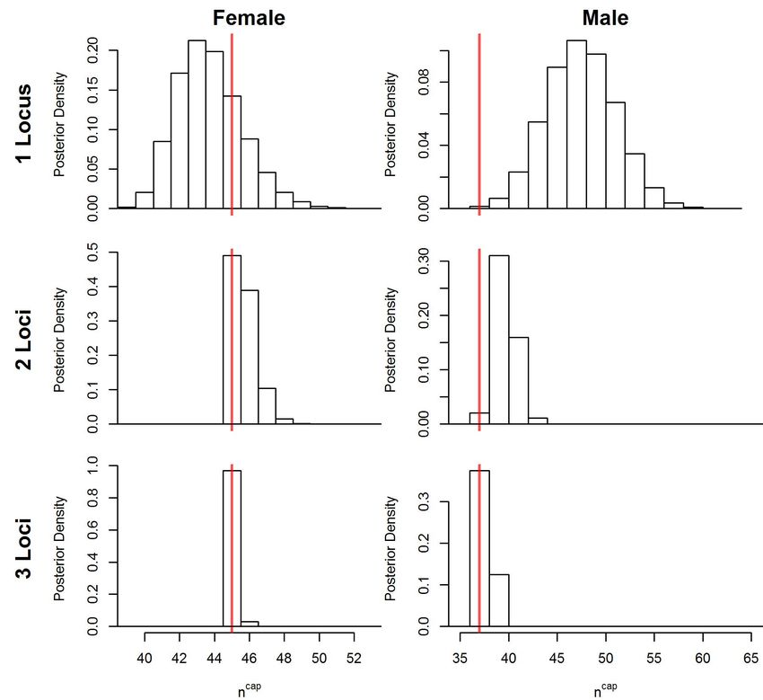
bioRxiv preprint first posted online Feb. 15, 2018; doi: http://dx.doi.org/10.1101/265678. The copyright holder for this preprint
 (which was not peer-reviewed) is the author/funder, who has granted bioRxiv a license to display the preprint in perpetuity.
                              It is made available under a CC-BY-NC-ND 4.0 International license.

   process. Formal inference is achieved by relating the spatial pattern of observed counts or
   detections at each of the J traps to the latent structure of the SCR process model. For the
   process model, we assume the N individuals in the population have 2-dimensional activity
   centers that are distributed uniformly across a two-dimensional state space S of arbitrary
   size (A) and shape, i.e. si ∼ Uniform(S), i = 1, . . . , N (see Borchers & Efford, 2008; Reich
   & Gardner, 2014; Royle et al., 2016, for alternative specifications). The activity centers are
   organized in the N × 2 matrix S.
        For the observation model, we introduce the N × J fully latent capture history Y true ,
   recording the number of detections or counts for each individual at each trap summed across
   the K occasions. The locations of the J traps are stored in the J × 2 matrix X. We assume
   that the number of counts or detections for each individual at each trap is a decreasing func-
   tion of distance between the activity centers and traps. If using a count model, we assume the

                                                                                        ||s −x ||2
   latent counts are Poisson: yijtrue ∼ Pois(Kλ(si , xj )), where λ(si , xj ) = λ0 exp − i2σ2j       ,
   xj is the location of trap j, λ0 is the expected number of counts for a trap located at distance
   0 from an activity center, and σ is the spatial scale parameter determining how quickly the
   expected counts decline with distance. We also consider an alternative Bernoulli observation
   model for which yijtrue ∼ Bin(p(si , xj ), K), where p(si , xj ) = 1 − exp(−λ(si , xj )).
        During the observation process, the true, latent capture history, Y true , is disaggregated
   into the observed capture history, Y obs , discarding information about individual identity by
   storing one observation per row in Y obs (e.g., no samples are deterministically connected
   to the same individual). More specifically, Y obs is the nobs × J matrix with entries 1 if
   sample m was recorded in trap j and 0 otherwise. Note that if we assume a Bernoulli
   observation model, each detection event will constitute a single observation, while if we
   assume a Poisson observation model, counts are disaggregated into observations of single
   counts, because counts from the same individuals cannot be deterministically connected
   without certain and unique identities. To visualize this, below is an example of true and

                                                                       9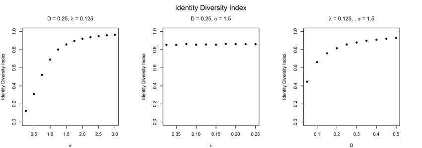
bioRxiv preprint first posted online Feb. 15, 2018; doi: http://dx.doi.org/10.1101/265678. The copyright holder for this preprint
(which was not peer-reviewed) is the author/funder, who has granted bioRxiv a license to display the preprint in perpetuity.
It is made available under a CC-BY-NC-ND 4.0 International license.
disaggregated observed data set where N =2 and J=3:
1 0 0
2 0 0 1 0 0
Y true = Y obs =
0 1 1 0 1 0
0 0 1
2.2 Methods – Categorical SPIM
We propose a class-structured version of the unmarked SCR model in which class membership
is determined by each individual’s full categorical identity (e.g., full genotype). Here, we
define a full categorical identity to be an individual’s set of true values for ncat categorical
covariates, where ncat is the maximum number of categorical covariates considered, and
multiple individuals in the population can share the same full categorical identity. We will
modify this model such that single or multiple categorical covariates, potentially partially
or even fully unobserved, are recorded with each observed sample at each trap. Further,
continuous covariates could be discretized into categories if it is safe to assume there is
no measurement error. The linked density and categorical covariate models (joint process
model) are fully latent and we use the nobs trap-referenced, observed categorical covariates
to make inference about this latent structure. The observed data then consist of two linked
data structures: Y obs , an nobs × J capture history indicating the trap at which each sample
was recorded and Gobs , an nobs × ncat identity history recording the observed categorical
covariate(s) of each sample with category level enumerated sequentially as described below,
or recorded as a 0 if not observed.
For the joint process model, we assume that each individual has a full categorical identity
associated with its activity center. Following Wright et al. (2009), we assume that all possible
category levels for each categorical covariate are known, with the number of categories for
each covariate l being nlevels
l , l = 1, . . . , ncat . Next, we introduce the population category level
probabilities for category l, γl , of length nlevels
l and corresponding to the enumerated category
levels (1, . . . , nlevels
l ) for covariate l. Then we introduce the N ×ncat matrix Gtrue , where gitrue
is the full categorical identity of the individual with activity center si . Finally, we assume
10bioRxiv preprint first posted online Feb. 15, 2018; doi: http://dx.doi.org/10.1101/265678. The copyright holder for this preprint
(which was not peer-reviewed) is the author/funder, who has granted bioRxiv a license to display the preprint in perpetuity.
It is made available under a CC-BY-NC-ND 4.0 International license.
the categorical identity of each individual for each covariate are distributed following the
covariate-specific category level probabilities according to giltrue ∼ Categorical(γl ), implying
that category levels are independent across covariates (e.g., linkage equilibrium in the genetic
context) and individuals. Using the example true and observed capture histories above,
potential true and observed structures for the categorical identities are:
1 8 3
1 8 3 1 8 3
Gtrue = Gobs =
4 2 3 4 0 3
0 0 3
In this case, the first two observed samples could possibly have come from the same individual
as could the third and fourth sample; however, the third sample could not have come from the
same individual as the first two samples. The fourth sample with two unobserved categories
could possibly belong to the same individual as that which produced the first three samples,
with only the third sample being a correct match.
The observation process is the same as unmarked SCR except that a categorical identity,
potentially partially or fully latent, is associated with each trap-referenced observation. The
missing data process could be a simple binomial model for identification success, perhaps
with covariate-specific identification probabilities; however, if we assume that covariate ob-
servation values do not vary by individual or by category level, the likelihood for the missing
data process does not change when updating latent identities or latent categorical covariate
values and can be ignored in the MCMC algorithm. Therefore, we will make the assump-
tion that covariate identification probabilities do not vary by individual or category level;
however, this assumption would be easy to relax.
The unmarked SCR model and categorical SPIM use a process similar to data augmen-
tation to estimate population abundance and density (Royle et al., 2007) and to model the
uncertainty in individual identity by providing latent structure to allow for different configu-
rations of the observed samples across the individuals in the population (Chandler & Royle,
2013; Augustine et al., in press). Unlike typical data augmentation, the number of captured
individuals, ncap , in unmarked SCR is unknown, so rather than augmenting the observed
11bioRxiv preprint first posted online Feb. 15, 2018; doi: http://dx.doi.org/10.1101/265678. The copyright holder for this preprint
(which was not peer-reviewed) is the author/funder, who has granted bioRxiv a license to display the preprint in perpetuity.
It is made available under a CC-BY-NC-ND 4.0 International license.
capture history, a fully latent capture history, Y true , of size M × J is defined and Y true is
initialized by assigning the observed samples in Y obs an individual identity based on the
spatial proximity of samples and the compatiblity of their observed categorical identities.
We then augment Gtrue to size M × ncat , which is initialized using the minimally-implied
categorical identity of the samples each individual is initialized with and the remaining
elements of Gtrue that are not determined by these samples are simulated from the category
level probabilities. Similar to typical data augmentation, M is chosen by the analyst to be
much larger than N and we use z, a latent indicator vector of length M , to indicate which
individuals are in the population; however, unlike typical data augmentation, this vector is
fully, rather than partially latent. We assume zi ∼ Bernoulli(φ), inducing the relationship
N ∼ Binomial(M, φ). Then population abundance is N = M
P
i=1 zi and population density,
N
D, is A
. See Appendix B for a full description of the MCMC algorithm.
Note that ncap , the total number of individuals captured, typically denoted by n and
a known statistic in capture-recapture models, is a derived, random variable in unmarked
SCR with a posterior distribution that quantifies the magnitude of uncertainty in individual
identity. As more categorical identity information is added, the posterior distribution of ncap
should converge to the single, true value. Finally, we introduce the derived vector, I, of size
nobs , that records the latent individual, 1, . . . , M , each sample is assigned to. This vector is
updated on each MCMC iteration, producing a posterior for true identity for each sample
which can be post-processed to obtain pairwise posterior probabilities that any two samples
originated from the same individual. The posterior distribution of the true covariate values
of samples with missing values can also be recorded.
3 Simulations
3.1 Simulation Specifications
We conducted two simulation studies to explore the performance of the categorical SPIM.
First, we conducted a simulation study to demonstrate that adding an increasing number
of identity categories removes bias from the unmarked SCR density estimator and increases
12bioRxiv preprint first posted online Feb. 15, 2018; doi: http://dx.doi.org/10.1101/265678. The copyright holder for this preprint
(which was not peer-reviewed) is the author/funder, who has granted bioRxiv a license to display the preprint in perpetuity.
It is made available under a CC-BY-NC-ND 4.0 International license.
accuracy and precision. Here, the number of identity categories is defined to be the total
number of unique categories implied by the ncat covariates with nlevels
l each. These simu-
lations were also constructed to demonstrate that the performance of unmarked SCR and
the effectiveness of adding identity categories varies as a function of population abundance,
density given abundance, and σ.
We start with the sampling scenario similar to that of Chandler & Royle (2013); however,
we make two modifications to create scenarios more challenging for the unmarked SCR
estimator. Chandler & Royle (2013) explored a range of optimistic sampling scenarios as a
proof of concept for the unmarked SCR estimator, where sampling takes place on a 15 x 15
trapping array with unit spacing within a 20 x 20 state space, λ0 = 0.5, σ ∈ {0.5, 0.75, 1},
and D ∈ {0.0675, 0.1125, 0.1875}, corresponding to N ∈ {27, 45, 75}. We consider scenarios
with higher D given N , achieved by decreasing the size of the trapping array and state
space, and with more sparse detection data. We increased data sparsity by reducing λ0 to
0.25 for the first two scenarios and further for the subsequent two scenarios (see below),
and reducing the number of traps by 64% from 225 to 81 (9 x 9 grid with unit spacing,
buffered by 3 units). We considered higher densities for similar values of N by specifying
D ∈ {0.17, 0.35}, corresponding to N ∈ {39, 78} the latter D being larger than explored
by Chandler & Royle (2013) for a similar N (75). We considered that the populations were
sampled for K = 10 occasions (Chandler & Royle, 2013, considered K ∈ (5, 10)).
We conducted simulations across 4 scenarios with a 2 x 2 factorial design using low and
high values of σ and D. Scenarios A1 and A2 were the low σ scenarios with σ = 0.5,
and Scenarios A3 and A4 doubled σ to 1. To account for compensation in the detection
function parameters (Efford & Mowat, 2014) and maintain similar levels of data sparsity
with the larger σ, we lowered λ0 from 0.25 to 0.061 to approximately match the expected
number of captures for each individual to that of the scenarios with σ = 0.5 (E[caps]≈1.65,
achieved by trial and error). On this unit spacing grid, with σ = 0.5, the majority of
an individual’s captures fell within a 4-trap area, whereas with σ = 1 the majority of an
individual’s captures fell within a 16-trap area. Scenarios A1 and A3 were the high abundance
scenarios with N=78, and Scenarios A2 and A4 were the low abundance scenarios with N=39.
The approximate Identity Diversity Indices (interpolated from Figure 1) for scenarios A1-
13bioRxiv preprint first posted online Feb. 15, 2018; doi: http://dx.doi.org/10.1101/265678. The copyright holder for this preprint
(which was not peer-reviewed) is the author/funder, who has granted bioRxiv a license to display the preprint in perpetuity.
It is made available under a CC-BY-NC-ND 4.0 International license.
A4 were 0.38, 0.23, 0.76, 0.58. Within each scenario, we explored 9 subscenarios with
differing numbers of identity categories, with 1 identity category corresponding to unmarked
SCR. Following the unmarked SCR subscenario, we sequentially added identity covariates
with 2 category levels each, leading to the number of unique identity categories increasing
exponentially with base 2 (2, 4, 8, 16, 32, 64, 128, 256).
Further, scenario A2 was modified to better disentangle the effects of increasing D from
increasing N . Increasing D by increasing N simultaneously increases uncertainty in individ-
ual identity and reduces data sparsity, which have opposite effects on estimator precision.
Therefore, to better explore the effect of increasing D has on the uncertainty in individual
identity, D must be increased by constraining a fixed N into a smaller state space. The state
space can be reduced in two ways; the number of traps can be reduced, keeping the same
state space buffer, or the number of traps can be fixed, reducing the state space buffer. In
the first scenario, data sparsity is increased since a lower proportion of individuals will be
located on the interior of the trapping array and we suspect the absolute number of traps
is important for unmarked SCR density estimation. In the second scenario, data sparsity
is decreased because a larger proportion of individuals live on the interior of the trapping
array. In order to retain the same number of traps, we chose to increased the density of
scenario A2 by reducing the state space buffer from 3 to 1 units, thus constrainting the N
individuals into a reduced state space area (Scenario A2b). The reduction in the state space
area increased D from 0.17 to 0.32, and raising the approximate IDI value from 0.23 to 0.37.
We conducted a second simulation study to demonstrate that the categorical SPIM can
accommodate partially-observed categorical identities and provide a proof of concept for
using partial genotypes that are the result of failed DNA amplification, rather than as part
of the study design as would be the case in the first set of simulations if identity categories
were genotype loci. We used the parameter values from scenario A3 above, but introduced
imperfect detection to the observed genotypes. We simulated data sets with 7 categorical
identity covariates, each with 5 equally common category levels, and the category value for
each categorical covariate was then observed with probability 0.5, leading to the average
categorical identity being observed at 3.5 of the categorical identity covariates. We fit the
categorical SPIM model to these data sets, assuming all partial categorical identities were
14bioRxiv preprint first posted online Feb. 15, 2018; doi: http://dx.doi.org/10.1101/265678. The copyright holder for this preprint
(which was not peer-reviewed) is the author/funder, who has granted bioRxiv a license to display the preprint in perpetuity.
It is made available under a CC-BY-NC-ND 4.0 International license.
usable (Scenario B1) or 75% of the partial categorical identities were usable as might be
the case when using partial genotypes if a subset was deemed to be unreliable due to the
likelihood of containing genotyping errors (Scenario B2). We then fit the null SCR model to
the perfectly observed data for comparison (Scenario B3).
For simulation scenarios A, we simulated and fit our model to 144 data sets within each
subscenario, and for simulation scenarios B, we simulated and fit our model to 128 data
sets (due to cluster computing availability). We ran single MCMC chains starting from the
simulated parameter values for 60,000 iterations, enough to produce effective sample sizes
for abundance of 400 or more for the categorical SPIM scenarios with 2 or more identity
categories. The mixing for most unmarked SCR scenarios with 1 identity category was very
poor for these challenging scenarios and frequentist performance was unlikely to improve with
longer chains. We calculated point estimates using the posterior mode and interval estimates
using the highest posterior density (HPD) interval. We were interested in the frequentist
bias and coverage of the categorical SPIM estimator, the accuracy of the estimator depicted
visually by the variance and right skew of the sampling distribution and quantitatively by
the mean squared error and coefficient of variation (100×posterior sd/posterior mode), and
the precision, quantified by the mean 95% HPD interval width. Also of interest was the use
of the precision of ncap , also quantified by the mean 95% HPD interval width, as a metric of
uncertainty in the individual identity of observed samples that can predict the uncertainty
in N .
3.2 Simulation Results
The unmarked SCR abundance estimator was right-skewed with high variance (Figures 2 and
3), except in Scenario A2 where both σ was small and abundance was low. The unmarked
SCR estimator had a large mean 95% CI width relative to abundance in all scenarios. The
unmarked SCR abundance estimates were negatively biased (Table B1; Appendix B) in
the higher abundance scenarios (A1 and A3) and positively biased in the lower abundance
scenario with the larger σ (A4) or larger density (A2b). Adding and increasing the number
of identity categories reduced bias and increased precision in all scenarios; however, with
diminishing returns as more identity categories were added. The reduction in mean 95% CI
15bioRxiv preprint first posted online Feb. 15, 2018; doi: http://dx.doi.org/10.1101/265678. The copyright holder for this preprint
(which was not peer-reviewed) is the author/funder, who has granted bioRxiv a license to display the preprint in perpetuity.
It is made available under a CC-BY-NC-ND 4.0 International license.
width for ncap by the introduction of identity categories was closely related to the reduction
in mean 95% CI width for abundance; however, the relationship was not linear and varied by
scenario (Figure 4). More identity categories were required to reach maximum precision when
abundance was higher and σ larger. The largest improvement in precision and abundance
with the addition of identity categories was seen in the low abundance, high density, low
σ scenario (A2b), where the majority of uncertainty in abundance was removed with the
addition of 1 2-level categorical covariate. Note that the precision of A2b converged to a
lower value than scenario A2 because the same N = 39 individuals were constrained to be
located within 1 unit of the trapping array, rather than 3 units, decreasing data sparsity.
Adding just a few identity categories changed the negative bias in abundance for the high
abundance scenarios to positive bias, and magnified the positive bias in the low abundance
scenarios, a pattern that was more pronounced in the large σ scenarios and which we dis-
cussed further in the application. However, this positive bias was removed by the addition of
more identity categories. Positive bias in N̂ wasbioRxiv preprint first posted online Feb. 15, 2018; doi: http://dx.doi.org/10.1101/265678. The copyright holder for this preprint
(which was not peer-reviewed) is the author/funder, who has granted bioRxiv a license to display the preprint in perpetuity.
It is made available under a CC-BY-NC-ND 4.0 International license.
nearly as precise as the scenario in which the identities were perfectly observed (Table 1). In
these scenarios, categorical identities were observed at half of the 7 identity covariates, on
average, producing data sets with an average of less than 1 sample observed at all category
levels–data sets that would be unusable if full categorical identities were required, as might
be the case with genetic capture-recapture. In Scenario B1, where all partial categorical
identities were used, the interval estimate was 95% as precise as the complete data analysis,
and in Scenario B2, where 25% of the partial categorical identities were unusable, the interval
estimate was 80% as precise than the complete data analysis. In both scenarios, an average
of 3.5 categorical covariates provided enough information that the uncertainty in ncap was
small (mean credible interval widths of 1.8 and 2.4 relative to mean ncap of 18.5 and 17.0 in
B1 and B2, respectively).
4 Application – Central Appalachian Black Bears
We applied the categorical SPIM model to an American black bear noninvasive hair trapping
data set that used 7 microsatellite loci for individual identification. This data set comes from
a study conducted along the Kentucky-Virginia, USA border across 2 study areas during
2012 and 2013 to estimate the population density and abundance of a recently reintroduced
population that was in the process of recolonizing vacant range (Murphy et al., 2016). We
chose to use the data set from the larger study area in 2013 because our model should
perform better on the larger trapping array and more samples were collected in 2013 than
in 2012 at this site. The specifics of the data collection methods are described by Murphy
et al. (2016); of particular relevance is that eighty-one hair traps were deployed across the
215-km2 study area with an average trap spacing of 1.6 km, and all traps were checked
weekly for 8 consecutive weeks, with a week constituting a capture occasion. Similar to
most bear hair trapping studies, hair samples were subsampled for genotyping because of
the prohibitive costs of genotyping thousands of samples, such that at most 1 hair sample per
trap per occasion produced an individual identity. The capture and subsampling processes
resulted in 95 samples from 45 females and 87 samples from 37 males, determined using the
P(sib) criterion. The spatial distribution of traps and individually-identified hair sample
17bioRxiv preprint first posted online Feb. 15, 2018; doi: http://dx.doi.org/10.1101/265678. The copyright holder for this preprint
(which was not peer-reviewed) is the author/funder, who has granted bioRxiv a license to display the preprint in perpetuity.
It is made available under a CC-BY-NC-ND 4.0 International license.
observations are depicted in Figure 5. The microsatellites used were G10H, G10L, G10M,
MU23, G10J, G10B, and G10P, which had genotype frequencies of 19, 22, 19, 17, 12, 15,
and 10 for females and 21, 18, 18, 22, 14, 13, and 10 for males. Despite the large number of
genotypes at each locus, the majority of individuals shared just 2-4 genotypes at each locus,
making them less informative than if the loci-specific genotypes were equally distributed as
they were in our simulation studies.
The goal of this analysis was to fit the categorical SPIM using from 1 to 7 loci, added in
the order listed above, and to compare the estimates to the null SCR estimate that does not
allow for any uncertainty in individual identity. Further, we also consider a scenario adding
partial genotype samples (2 for females, 4 for males) into the analysis that were originally
discarded. For all genotype scenarios, the trapping array was buffered in the X and Y
dimension by 3 km for females and 6 km for males, leading to state space sizes of 1042.5 km2
and 1473.4 km2 for females and males, respectively. For each sex-specific, 1-7 loci data set,
we ran 32 Markov chains for 250,000 iterations each, thinned by 50, and discarded the first
25,000 iterations as burn in, leaving 1.4 million samples from the posterior. This large number
of posterior samples was likely far more than necessary; however, it allowed us to explore the
behavior of the MCMC chains as the last uncertainty in ncap was removed by adding genotype
information (see Supplement 1). Because the hair sample subsampling process allowed for
at most 1 sample per individual/trap/occasion, we used a Bernoulli observation model.
The metrics of comparison were the point estimates (posterior modes), posterior standard
deviations, and coefficients of variation (100×posterior sd/posterior mode) for abundance
as well as the posterior distributions of ncap . Note, however, that the analyses adding the
partial genotypes should not be expected to reproduce the null SCR point estimates, standard
deviations, and number of individuals captured because they included additional data not
used by the null SCR estimate.
4.1 Application – Results
The categorical SPIM estimates (Table 2) for both sexes generally demonstrated the same
patterns seen in the simulations. Abundance estimates with few identity categories were
positively biased (relative to the SCR estimate) because the estimates of σ were negatively
18bioRxiv preprint first posted online Feb. 15, 2018; doi: http://dx.doi.org/10.1101/265678. The copyright holder for this preprint
(which was not peer-reviewed) is the author/funder, who has granted bioRxiv a license to display the preprint in perpetuity.
It is made available under a CC-BY-NC-ND 4.0 International license.
biased and/or the estimates of ncap were positively biased. The magnitude of bias was larger
for males, either partially or fully the result of a larger σ, estimated to be 2 times larger than
females; although. As more loci were added, the categorical SPIM abundance estimates
and their posterior standard deviations converged towards those of the SCR model and
the posterior modes of ncap converged towards the true number captured and the posterior
variance of ncap converged towards 0 (Figure 6). The coefficient of variation for all categorical
SPIM estimates was lower than 0.20, except for the 1 loci male estimate.
The 1 locus female estimate was only 30% percent less precise than the full SCR es-
timate, with a positive bias (relative to the complete data estimate) of 7.5%. The 3 loci
female estimate was substantially better–11.5% less precise than the full SCR estimate and
positively biased by only 2.5%. The 4 loci female estimate was effectively equivalent to the
full SCR estimate, with 3% less precision and minimal bias. The 5-7 loci female estimates
were negligibly improved. Adding 2 partial genotype samples reduced the posterior standard
deviation by 1.7% and coefficient of variation less than 1%. One partial genotype sample
was consistent with two different individuals in the full genotype data set, matching one with
posterior probability of 0.452 and the other with posterior probability 0.544, leaving just a
0.004 posterior probability that this sample was from a new individual. The other partial
genotype matched an individual with 2 captures in the full genotype data set with posterior
probability 0.997, leaving a probability of 0.003 that this was a new individual, and adding
a high probability spatial recapture for this individual.
The 1 locus male estimate was too biased (relative to the full SCR analysis) and imprecise
to be of use, whereas the 2 and 3 loci male estimates had reasonable precision but perhaps
too much positive bias to be useful. The 4 loci male estimate was 17% less precise than
the full SCR estimate, with a positive bias of 7.7%. The 5 loci estimate is only negligibly
less precise than the full SCR estimate, and adding the 6th and 7th loci improved precision
negligibly. Adding 4 partial genotype samples modestly increased the abundance estimate,
increased the posterior standard deviation (due to the larger point estimate), and decreased
the coefficient of variation by 2.5%. The posterior probability that three of the partial
genotype samples each came from separate individuals not represented in the full genotype
data set was 1, while the fourth partial genotype sample matched with 8 other samples from
19bioRxiv preprint first posted online Feb. 15, 2018; doi: http://dx.doi.org/10.1101/265678. The copyright holder for this preprint
(which was not peer-reviewed) is the author/funder, who has granted bioRxiv a license to display the preprint in perpetuity.
It is made available under a CC-BY-NC-ND 4.0 International license.
1 individual, each with posterior probability 1.
4.2 Application – Discussion
This analysis demonstrates that the categorical SPIM estimator performed similarly on a
real world data set as it did for simulated data; however, the positive bias in the male
estimates with few loci was larger than seen in the simulated data sets. We suspect individual
heterogeneity in detection function parameters, particularly σ, may have been present in the
male bear data set. If so, this could have led to poorer performance with few loci/identity
categories, and the requirement of more loci/identity categories to remove bias and increase
precision than if there were no individual heterogeneity. The distribution of observed spatial
recaptures in Figure 5 does seem to suggest individual heterogeneity in σ for males, with
one particular individual having a very long-distance spatial recapture and many individuals
having no spatial recaptures. The samples for this individual were rarely combined into one
individual until 3 loci were used and as ncap = 37 (the correct number of capture males)
became increasingly probable with the addition of more loci at which point, the estimate of σ
converged upwards to the full SCR estimate. This behavior is consistent with the simulations
where σ is large, but is more pronounced in this data set, which could be explained by
individual heterogeneity in the detection function parameters. A second factor that tends
to split the samples from this potentially large σ individual apart is that there were several
traps between the two traps where this individual was captured and the categorical SPIM
found it unlikely that this individual would not have been captured at these traps closer
to its estimated activity center until enough categorical covariate information was available
to make it more even more unlikely that two individuals in the population had the same
multilocus genotype. The second longest spatial recapture in the male data set spans a gap
with no traps and required fewer loci to reliably link its samples together.
The posterior distributions of ncap in Figure 6 demonstrate what we believe is a source
of the positive bias in the categorical SPIM estimator. With the addition of just 2 loci
for females and 1 locus for males, all incorrect combinations of samples were ruled out by
the genotype information and the spatial distribution of the samples. However, a 1 or 2
loci genotype is not sufficient to guarantee the local uniqueness of a genotype, leading to
20bioRxiv preprint first posted online Feb. 15, 2018; doi: http://dx.doi.org/10.1101/265678. The copyright holder for this preprint
(which was not peer-reviewed) is the author/funder, who has granted bioRxiv a license to display the preprint in perpetuity.
It is made available under a CC-BY-NC-ND 4.0 International license.
a situation in which samples cannot be erroneously combined into fewer individuals than
produced them, but they can be erroneously split apart into more individuals than produced
them. Thus, in these scenarios, ncap can never take a value lower than the true value,
but rather must always be larger than the true value. We believe the identity exclusions
are removing the lower tail of the posterior distribution of ncap that would be present in
the unmarked SCR estimator, introducing positive bias, which can be removed by adding
more categorical identity information and reducing the upper tail of the posterior of ncap .
In the simulations, this occurs with the addition of just a few identity categories; however,
individual heterogeneity in detection function parameters as argued above, may require more
categorical identity information to remove the positive bias in ncap and thus N .
This analysis also demonstrated the use of genotypes that are partial as a consequence
of DNA amplification failure, with two caveats. First, there were very few usable partial
genotypes because of the DNA amplification protocol used in which samples at the same
trap/occasion were subsequently genotyped until a full genotype was obtained. This process
led to the partial genotypes matching the complete genotype individual at a particular
trap/occasion with high probability because bears usually leave multiple hair samples in
a hair snare, violating the Bernoulli observation process. Second, we assumed the partial
genotype samples did not contain any genotyping errors. Three of the 6 partial genotype
samples used matched other individuals in the population with high probability, but 3 partial
genotypes had posterior probabilities of 1 that they were new individuals. These may have
indeed been new individuals, or perhaps they did not match any other individuals because
they were corrupted. Including partial genotypes in this manner needs to be done with
caution and in consultation with a wildlife geneticist, or the categorical SPIM could be
extended to accommodate genotyping errors (e.g. Wright et al., 2009). If partial genotypes,
or even a subsample of the partial genotypes, can be deemed reliable, including them in the
analysis can increase the precision of abundance and density estimates, especially if high
probability spatial recaptures can be added, as was the case in the female bear data set.
21bioRxiv preprint first posted online Feb. 15, 2018; doi: http://dx.doi.org/10.1101/265678. The copyright holder for this preprint
(which was not peer-reviewed) is the author/funder, who has granted bioRxiv a license to display the preprint in perpetuity.
It is made available under a CC-BY-NC-ND 4.0 International license.
5 Discussion
We developed a spatial capture-recapture model for categorically marked populations that
uses any number of partially identifying categorical covariates to reduce the uncertainty in
the individual identity of latent identity samples via three mechanisms. First, any samples
that are inconsistent at any observed covariates are deterministically excluded from match-
ing. Second, as the number of identity categories created by covariates increases and as the
category level probabilities for each covariate become more equal, it is increasingly unlikely
that more than one individual locally, and in the population, will have the same full cate-
gorical identity. Third, the spatial location of the latent identity samples and the estimated
detection function scale parameter, σ, spatially restrict which samples matching at all ob-
served covariates could have been produced by the same individual. Thus, the categorical
SPIM reduces uncertainty in the individual identity of latent identity samples by providing
deterministic identity exclusions and reducing the uncertainty in probabilistic identity as-
sociations using both spatial and categorical covariate information. The categorical SPIM
simulation and MCMC functions are maintained in the SPIM R package (Augustine, 2018)
and can also be found in Supplement 2.
A specific case of categorically marked populations that is of some practical importance
is that in which individuals are marked by multilocus genotypes. In this case, each locus of
a genotype is a single categorical covariate and the categorical SPIM provides a continuous
model for genotype uniqueness. Thus, the categorical SPIM is an alternative to using the
P(ID) and P(sib) criteria currently used that allows for uncertainty in individual identity
as might be the case when fewer loci are amplified than necessary to meet probability of
identity criteria, which might occur in populations with very low genetic diversity (e.g.
McCarthy et al., 2009). The categorical SPIM also introduces the possibility of using fewer
loci than necessary to meet probability of identity criteria by design, trading some certainty
in individual identity for lower genotyping costs. Genotyping costs do not increase linearly
with the number of loci and Puckett (2017) found that variability in the number of loci used
in microsatellite studies explains very little variability in total project costs. There may
be some cost savings if using fewer loci allows for the use of fewer multiplex panels, which
22bioRxiv preprint first posted online Feb. 15, 2018; doi: http://dx.doi.org/10.1101/265678. The copyright holder for this preprint
(which was not peer-reviewed) is the author/funder, who has granted bioRxiv a license to display the preprint in perpetuity.
It is made available under a CC-BY-NC-ND 4.0 International license.
explain a moderate amount of variability in total project costs (Puckett, 2017).
Simulation scenarios A1-4 (Figures 2 and 3) show the importance of population abun-
dance, density given abundance, and σ for the accuracy and precision of the unmarked SCR
and categorical SPIM estimators. Estimates from populations with lower density given abun-
dance and smaller σs showed less bias and estimates were more precise for populations with
higher abundances, lower density given abundance, and smaller σs. More categorical iden-
tity groups were necessary to maximize precision when abundance was higher and σ larger;
however, for the scenario that raised D without raising N , the majority of precision gains
came from the addition of the first 4 identity categories. This scenario raising D without
raising N demonstrates the importance of disentangling the relationship between N and D
when assessing the performance of unmarked SCR, and SCR models with latent or partial
individual identities, more generally. Further, it suggests that categorical identity covariates
are more effective in populations where estimator uncertainty is due to a large D relative to
N , rather than a large σ.
The IDI correlated negatively with the precision and accuracy of ncap estimates. For the
scenarios that increased the IDI holding N fixed (A1 vs. A3, A2 vs. A4, A2 vs, A2b), the
IDI also correlated negatively with the accuracy and precision of N estimates. In scenarios
that increased D by increasing N (A1 vs A2, A3 vs. A4), the increase in uncertainty in ncap
was outweighed by the decrease in data sparsity and N estimates were more precise and
accurate. Our exploration of IDI values here is very limited and a larger simulation study
is necessary to determine how well this index correlates with estimator performance and to
what degree do scenarios with differing population density and σ values producing the same
index value share the same estimator performance. Our results suggest that scenarios with
differing D and σ values that produce the same IDI values will not necessarily produce the
same precision in ncap . We speculate that this is related to how the latent identity samples
interact with different densities of activity centers in the SCR process model. Specifically,
when D is large, there are necessarily more nearby individuals that a latent identity sample
can be allocated to, which increases the uncertainty in individual identity. Finally, note
that some of the largest values of the IDI may represent ecologically implausible or even
impossible scenarios since home range size generally varies inversely with density (Efford
23You can also read