Training Deep Normalizing Flow Models in Highly Incomplete Data Scenarios with Prior Regularization
←
→
Page content transcription
If your browser does not render page correctly, please read the page content below
Training Deep Normalizing Flow Models in Highly Incomplete Data Scenarios
                                                                  with Prior Regularization

                                                                                           Edgar A. Bernal
                                                                                  Rochester Data Science Consortium
                                                                                       University of Rochester
                                                                                      edgar.bernal@rochester.edu
arXiv:2104.01482v1 [cs.LG] 3 Apr 2021

                                                                 Abstract                                    interest to the learning community (e.g., audio, language,
                                                                                                             imagery and video), reliably learning the statistical prop-
                                           Deep generative frameworks including GANs and nor-                erties of a given population of data samples often requires
                                        malizing flow models have proven successful at filling in            immense amounts of training data. Recent work has em-
                                        missing values in partially observed data samples by ef-             pirically shown that, in order to continue pushing the state-
                                        fectively learning –either explicitly or implicitly– complex,        of-the-art in high-fidelity synthetic data generation, scalable
                                        high-dimensional statistical distributions. In tasks where           models able to ingest ever-growing data sources may be re-
                                        the data available for learning is only partially observed,          quired [2].
                                        however, their performance decays monotonically as a                     Some of the data requirements imposed by current deep
                                        function of the data missingness rate. In high missing data          generative models may limit their applicability in real-life
                                        rate regimes (e.g., 60% and above), it has been observed             scenarios, where available data may not be plentiful, and
                                        that state-of-the-art models tend to break down and pro-             additionally, may be noisy, or only partially observable.
                                        duce unrealistic and/or semantically inaccurate data. We             The nature of real-world data poses challenges to existing
                                        propose a novel framework to facilitate the learning of data         models, and mechanisms to overcome those challenges are
                                        distributions in high paucity scenarios that is inspired by          needed in order to further the penetration of the technology.
                                        traditional formulations of solutions to ill-posed problems.         In this paper, we focus on enabling the learning of DMGs
                                        The proposed framework naturally stems from posing the               in scenarios of high data missingness rates (e.g., 60% of en-
                                        process of learning from incomplete data as a joint opti-            tries missing per data sample and above), where the miss-
                                        mization task of the parameters of the model being learned           ingness affects both the training and the test sets. We specif-
                                        and the missing data values. The method involves enforc-             ically focus on the task of image imputation, which consists
                                        ing a prior regularization term that seamlessly integrates           in filling in missing or unobserved values without access to
                                        with objectives used to train explicit and tractable deep            fully observed images during training. Previous work on
                                        generative frameworks such as deep normalizing flow mod-             data imputation leveraging various forms of DMGs has ex-
                                        els. We demonstrate via extensive experimental validation            plicitly addressed image imputation [29, 30, 41, 55]. While
                                        that the proposed framework outperforms competing tech-              the results are reasonable in low- and mid-data missingness
                                        niques, particularly as the rate of data paucity approaches          regimes, empirical results indicate that, as large fractions of
                                        unity.                                                               the data become unobserved, either the perceived quality of
                                                                                                             the recovered data suffers [41], the original semantic con-
                                        1. Introduction                                                      tent in the image is lost [55] or both [29]. These undesired
                                                                                                             consequences are likely caused by the ill-posedness of the
                                           Deep generative models (DGMs) have enjoyed success                problem of attempting to estimate certain statistical proper-
                                        in tasks involving the estimation of statistical properties of       ties from partially observed data, an issue which becomes
                                        data. Applications of DGMs involve generation of high-               more extreme as the rate of unobserved data approaches
                                        resolution and realistic synthetic data [2, 13, 35, 38, 39],         totality. Of note, most existing work fails to consider the
                                        exact [6, 21] and approximate [22, 40] likelihood estima-            semantic content preservation aspect of the task altogether,
                                        tion, clustering [53], representation learning [1, 54], and          and focuses solely on measuring the performance of the al-
                                        unsupervised anomaly detection [23]. Fundamentally, gen-             gorithms based on the realism of the recovered data samples
                                        erative models perform explicit and/or implicit data density         [29, 30, 55].
                                        estimation [14]. Given the complexity of most signals of                 Inspired by these observations, we propose to constrain

                                                                                                         1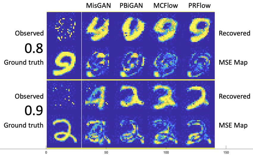
the complexity of the solution space where the recon-            Adversarial Networks (GANs) [13], including Partial VAEs
structed image lies via regularization techniques, a tech-       [32], the Missing Data Importance-Weighted Autoencoder
nique initially exploited in traditional ill-posed inverse       (MIWAE) [34], the Generative Adversarial Imputation Net-
problem formulations [49] and more recently adapted to           work (GAIN) [55] and the GAN for Missing Data (MIS-
statistical learning scenarios [51]. The proposed regulariza-    GAN) [29]. More recently, the state-of-the-art benchmark
tion term enforces a prior distribution on the gradient map      on learning from incomplete data has been pushed by bidi-
of the reconstructed images [24] in the form of a shallow,       rectional generative frameworks which leverage the ability
hand-engineered constraint, and stands in contrast with re-      to map back and forth between the data space and the la-
cent trends which rely on the high expressivity and capacity     tent space. Two such examples include the Monte-Carlo
of deep models to effectively construct data-driven priors,      Flow model (MCFlow) [41] which relies on explicit nor-
but which break down in scenarios where data scarcity is an      malizing flow models [5, 6, 21], and the Partial Bidirec-
issue. We seamlessly couple the regularizing priors with ex-     tional GAN (PBiGAN) [30] which extends the bidirectional
plicit likelihood estimates of reconstructed samples yielded     GAN framework [7, 8].
by normalizing flows in a novel framework we dub PRFlow,             While the results achieved by recent work are impres-
which stands for Prior-Regularized Normalizing Flow. The         sive in their own right, these methods share a common
contributions of this paper are as follows:                      thread: they all break down, in one way or another, as
   • a framework combining traditional explicit and              the missingness rate in the data approaches unity. This
      tractable deep generative models with shallow, hand-       phenomenon can be intuitively understood if we think of
      engineered priors in the form of regularization terms to   a generative model as a probability density estimator (ei-
      constrain the complexity of the solution space in high     ther explicit or implicit) [14], which is, at its core, an ill-
      data paucity regimes;                                      posed inverse problem [4, 43]. From this standpoint, the
   • a formal derivation of the framework stemming from          ill-posedness becomes more extreme as the rate of occur-
      the formulation of the learning task with incomplete       rence of unobserved data increases. Historically, regular-
      data as a joint optimization task of the network param-    ization techniques [9, 49] have been widely used to precon-
      eters and missing data values;                             dition estimators and avoid undesired behaviors of solutions
   • a comprehensive testing framework –including a new          by restricting the feasible space [10, 51]. While regulariza-
      metric that captures the semantic consistency between      tion in deep learning is commonplace (e.g., weight decay
      the original and the recovered data samples– which         and weight sharing [37], dropout [45], batch normalization
      evaluates all aspects of performance that are relevant     [19]), it is usually implemented to constrain the plausible
      when learning from partially observed data; and            space of network parameters and avoid overfitting in dis-
   • empirical validation of the effectiveness of the pro-       criminative scenarios. Models that implement regulariza-
      posed framework on the imputation of three stan-           tion on the output space tend to be of the generative type.
      dard image datasets and benchmarking against current       For instance, image priors have been leveraged to address
      state-of-the-art imputation models under the proposed      the inherently ill-posed single-image super resolution prob-
      testing framework.                                         lem [20, 28, 46, 52, 56]. The proposed framework can
                                                                 be seen as an attempt to incorporate domain knowledge in
2. Related Work                                                  learning scenarios in order to guide, facilitate or expedite
                                                                 the learning [11, 17, 18].
    Deep learning frameworks have proven successful at a
wide range of applications such as speech recognition, im-       3. Proposed Framework
age and video understanding, and game playing, but are
often criticized for their data-hungry nature [33]. Some             Parallels between ill-posed inverse problems and learn-
scholars go as far as to say that the future of deep learning    ing tasks have been established in the literature [42, 51].
depends on data efficiency, and have attempted to achieve        To informally illustrate how the degree of ill-posedness of
it in various ways, for example, by leveraging common            a learning task from partial observation grows with the rate
sense [48], mimicking human reasoning [12] or incorpo-           of data missingness, consider the task of image imputation.
rating domain knowledge into the learning process [36].          Let b denote the bit depth used to encode each pixel value
The ability to learn from incomplete, partially observed and     (i.e., pixels can take on values g, where 0 ≤ g ≤ 2b − 1)
noisy data will be fundamental to advance the adoption of        and N the number of pixels of the images in question. The
deep learning frameworks in real-life applications. In re-       total number of possible images that can be represented
cent years, a body of research on deep frameworks that           with this scheme is (2b )N . For the sake of discussion,
can learn from partially observed data has emerged. Ini-         let us ignore the fact that natural images actually lie on a
tial work focused on extensions of generative models such        lower-dimensional manifold within that image space. Let
as Variational Auto Encoders (VAEs) [22] and Generative          0 ≤ p ≤ 1 denote the data missingness rate. This means
that when we partially observe an image, we are only ex- of the distribution (i.e., to contrast with data-driven priors).
posed to (1 − p) · N of its pixel values. The task of image We use the notation z = x ∗ fi to denote the convolution
imputation involves estimating the remaining p · N pixel between image x and kernel fi . When multiple filters are
values, which means that for every partially observed in- used, it is common to assume independence
PI of the different
put image, there are (2b )pN possible imputed solutions. It edge maps so that log pp (x) ∝ − i=1 |x ∗ fi |α , where I
is apparent that the dimensionality of the feasible solution is the total number of filters.
space grows exponentially as the missingness rate grows In scenarios where training data is only partially ob-
linearly. The practical implication of this observation is served, training a normalizing flow model can be formu-
that, in order to maintain a certain level of reconstruction lated as a joint optimization task where two sets of parame-
performance, the number of partially observed data samples ters are learned concurrently, namely the missing entries in
needs to grow exponentially as the missingness rate grows the data and the parameters of the normalizing flow model
linearly. This is an example of an ill-posed problem where itself. Let xrec denote the reconstructed samples and Gθ the
the observed data itself is not sufficient to find unique solu- normalizing flow network parameterized by θ. The objec-
tions. tive of the learning task can be written as
When an imputation task is tackled with a learning
(xrec , θ∗ ) = arg max {p(x, θ)} (1)
framework (i.e., a deep generative network), the inductive x,θ
bias that arises from the choice of network inherently con- Note that, as per the above objective, missing data val-
straints the solution space. This restriction is not only con- ues are treated as parameters to optimize. Throughout the
venient but also necessary for learning [3], as illustrated by remainder of the paper, we will refer to these values inter-
recent work which shows that the structure of a network changeably as data parameters or missing data values.
captures natural image statistics prior to any training [50]. Estimating the joint density from Eq. 1 is difficult. One
We will demonstrate empirically that inductive bias alone way to circumvent this obstacle is to alternately optimize
is not sufficiently effective at restricting the solution space over the conditional distributions of each of the parameters
in cases where data is missing at high rates. Experimental interest, in a manner similar to the way sampling-based op-
results conclusively show that augmenting the constraining timization frameworks such as Gibbs Sampling and MCMC
properties of the inductive bias with shallow priors imple- [47] operate. Following this principle, the joint optimiza-
mented in the form of regularizers is a simple an effective tion task can be broken down into two conditional optimiza-
strategy in boosting the performance of deep models in sce- tion tasks of likelihood functions. On the one hand, learning
narios of high data paucity. the parameters θ of normalizing flow network Gθ can be
achieved in the traditional manner, that is, by maximizing
3.1. Framework Description the log-likelihood of the observed data:
Normalizing flow models are explicit generative models θ∗ = arg max {p(θ|xrec )} (2)
which perform tractable density estimation of the observed θ
data. The density estimate is constructed by learning a cas- A set of parameters θ defines an invertible network Gθ
cade of invertible transformations which perform a mapping that maps images to a tractable latent space and vice-versa.
between the data space and a latent space. A simple, con- Specifically, in order to perform log-likelihood estimation,
tinuous prior is assumed on the latent variables, for exam- a data sample xi is mapped to its latent representation yi by
ple a spherical Gaussian density. Exact log-likelihood com- passing it through Gθ , namely yi = Gθ (xi ). Since the like-
putation is achieved using the change of variable formula lihood for yi is known (e.g., from a normality assumption),
[5, 6, 21]. In this work, we introduce a principled frame- p(xi ) (i.e., the likelihood of xi ) can be computed exactly via
work that leverages the explicit and tractable likelihood ca- the variable change rule. The ability to estimate the likeli-
pabilities of normalizing flow models to impose structured hood of a data sample enables the resolution of the second
constraints on the constructed probabilistic models. conditional optimization task, which aims at finding the op-
Although the proposed framework is generic enough to timal entries for the missing values in the partially observed
support a wide range of prior constraints, this study lever- data by maximizing the likelihood of the reconstructed sam-
ages the Hyper-Laplacian prior [24], which has been proven ple conditioned on the current model parameters:
effective at modelling the heavy-tailed nature of the distri- xrec = arg max {p(x|θ∗ )} (3)
bution of gradients in natural scenes. This distribution takes x
α
on the form pp (z) ∝ e−k|z| (or equivalently, log pp (z) ∝ where the search space is constrained to images x whose
α
−k|z| ), where 0 < α ≤ 1 determines the heaviness of entries match the observed entries of xobs . Solving the opti-
the tails in the distribution, and z is the gradient map of im- mization task from Eq. 3 effectively fills in unobserved data
age x, which can be obtained by convolving x with a fam- values, that is, performs data imputation. Training the over-
ily of kernels fi . Subscript p is used to denote the nature all imputation model involves alternately solving Eqs. 2 and(n)
3, which yields a sequence of parameter pairs (xrec , θ∗(n) ). As described in Sec. 3.1, learning this framework in-
Convergence is achieved when little change is observed in volves optimizing two different objectives: training network
the updated parameters. The description of the framework Gθ and Hφ involves optimizing the objectives from Eqs. 2
around Eqs. 2 and 3 follows closely the formulation in [41], and 5 respectively, with the optimization being carried out
although in that work, the training of the model was not in an alternating way until convergence is achieved. The
framed as a joint optimization task. objectives used to learn these networks, as described below,
As stated, solving Eq. 2 involves training a traditional are denoted J (θ) and J (φ). In the context of the proposed
normalizing flow model with the current estimate of the data framework, the data parameters are not optimized directly;
parameters, i.e., the current values of the imputed data. In instead, network Hφ is learned according to J (φ), a proxy
contrast, the optimization task in Eq. 3 is a highly ill-posed objective to that in Eq. 5. We now describe how the two
problem when the data missing rate in xobs is high. PRFlow networks are learned.
leverages the key insight that regularization of the task with Learning the optimal parameters θ∗ of normalizing flow
prior knowledge on the solution space leads to improved, network Gθ is achieved by maximizing the log-likelihood
more stable solutions to Eq. 3. In order to incorporate this of the training data, or equivalently, minimizing the cost
prior knowledge, first observe that, as per the Bayes rule: function:
(n)
X
J (θ) = − log pθ (xi ) (6)
p(x|θ∗ ) ∝ p(θ∗ |x)pp (x) (4) i
where the sum is computed across training data samples,
where pp (x) is the prior introduced at the beginning of and the superscript (n) denotes samples which have been
Sec. 3.1, and it has been assumed that model parameters θ∗ imputed with the most recent (i.e., the n-th) imputation
are fixed. This is the case since at this stage in the training model. Throughout this optimization stage, the training
alternation, the optimization is over the missing data entries data remains unchanged. At initialization, where no im-
with the goal of performing data imputation. Combining putation model is available, shallow imputation techniques
Eqs. 3 and 4 and applying log yields (e.g., nearest neighbor or bilinear interpolation) are used.
Minimizing this loss corresponds to solving the optimiza-
xrec = arg max {log p(θ∗ |x) + λ log pp (x)} (5) tion task from Eqs. 2.
x
Learning the optimal parameters φ∗ of the imputation
where λ is a parameter that controls the desired degree of model, which operates in the latent space of the normaliz-
regularization. In summary, training PRFlow involves alter- ing flow network, is achieved by minimizing a three-term
nately optimizing the objectives in Eqs. 2 and 5. It is worth- loss. Updating parameters φ results in an updated imputer
while noting that the objective from Eq. 2 and the first term network Hφ , which is used to obtain an updated training set
in the objective from Eq. 5 involve optimizing the same like- x(n) . Throughout this stage, normalizing flow network Gθ
lihood function relative to two different sets of parameters, remains fixed. The first element of the loss involves max-
namely the model parameters and the missing data values, imizing the likelihood of the reconstructed samples as per
respectively. the likelihood estimate provided by the normalizing flow
model, or equivalently, minimizing the cost function:
3.2. Framework Implementation
(n)
X
PRFlow is largely based on the architecture introduced J1 (φ) = − log pθ (xi )
i
in [41], which includes a normalizing flow network G that h i (7)
(n−1)
X
enables likelihood estimation, and a network H performing =− log pθ G−1
θ ◦ Hφ ◦ Gθ (xi )
a non-linear mapping in the latent flow space and fills in i
missing values in the partially observed data samples. As where the ◦ operator denotes functional composition and
(n)
in [41], network G is an instantiation of RealNVP [6]. The the expression for xi has been expanded to emphasize
mapping to the latent space via G is performed because like- its dependence on the parameters being optimized, namely
lihood computation is tractable in that space, and the impu- φ. Minimizing this loss is equivalent to optimizing the first
tation task is being formulated as the solution of a max- term of the objective from Eq. 5. As stated before (see last
imum likelihood conditional objective (as per Eq. 3). At paragraph in Sec. 3.1), this loss is equivalent to the loss from
a high level, the imputation process comprises receiving a Eq. 6; the difference lies in the set of parameters that are be-
partially observed sample xobs , computing its latent repre- ing modified to achieve the objective. This term encourages
sentation yobs = Gθ (xobs ), mapping this latent representa- the imputer to output recovered samples that are more likely
tion to yrec = Hφ (yobs ) with maximum likelihood, and re- to occur.
covering the corresponding maximum likelihood data sam- The second element involves minimizing the discrep-
ple xrec = G−1 θ (yrec ) which matches the observed entries ancy between the recovered data and the known entries of
of xobs . This process is illustrated in Fig. 1. the observed data:Figure 1: High-level view of the imputation process.
in steps of 10%. The training procedure follows the prin-
X (n−1) ciples of recent work proposing models that support and
J2 (φ) = MSE(xi,obs , G−1
θ ◦ Hφ ◦ Gθ (xi )) (8) rely purely on partially observed data during the learning
i
phase [29, 30, 41, 55] by training with the dataset result-
where the MSE is computed across the known entries of ing from randomly dropping the corresponding percentage
the observed data only. Note that these entries remain un- of pixels from the images in the standard training set from
changed throughout both stages of the optimization process, the respective dataset of interest according to a Bernoulli
thus no superscript is needed. This term encourages the im- distribution. In MNIST, the training set comprises 60,000
puter to output recovered samples that match the known en- 28 × 28-pixel grayscale images, whereas in CIFAR it in-
tries at the observed positions. cludes 50,000 32×32-pixel RGB images. Since no standard
The last term penalizes reconstructions that deviate from partition exists for CelebA, we use the first 100,000 images
the expected behavior as dictated by the regularizing prior: for training and the remaining for testing. We pre-process
(n)
X X X (n)
J3 (φ) = − log pp (xi ) = − |xi ∗ fj |α CelebA images by performing 108 × 108 pixel center crop-
i i j ping and resizing to 32 × 32 pixels. For testing, we adhere
XX (n−1) to the experimental principle drawn out in [41], where per-
=− |G−1
θ ◦ Hφ ◦ Gθ (xi ) ∗ fj |α
formance is measured on the standard test set of the relevant
i j
dataset after having randomly dropped the appropriate frac-
(9)
tion of pixel values.
where the summations indexed by i and j are performed
Metrics. We measure the performance of the algorithms
across data samples and gradient kernels, respectively, and
relative to three different metrics, which we believe cap-
we have incorporated the expression for the prior introduced
ture all relevant attributes of data recovered by an algorithm
in Sec. 3.1. Minimizing this loss is equivalent to optimizing
attempting to reconstruct partially observed data: (i) root
the second term in the objective from Eq. 5. In our imple-
mean squared error (RMSE), which measures differences
mentation, and for the sake of computational efficiency and
between the reconstructed image and the ground truth at the
simplicity, we use two first-order derivative filters, namely
pixel level; (ii) the Fréchet Inception Distance (FID), first
[1, 1] and [1, 1]| . Note that higher-order or learnable filters
proposed to measure the quality of data produced by gener-
can be used instead, which would likely result in improved
ative models [16] and which captures population-level sim-
performance.
ilarities; and (iii) the ratio of the classification accuracy of
In summary, training PRFlow involves joint optimization
a classifier pre-trained on fully observed training data on
of objectives {J (θ), J1 (φ), J2 (φ), J3 (φ)} across θ and φ,
the reconstructed data to the accuracy of the same classi-
where θ denotes the parameters of the normalizing flow net-
fier on the fully observed test set. This metric, which we
work and φ denotes the imputer network parameters, i.e.,
denote the Semantic Consistency Criterion (SCC), aims at
the parameters that ultimately determine how the missing
measuring the amount of semantic information preserved by
data values are filled in.
the missing data recovery process. Formally, let accimp be
4. Experimental Results the performance of the benchmark classifier on an imputed
test set and acc0 the performance of the same classifier on
Datasets and Procedure. The efficacy of PRFlow the original test set. Then SCC = min{1, accimp /acc0 },
was evaluated on three different standard image datasets, where the clipping is introduced to handle the unlikely case
MNIST [27], CIFAR-10 [25] and CelebA [31]. Four differ- when accimp > acc0 . Normalization by the baseline clas-
ent rates of data missingness were tested, from 60% to 90% sifier performance is done to minimize the impact of thechoice of classifier. This overarching experimental frame- while PBiGAN performs the worst, with the gaps in per-
work contrasts with most previous work on generative mod- formance being significantly larger for CIFAR. These re-
elling of incomplete data ([41] excepted), which doesn’t sults are reasonable since neither MisGAN nor PBiGAN
consider the preservation of semantic content as a metric of enforce an MSE loss explicitly. Table 2 includes the FID
performance, and tends to make more emphasis on the real- results laid out in a similar fashion. In this case, PRFlow
ism of the recovered samples than on the pixel-level accu- again outperforms all competing methods, trailed closely
racy [29, 30]. In this work, we consider all three metrics to by PBiGAN on MNIST, with performance being more even
be equally important, and posit that one of the most salient across the field on CIFAR and CelebA. These results high-
strengths of the proposed method is that it minimizes the light the efficacy of the regularizing prior at shaping the sta-
impact of the trade-off between the metrics relative to com- tistical behavior of the recovered imagery. Lastly, Table 3
peting methods. Of note, RMSE is measured between the includes SCC results. In the MNIST case, MCFlow, PBi-
recovered values and the ground truth values at the unob- GAN and PRFlow perform similarly, with MisGAN trailing
served pixel locations in the test set. This means that not by a somewhat significant margin, and with the margin in-
only the pixels but also the full images used to measure the creasing as the missing rate increases. In the CIFAR case,
performance of the method are completely unseen by the PRFlow outperforms the competition more handily.
framework during training, unlike approaches which mea-
sure performance on unobserved values within the training Table 1: RMSE between recovered data and ground truth
set [29, 30]. Similarly, FID is measured between the recov- test set, unobserved pixels only (lower is better)
ered test set and the ground truth test set, and SCC perfor- Missing Rate
mance is measured on the recovered test set imagery. Dataset Method 0.6 0.7 0.8 0.9
MisGAN 0.1329 0.1561 0.1958 0.2484
Competing Methods. We benchmark the performance
PBiGAN 0.3155 0.3121 0.3045 0.2844
of PRFlow against three methods, namely MisGAN [29], MNIST
MCFlow 0.1126 0.1300 0.1581 0.2080
PBiGAN [30] and MCFlow [41], which together comprise PRFlow 0.1093 0.1243 0.1490 0.2059
the state-of-the-art landscape in image imputation tasks MisGAN 0.2568 0.2814 0.3081 0.3461
across the considered metrics. We used the publicly avail- PBiGAN 0.3380 0.3443 0.3623 0.4448
able code for all three competing methods from their offi- CIFAR
MCFlow 0.0921 0.1059 0.1187 0.1460
cial repositories; we used the code as published for MNIST PRFlow 0.0802 0.0919 0.1102 0.1299
and made extensions to the code to enable support of CI- MisGAN 0.2232 0.2273 0.2404 0.2777
FAR (no CIFAR versions were publicly available). We use PBiGAN 0.2894 0.3356 0.3733 0.4230
CelebA
LeNet [26], ResNet18 [15] to compute both SCC and FID MCFlow 0.0793 0.0828 0.0927 0.1189
on MNIST and CIFAR, respectively. Since CelebA has no PRFlow 0.0738 0.0813 0.0924 0.1135
classes, we use FaceNet [44] to compute FID only.
Experimental Setup. Throughout the experiments, we
use α = 1/3, a learning rate of 1 × 10⁻⁴ , and a batch size Table 2: FID between recovered data and ground truth test
of 64. We train until little change is observed in the loss sets (lower is better) Missing Rate
from Eq. 8, as opposed to competing methods which pre- Dataset Method 0.6 0.7 0.8 0.9
scribe a set number of epochs to train. Gθ is a RealNVP MisGAN 0.8300 1.5373 3.0956 7.9071
[6] network with six affine coupling layers. We implement PBiGAN 0.1356 0.3082 0.9927 4.2000
MNIST
MCFlow 0.7840 1.3382 3.0663 8.5047
Hφ as a 3-hidden layer, fully connected network with 784
PRFlow 0.0959 0.2888 0.8795 3.8759
and 1024 neurons per layer for MNIST and CIFAR/CelebA,
MisGAN 0.7299 0.8464 0.9136 0.9477
respectively, with input and output layers having the same PBiGAN 0.8743 0.9794 1.1229 1.1308
number of neurons as the dimensionality of the images (i.e., CIFAR
MCFlow 0.4145 0.6564 0.8777 1.0808
28 × 28 = 784 for MNIST, and 32 × 32 × 3 = 3072 for PRFlow 0.2928 0.5111 0.6825 0.8437
CIFAR and CelebA). Although performance is somewhat MisGAN 0.3085 0.3486 0.4024 0.5693
robust to the choice of λ, we noticed it did affect conver- PBiGAN 0.7547 0.7861 0.8931 0.9415
CelebA
gence speed: too large a value would lead to oscillations MCFlow 0.1225 0.1672 0.3333 0.7587
and too small a value would lead to slow convergence. As PRFlow 0.0887 0.1481 0.2359 0.5213
a rule of thumb, we found that a value of λ that approxi-
mately equalizes the value of J1 (φ) (Eq. 7) and the value Figs. 2 through 5 include sample reconstruction results
of λJ3 (φ) (Eq. 9) worked well. which are intended to qualitatively showcase the perfor-
Results. Table 1 includes the RMSE results for all com- mance of the competing methods. The results in Figs. 2
peting methods across both datasets and considered data and 3 are arranged in groups of two rows of images, each
missingness rates. MCFlow and PRFlow perform similarly, group corresponding to reconstructions from the observedTable 3: SCC of recovered test set (higher is better)
Missing Rate
Dataset Method 0.6 0.7 0.8 0.9
MisGAN 0.9423 0.8763 0.6964 0.3489
PBiGAN 0.9807 0.9619 0.9183 0.7602
MNIST
MCFlow 0.9872 0.9705 0.9279 0.7487
PRFlow 0.9842 0.9693 0.9276 0.7471
MisGAN 0.4588 0.3828 0.3364 0.2737
PBiGAN 0.3717 0.3020 0.2396 0.1757
CIFAR
MCFlow 0.6606 0.5194 0.3893 0.3218
PRFlow 0.7225 0.5939 0.4719 0.3559
Figure 3: Sample results on MNIST for 90% missing data.
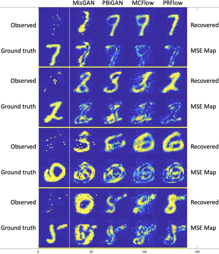
Figure 2: Sample results on MNIST for 80 and 90% missing
rates (top to bottom image groups). behind. PRFlow has the overall edge in image quality
with sharper edges, smoother backgrounds and more real-
istic reconstructions. Specifically, the edges of the plane
image (top row) and ground truth (bottom row) in the left- and mountains against the sky are sharp in PRFlow recon-
most column of each image group. The remaining images structions; the edges of sunglasses against skin are better
in the top row of each group correspond to reconstructions defined; skin textures are more realistic and facial features
by MisGAN, PBiGAN, MCFlow and PRFlow, respectively, (e.g., mouth, nose, hair strands) are rendered more natu-
from left to right. The bottom row in each group includes rally. While there are similarities between the MCFlow and
the mean squared error maps between the reconstruction PRFlow renditions, there are edge sharpness and texture dif-
by each method and the ground truth. Fig. 2 includes re- ferences (e.g., ringing and blockiness artifacts being more
sults across different rates of missing data. It can be ob- pronounced in the MCFlow images) that likely lead to the
served that, as the results from Table 1 indicate, GAN- measurable gap in performance showcased in Tables 1-3.
based methods tend to produce higher MSE reconstructions. Lastly, the bottommost row in Fig. 5 illustrates a subtle but
Further, the reconstructions produced by PRFlow showcase semantically significant reconstruction artifact where com-
human-like handwriting across all levels, with strokes that peting methods hallucinate a person with open eyes, while
are mostly continuous and largely uninterrupted. Lastly, PRFlow accurately reconstructs a squinting face. We invite
the images recovered by PRFlow almost always resemble readers to attempt to fill in missing values themselves from
a readable digit, which is not the case with the competing the partially observed versions of the images. It can be a
methods, particularly for missing rates of 80% and above. challenging task, in particular for high rates of missing data.
Fig. 3 focuses on the 90% missing data case and pro- We should note that humans have an advantage in that they
vides four additional examples. As before, all of the im- know from experience what a number, an animal, or a face
ages restored by PRFlow resemble human-like handwritten look like, whereas the algorithms competing herein were
digits. Failure to recover the original semantic content of never exposed to a single fully observed image, and thus
the images happens mostly in cases where the original im- have to infer what the different objects look like by piecing
ages themselves are ambiguous. Figs. 4 and 5 include re- together fractional observations from multiple images in the
construction results on CIFAR-10 and CelebA. From left to complete absence of labels.
right, the images include: ground truth, observed, and re-
constructions by MNIST, PBiGAN, MCFlow and PRFlow. 5. Discussion
It can be seen that the Flow-based methods outperform the Traditionally, learning from incomplete or partially ob-
GAN-based methods, with PBiGAN lagging significantly served data has meant that trade-offs between various im-Figure 4: Sample results on CIFAR-10. From left to right: ground truth, observed, and MisGAN, PBiGAN, MCFlow and PRFlow reconstructions. Figure 5: Sample results on CelebA. From left to right: ground truth, observed, and MisGAN, PBiGAN, MCFlow and PRFlow reconstructions. age quality aspects had to be incurred. Specifically, prior trend was due to the increasing level of ill-posedness of the methods on image imputation suffered at one or more of recovery process and proposed a regularization approach the following image quality attributes: (i) realism, (ii) pixel- that proved effective at addressing the three-pronged image level quality, and (iii) semantic consistency between the re- quality trade-off. Extensive experimental results demon- covered and the partially observed image. These trade-offs strate that the proposed algorithm consistently matches or became more significant as the degree of data paucity grew outperforms the performance of competing state-of-the-art and approached unity. We hypothesize that this undesirable approaches across all quality metrics in question. The seam-
less incorporation of domain knowledge in the form of a                [13] Ian Goodfellow, Jean Pouget-Abadie, Mehdi Mirza, Bing
prior regularizer was made possible by the formulation of                   Xu, David Warde-Farley, Sherjil Ozair, Aaron Courville, and
the learning task as a joint optimization objective.                        Yoshua Bengio. Generative adversarial nets. In Z. Ghahra-
                                                                            mani, M. Welling, C. Cortes, N. D. Lawrence, and K. Q.
References                                                                  Weinberger, editors, Advances in Neural Information Pro-
                                                                            cessing Systems 27, pages 2672–2680. Curran Associates,
 [1] Panos Achlioptas, Olga Diamanti, Ioannis Mitliagkas, and               Inc., 2014. 1, 2
     Leonidas Guibas. Learning representations and genera-             [14] Ian J. Goodfellow. NIPS 2016 tutorial: Generative adversar-
     tive models for 3D point clouds. In Jennifer Dy and An-                ial networks. CoRR, abs/1701.00160, 2017. 1, 2
     dreas Krause, editors, Proceedings of the 35th International      [15] Kaiming He, X. Zhang, Shaoqing Ren, and Jian Sun. Deep
     Conference on Machine Learning, volume 80 of Proceed-                  residual learning for image recognition. 2016 IEEE Confer-
     ings of Machine Learning Research, pages 40–49, Stock-                 ence on Computer Vision and Pattern Recognition (CVPR),
     holmsmässan, Stockholm Sweden, 10–15 Jul 2018. PMLR.                  pages 770–778, 2016. 6
     1
                                                                       [16] Martin Heusel, Hubert Ramsauer, Thomas Unterthiner,
 [2] Andrew Brock, Jeff Donahue, and Karen Simonyan. Large
                                                                            Bernhard Nessler, and Sepp Hochreiter. GANs trained by a
     scale GAN training for high fidelity natural image synthe-
                                                                            two time-scale update rule converge to a local nash equilib-
     sis. In International Conference on Learning Representa-
                                                                            rium. In Advances in neural information processing systems,
     tions, 2019. 1
                                                                            pages 6626–6637, 2017. 5
 [3] Nadav Cohen and Amnon Shashua. Inductive bias of deep
                                                                       [17] Zhiting Hu, Xuezhe Ma, Zhengzhong Liu, Eduard Hovy, and
     convolutional networks through pooling geometry. In 5th In-
                                                                            Eric Xing. Harnessing deep neural networks with logic rules.
     ternational Conference on Learning Representations, ICLR
                                                                            In Proceedings of the 54th Annual Meeting of the Associa-
     2017, Toulon, France, April 24-26, 2017, Conference Track
                                                                            tion for Computational Linguistics (Volume 1: Long Papers),
     Proceedings. OpenReview.net, 2017. 3
                                                                            pages 2410–2420, Berlin, Germany, Aug. 2016. Association
 [4] A. K. Dey and F. H. Ruymgaart. Direct density estimation
                                                                            for Computational Linguistics. 2
     as an ill-posed inverse estimation problem. Statistica Neer-
     landica, 53(3):309–326, 1999. 2                                   [18] Zhiting Hu, Zichao Yang, Russ R Salakhutdinov, Lianhui
                                                                            Qin, Xiaodan Liang, Haoye Dong, and Eric P Xing. Deep
 [5] Laurent Dinh, David Krueger, and Yoshua Bengio. Nice:
                                                                            generative models with learnable knowledge constraints. In
     Non-linear independent components estimation. CoRR,
                                                                            S. Bengio, H. Wallach, H. Larochelle, K. Grauman, N. Cesa-
     abs/1410.8516, 2014. 2, 3
                                                                            Bianchi, and R. Garnett, editors, Advances in Neural Infor-
 [6] Laurent Dinh, Jascha Sohl-Dickstein, and Samy Bengio.
                                                                            mation Processing Systems 31, pages 10501–10512. Curran
     Density estimation using real NVP.           In 5th Interna-
                                                                            Associates, Inc., 2018. 2
     tional Conference on Learning Representations, ICLR 2017,
     Toulon, France, April 24-26, 2017, Conference Track Pro-          [19] Sergey Ioffe and Christian Szegedy. Batch normalization:
     ceedings. OpenReview.net, 2017. 1, 2, 3, 4, 6                          Accelerating deep network training by reducing internal co-
                                                                            variate shift. volume 37 of Proceedings of Machine Learn-
 [7] Jeff Donahue, Philipp Krähenbühl, and Trevor Darrell. Ad-
                                                                            ing Research, pages 448–456, Lille, France, 07–09 Jul 2015.
     versarial feature learning. In 5th International Conference
                                                                            PMLR. 2
     on Learning Representations, ICLR 2017, Toulon, France,
     April 24-26, 2017, Conference Track Proceedings. OpenRe-          [20] Jian Sun, Zongben Xu, and Heung-Yeung Shum. Image
     view.net, 2017. 2                                                      super-resolution using gradient profile prior. In 2008 IEEE
 [8] Vincent Dumoulin, Mohamed Ishmael Diwan Belghazi, Ben                  Conference on Computer Vision and Pattern Recognition,
     Poole, Alex Lamb, Martin Arjovsky, Olivier Mastropietro,               pages 1–8, 2008. 2
     and Aaron Courville. Adversarially learned inference. 2017.       [21] Durk P Kingma and Prafulla Dhariwal. Glow: Generative
     2                                                                      flow with invertible 1x1 convolutions. In S. Bengio, H. Wal-
 [9] H.W. Engl, M. Hanke, and A. Neubauer. Regularization                   lach, H. Larochelle, K. Grauman, N. Cesa-Bianchi, and R.
     of Inverse Problems. Mathematics and Its Applications.                 Garnett, editors, Advances in Neural Information Processing
     Springer Netherlands, 1996. 2                                          Systems 31, pages 10215–10224. Curran Associates, Inc.,
[10] T. Evgeniou, M. Pontil, and T. Poggio. Regularization net-             2018. 1, 2, 3
     works and support vector machines. Advances in Computa-           [22] Diederik P Kingma and Max Welling. Auto-encoding varia-
     tional Mathematics, 13(1), 2000. 2                                     tional bayes, 2013. cite arxiv:1312.6114. 1, 2
[11] Kuzman Ganchev, João Graça, Jennifer Gillenwater, and Ben       [23] B. Kiran, Dilip Thomas, and Ranjith Parakkal. An overview
     Taskar. Posterior regularization for structured latent variable        of deep learning based methods for unsupervised and semi-
     models. J. Mach. Learn. Res., 11:2001–2049, Aug. 2010. 2               supervised anomaly detection in videos. Journal of Imaging,
[12] Dileep George, Wolfgang Lehrach, Ken Kansky, Miguel                    4(2):36, Feb 2018. 1
     Lázaro-Gredilla, Christopher Laan, Bhaskara Marthi,              [24] Dilip Krishnan and Rob Fergus. Fast image deconvolution
     Xinghua Lou, Zhaoshi Meng, Yi Liu, Huayan Wang, Alex                   using hyper-laplacian priors. In Y. Bengio, D. Schuurmans,
     Lavin, and D. Scott Phoenix. A generative vision model                 J. D. Lafferty, C. K. I. Williams, and A. Culotta, editors, Ad-
     that trains with high data efficiency and breaks text-based            vances in Neural Information Processing Systems 22, pages
     captchas. Science, 358(6368), 2017. 2                                  1033–1041. Curran Associates, Inc., 2009. 2, 3
[25] Alex Krizhevsky, Geoffrey Hinton, et al. Learning multiple and R. Garnett, editors, Advances in Neural Information Pro-
layers of features from tiny images. Technical report, Cite- cessing Systems, volume 32. Curran Associates, Inc., 2019.
seer, 2009. 5 1
[26] Yann Lecun, Léon Bottou, Yoshua Bengio, and Patrick [40] Danilo Jimenez Rezende, Shakir Mohamed, and Daan Wier-
Haffner. Gradient-based learning applied to document recog- stra. Stochastic backpropagation and approximate inference
nition. In Proceedings of the IEEE, pages 2278–2324, 1998. in deep generative models. In Eric P. Xing and Tony Jebara,
6 editors, Proceedings of the 31st International Conference on
[27] Yann LeCun and Corinna Cortes. MNIST handwritten digit Machine Learning, volume 32 of Proceedings of Machine
database. 2010. 5 Learning Research, pages 1278–1286, Bejing, China, 22–24
[28] C. Ledig, L. Theis, F. Huszár, J. Caballero, A. Cunningham, Jun 2014. PMLR. 1
A. Acosta, A. Aitken, A. Tejani, J. Totz, Z. Wang, and W. [41] Trevor W. Richardson, Wencheng Wu, Lei Lin, Beilei Xu,
Shi. Photo-realistic single image super-resolution using a and Edgar A. Bernal. MCFlow: Monte carlo flow models for
generative adversarial network. In 2017 IEEE Conference data imputation. In Proceedings of the IEEE/CVF Confer-
on Computer Vision and Pattern Recognition (CVPR), pages ence on Computer Vision and Pattern Recognition (CVPR),
105–114, 2017. 2 June 2020. 1, 2, 4, 5, 6
[29] Steven Cheng-Xian Li, Bo Jiang, and Benjamin Marlin. Mis- [42] Lorenzo Rosasco, Andrea Caponnetto, Ernesto D. Vito,
GAN: learning from incomplete data with generative adver- Francesca Odone, and Umberto D. Giovannini. Learning,
sarial networks. In International Conference on Learning regularization and ill-posed inverse problems. In L. K. Saul,
Representations, 2019. 1, 2, 5, 6 Y. Weiss, and L. Bottou, editors, Advances in Neural In-
[30] Steven Cheng-Xian Li and Benjamin Marlin. Learning from formation Processing Systems 17, pages 1145–1152. MIT
irregularly-sampled time series: A missing data perspec- Press, 2005. 2
tive. In Proceedings of Machine Learning and Systems 2020, [43] Murray Rosenblatt. Remarks on some nonparametric esti-
pages 5756–5765. 2020. 1, 2, 5, 6 mates of a density function. Ann. Math. Statist., 27(3):832–
[31] Ziwei Liu, Ping Luo, Xiaogang Wang, and Xiaoou Tang. 837, 09 1956. 2
Deep learning face attributes in the wild. In Proceedings of [44] Florian Schroff, Dmitry Kalenichenko, and James Philbin.
International Conference on Computer Vision (ICCV), De- Facenet: A unified embedding for face recognition and clus-
cember 2015. 5 tering. In CVPR, pages 815–823. IEEE Computer Society,
[32] C. Ma, Wenbo Gong, José Miguel Hernández-Lobato, Noam 2015. 6
Koenigstein, Sebastian Nowozin, and C. Zhang. Partial vae [45] Nitish Srivastava, Geoffrey Hinton, Alex Krizhevsky, Ilya
for hybrid recommender system. 2018. 2 Sutskever, and Ruslan Salakhutdinov. Dropout: A simple
[33] Gary Marcus. Deep learning: A critical appraisal. CoRR, way to prevent neural networks from overfitting. J. Mach.
abs/1801.00631, 2018. 2 Learn. Res., 15(1):1929–1958, Jan. 2014. 2
[34] Pierre-Alexandre Mattei and Jes Frellsen. MIWAE: Deep [46] Y. Tai, S. Liu, M. S. Brown, and S. Lin. Super resolution
generative modelling and imputation of incomplete data using edge prior and single image detail synthesis. In 2010
sets. In Kamalika Chaudhuri and Ruslan Salakhutdinov, ed- IEEE Computer Society Conference on Computer Vision and
itors, Proceedings of the 36th International Conference on Pattern Recognition, pages 2400–2407, 2010. 2
Machine Learning, volume 97 of Proceedings of Machine [47] M. Takahashi. Statistical inference in missing data by mcmc
Learning Research, pages 4413–4423, Long Beach, Califor- and non-mcmc multiple imputation algorithms: Assessing
nia, USA, 09–15 Jun 2019. PMLR. 2 the effects of between-imputation iterations. Data Science
[35] Takeru Miyato, Toshiki Kataoka, Masanori Koyama, and Journal, 16(37):1–17, 2017. 3
Yuichi Yoshida. Spectral normalization for generative ad- [48] Niket Tandon, Aparna S. Varde, and Gerard de Melo. Com-
versarial networks. In International Conference on Learning monsense knowledge in machine intelligence. SIGMOD
Representations, 2018. 1 Rec., 46(4):49–52, Feb. 2018. 2
[36] N. Muralidhar, M. R. Islam, M. Marwah, A. Karpatne, and [49] A. N. Tikhonov and V. Y. Arsenin. Solutions of Ill-posed
N. Ramakrishnan. Incorporating prior domain knowledge problems. W.H. Winston, 1977. 2
into deep neural networks. In 2018 IEEE International Con- [50] Dmitry Ulyanov, Andrea Vedaldi, and Victor Lempitsky.
ference on Big Data (Big Data), pages 36–45, 2018. 2 Deep image prior. In Proceedings of the IEEE Conference
[37] Steven J. Nowlan and Geoffrey E. Hinton. Simplifying on Computer Vision and Pattern Recognition (CVPR), June
neural networks by soft weight-sharing. Neural Comput., 2018. 3
4(4):473–493, July 1992. 2 [51] Vladimir N. Vapnik. Statistical Learning Theory. Wiley-
[38] Aaron van den Oord, Sander Dieleman, Heiga Zen, Karen Interscience, 1998. 2
Simonyan, Oriol Vinyals, Alex Graves, Nal Kalchbrenner, [52] Z. Wang, D. Liu, J. Yang, W. Han, and T. Huang. Deep net-
Andrew Senior, and Koray Kavukcuoglu. Wavenet: A gen- works for image super-resolution with sparse prior. In 2015
erative model for raw audio, 2016. cite arxiv:1609.03499. IEEE International Conference on Computer Vision (ICCV),
1 pages 370–378, 2015. 2
[39] Ali Razavi, Aaron van den Oord, and Oriol Vinyals. Gener- [53] Tao Yang, Georgios Arvanitidis, Dongmei Fu, Xiaogang Li,
ating diverse high-fidelity images with vq-vae-2. In H. Wal- and Søren Hauberg. Geodesic clustering in deep generative
lach, H. Larochelle, A. Beygelzimer, F. d'Alché-Buc, E. Fox, models. CoRR, abs/1809.04747, 2018. 1[54] Xitong Yang, Palghat Ramesh, Radha Chitta, Sriganesh
Madhvanath, Edgar A Bernal, and Jiebo Luo. Deep mul-
timodal representation learning from temporal data. In Pro-
ceedings of the IEEE Conference on Computer Vision and
Pattern Recognition, pages 5447–5455, 2017. 1
[55] Jinsung Yoon, James Jordon, and Mihaela van der Schaar.
GAIN: Missing data imputation using generative adversar-
ial nets. In Jennifer Dy and Andreas Krause, editors, Pro-
ceedings of the 35th International Conference on Machine
Learning, volume 80 of Proceedings of Machine Learning
Research, pages 5689–5698, Stockholmsmässan, Stockholm
Sweden, 10–15 Jul 2018. PMLR. 1, 2, 5
[56] Yuxin Zhang, Zuquan Zheng, and Roland Hu. Super reso-
lution using segmentation-prior self-attention generative ad-
versarial network, 2020. 2You can also read