Outlier Detection, Explanation and Prediction: The influence of events on television ratings - MODUL ...
←
→
Page content transcription
If your browser does not render page correctly, please read the page content below
Outlier Detection, Explanation and
Prediction: The influence of events on
television ratings
Bachelor Thesis for Obtaining the Degree
Bachelor of Science
International Management
Submitted to Prof. Lyndon Nixon
Sarah Elisabeth Ilse Fuchs
1511042
Vienna, 31st of May 2019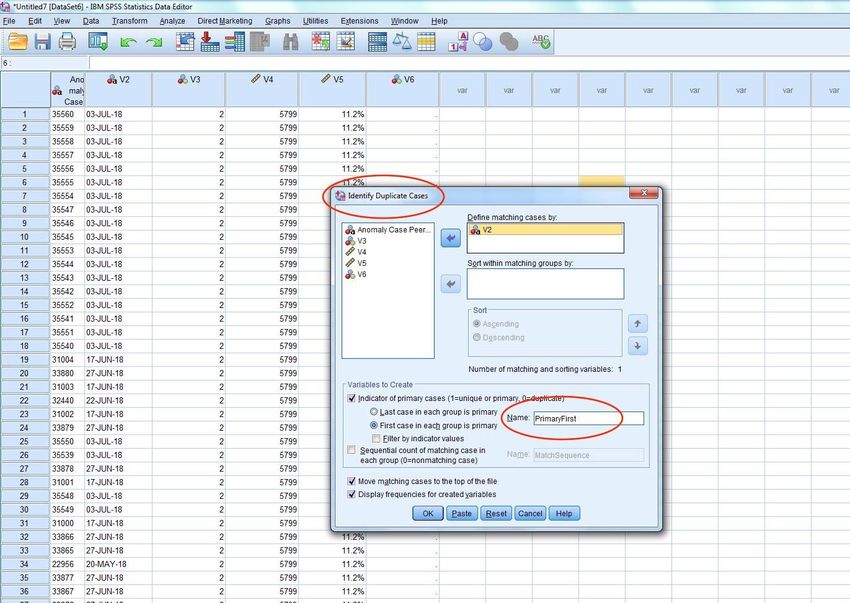
Affidavit
I hereby affirm that this Bachelor’s Thesis represents my own written work and that I have
used no sources and aids other than those indicated. All passages quoted from publications
or paraphrased from these sources are properly cited and attributed.
The thesis was not submitted in the same or in a substantially similar version, not even
partially, to another examination board and was not published elsewhere.
31st of May 2019
Date Signature
2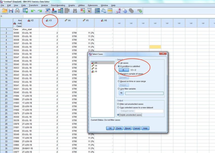
Abstract

This thesis aims to combine the topic of outlier detection together with the prediction of
television ratings. On the basis of TV audience datasets from the OTT streaming platform
Zattoo an outlier detection was performed and the outliers could be matched to certain
events that happened at that date and time. Additionally, it was analysed what the
attributes of TV audience data are and what influence events have on television ratings.
Predicting outliers in data is another topic that has been discussed in this research, in
particular, what influence outliers have on the parameters of forecasting methods. Three
forecasting methods are presented, exponential smoothing, Holt Winters and ARIMA
(p,d,g) and how outliers can be included in the predictions. Along with that, it will be shown
how events can be forecasted through performing a multiple regression. After the
theoretical part follows the analysis of the datasets from OTT streaming platform Zattoo.
Three German channels were investigated, ARD, ZDF and ProSieben. It was seen that
events do have an influence on television ratings by causing particularly large viewing
numbers that were recognized a priori through the outlier detection. Furthermore, it was
found out that the category sports is the dominant category within all the events that were
detected, the other categories being music and politics. The other hypotheses that were
analysed revolve around what influence public holidays have on television ratings, what
happens on another channel while an event is being televised and what influence the
location of the channel has on the events that are streamed. For the last hypothesis two
Swiss channels were chosen, SRF 1 and SRF 2.

                                              3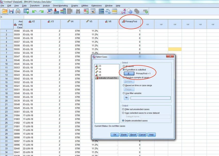
Table of Contents
Affidavit 2
Abstract 3
Table of Contents 4
List of Tables 6
List of Figures 7
1 Introduction 9
2 Outlier Detection, Explanation and Prediction:
The influence of events on television ratings 10
2.1 Outlier Detection and Explanation 10
2.1.1 Definition of Outlier 10
2.1.2 Identification of Outliers: Anomaly detection methods 11
2.1.3 Challenges in Outlier Detection 12
2.1.4 Applications of Outlier Detection 13
2.1.5 The Importance of Explaining Outliers 14
2.2 Predicting Outliers in Time Series 15
2.2.1 Exponential Smoothing Methods 16
2.2.2 Holt–Winters 17
2.2.3 ARIMA Models (Autoregressive Integrated Moving Average) 17
2.3 Predicting Television Ratings 18
2.3.1 The nature of TV audience data 18
2.3.2 Television Prediction Models 19
2.3.3 Why is it important to predict TV audience data? 20
2.4 The role of events in television 20
2.5 Predicting Events and Public Holidays 21
2.6 The Experiment: Combining Anomaly Detection with Prediction of
4
Events in Television 22
2.6.1 Events have an influence on television ratings 23
2.6.2 Sport events influence television ratings more than political events 29
2.6.3 Sport events influence television ratings more than music events 30
2.6.4 The detected anomalies in Swiss television are linked to
different events than in German television 31
2.6.5 With an event being televised on one channel, ratings
on another channel decrease 34
2.6.6 Public holidays have an influence on the number of
television ratings 37
Conclusion 39
Future Work and Limitations 41
Bibliography 42
Appendices 46
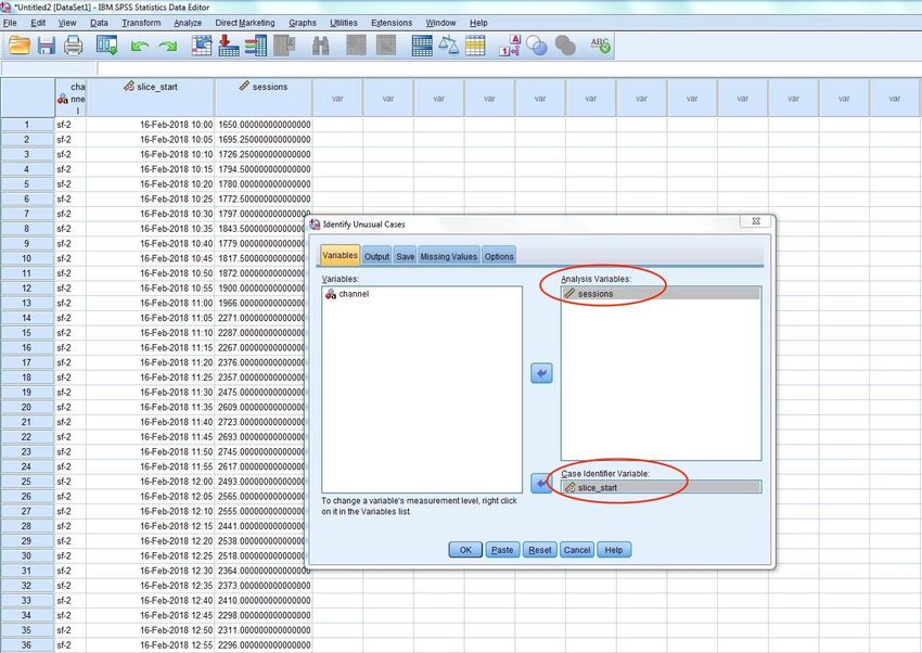
Appendix 1: The Anomaly Detection Process in SPSS 46
Appendix 2: ZDF Event Calendar 49
Appendix 3: ARD Event Calendar 50
Appendix 4: SRF 2 Event Calendar 52
5
List of Tables

Table 1: “True inliers/ outliers versus apparent inliers/outliers” (Retrieved from Zimek and Filzmoser,
2017), p.13

Table 2: Anomaly Case Peer ID List for the Channel ZDF, p.24

Table 3: List of Anomalies After Removal of Duplicates for the Channel ZDF, p.24

Table 4: List of Events That Matched Anomalies for the Channel ZDF, p.25

Table 5: Anomaly Case Peer ID List for the Channel ARD, p.26

Table 6: List of Events That Matched Anomalies for the Channel ARD, p.27

Table 7: List of Anomalies Detected for the Channel ProSieben, p.27

Table 8: List of Events That Matched Anomalies for the Channel ZDF by Categories, p.29

Table 9: List of Events That Matched Anomalies for the Channel ARD by Categories , p.31

Table 10: Anomaly Case Peer ID List for the Channel SRF 1, p.32

Table 11: Anomaly Case Peer ID List for the Channel SRF 2, p.33

Table 12: List of Events That Matched Anomalies for the Channel SRF 2, p.33

Table 13: List of Events That Matched Anomalies for the Channel ZDF with Source Indication, p.49

Table 14: List of Events That Matched Anomalies for the Channel ARD with Source Indication, p.50

Table 15: List of Events That Matched Anomalies for the Channel SRF 2 with Source Indication, p.52

                                                  6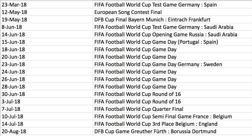
List of Figures
Figure 1: “Most frequent types of outliers”. Retrieved from Upadhyaya and Yeganeh, 2015, p.15

Figure 2: “The electrical equipment orders (top) and its three additive components”. Retrieved from
Hyndman and Athanasopoulos, 2018, p.16

Figure 3: Overview of the Data from the Channels ARD, ZDF and ProSieben, p.23

Figure 4: Result of the Anomaly Detection for the 3rd Peer Group for the Channel ZDF, p.24

Figure 5: Result of the Anomaly Detection for the Channel ZDF After Lowering the Threshold, p.25

Figure 6: Result of the Anomaly Detection for the 3rd Peer Group for the Channel ARD, p.26

Figure 7: Result of the Anomaly Detection for the Channel ARD After Lowering the Threshold, p.26

Figure 8: Result of the Anomaly Detection for the Channel ProSieben, p.27

Figure 9: The Dataset from the 22nd of February 2018 on ProSieben, p.28

Figure 10: The Datasets from ZDF and ARD on the 19th of May 2018, p.30

Figure 11: Overview of the Data from SRF 1, p.31

Figure 12: Result of the Anomaly Detection for the Channel SRF 1, p.32

Figure 13: The Dataset on the 16th of April 2018 on SRF 1, p.32

Figure 14: Overview of the Data from SRF 2, p.33

Figure 15: Result of the Anomaly Detection for the Channel SRF 2, p.33

Figure 16: A Comparison of the Data from the Channels ARD and ZDF from the 14th of June Until the
14th of July 2018, p.34

Figure 17: A Comparison of the Data from the Channels ARD and ZDF from the 19th Until the 25th of
June 2018, p.35

Figure 18: A Comparison of the Data from the Channels ARD and ZDF from the 19th of June 2018, p.
35

                                                   7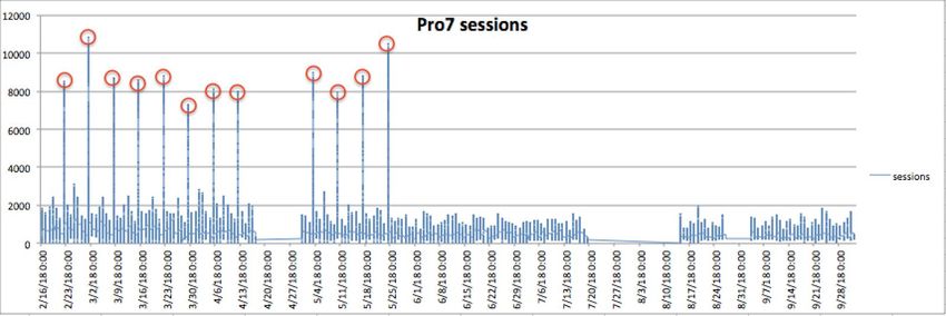
Figure 19: The Expected Curve from the Channel ARD in Comparison With the Data from ZDF from
the 19th of June 2018, p.36

Figure 20: A Comparison of the Data from the Channels ARD and ZDF from the 23rd of June 2018,
p.37

Figure 21: The Dataset from the 1st of May 2018 on ZDF, p.38

Figure 22: The Dataset from the 20st of May 2018 on SRF 2, p.38

Figure 23: The Dataset from the 16th of April 2018 on SRF 1, p.38

Figure 24: An example of “Identify Unusual Cases” in SPSS, p.46

Figure 25: The Imported Table of the Peer Groups in SPSS, p.47

Figure 26: An Example of the Command “Select Cases”, p. 47

Figure 27: An Example of the Command “Identify Duplicate Cases”, p.48

Figure 28: Selecting Duplicate Cases, p.48

Figure 29: The Result of the Anomaly Detection After Removal of Duplicates, p.49

                                                 8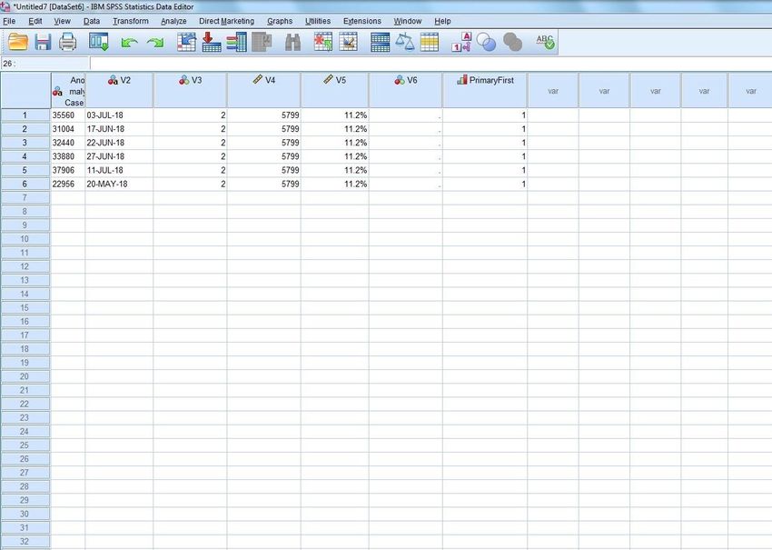
1       Introduction

Outliers are one of the most discussed topics in the field of Statistics. Hardly any dataset or
statistic can be found that does not have any outlying observations. The concept of
normality and abnormality is one that is discussed by scientists in various fields, let it be
biology or anthropology, psychology or statistics. While outliers are often seen as a
disturbance to the data, this thesis aims to show that irregularities can also hold valuable
information when taking a closer look at them after they have been identified through an
anomaly detection. At the same time, this research looks at the question, what influence
events have on TV audience data. With applications like Netflix, Hulu or Amazon Prime
television ratings have dropped tremendously and households have started to refrain from
paying for television as a study from 2018 shows (eMarketer, 2018). However, when it
comes to events that are streamed on television it can be seen that these are still widely
popular to be watched on TV. The TV audience data analysed shows that at certain times
viewing numbers are unusually high, in fact that these are outlying observations in the
data, and the times could be matched to certain events that occurred and that were shown
on television.
Furthermore, predicting outlying observations in time series is also a major issue in
forecasting practices. While it is well known how to deal with seasonality, trend and cyclical
behaviour, there is no method found that can include outliers into prediction methods. This
thesis aims to give an overview over forecasting models that managed to predict anomalies
under certain circumstances.
There are three major research questions that are being answered in this thesis:

    1) What are the different mechanisms to detect anomalies?
    2) Through identifying and explaining outliers, can irregularities be seen as something
        useful rather than a disturbance to the data?
    3) Do events have an influence on television ratings?

The first part of this thesis consists of a literature review which looks at definitions of
outliers and outlier detection mechanisms followed by an overview of forecasting methods,
in particular Exponential Smoothing, Holt Winters, ARIMA and a multiple regression model.
It will be examined what the nature of TV audience data is and what role events play in
television. The second part of the thesis is the practical research, where TV audience data is
being analysed and six hypotheses are tested on TV audience data from the OTT streaming

                                              9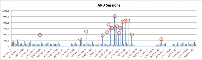
platform Zattoo. This thesis is written in cooperation with the European Union funded
project “ReTV”, an initiative to revise concepts of television in the Internet age.
2 Outlier Detection, Explanation and Prediction: The influence of
events on television ratings
2.1 Outlier Detection and Explanation
2.1.1 Definition of Outlier
There are many different definitions that explain what outliers are. Barnett and Lewis
(1994, p.4) define an outlier as “an observation (or subset of observations) which appears
to be inconsistent with the remainder of that set of data”. Grubbs (1969) stated that “an
outlying observation, or outlier, is one that appears to deviate markedly from other
members of the sample in which it occurs”, as quoted in Barnett and Lewis (1994, p.22).
Aggarwal and Yu (2001) declare that “an outlier is defined as a data point which is very
different from the rest of the data based on some measure” (Aggarwal and Yu, 2001,
p.211). These definitions show that for an outlier to be an outlier depends on the rest of
the sample data and what is defined as normality. Zimek and Filzmoser (2018) give an
interesting thought on the topic of defining outliers by pointing out that most definitions
use terms like “appear” or “some measure” or “under the suspicion”. For decades the
focus on outliers has been to create algorithms in order to detect them most efficiently, but
it is also important to consider what an outlier possibly means. An outlier merely declares
that there is the suspicion of a deviation from the norm or that it appears t o be inconsistent
from the rest of the data. These are assumptions, and even if a detection mechanism has
been used it shows that outlying observations have to be handled very carefully. Kruskal
(1960), as quoted in Zimek and Filzmoser (2018), uttered that:
“An apparently wild (or otherwise anomalous) observation is a signal that says: ‘Here is
something from which we may learn a lesson, perhaps of a kind not anticipated
beforehand, and perhaps more important than the main object of the study.’ “
This idea will be discussed further along in this research. Moreover, in this thesis the term
anomaly or irregularity will be treated as a synonym for outlier, the same counts for
10“novelty detection, anomaly detection, noise detection, deviation detection or exception
mining” (Hodge and Austin, 2004, p.85) for outlier detection.
2.1.2 Identification of Outliers: Anomaly detection methods
In this chapter it will be analysed how outliers can be detected. A variety of techniques
exist and there is no model that can be applied universally (Hodge and Austin, 2004). In this
research, an overview of existing techniques will be given, however, it is impossible to
provide all existing approaches.
Outlier detection approaches can be categorised in different ways (Su and Tsai, 2011).
Hodge and Austin (2004) differ between the three fields, Statistics, Neural Networks and
Machine Learning. In Statistics, there is a differentiation between parametric and
non-parametric approaches, whereas Neural Networks and Machine Learning is divided in
unsupervised, supervised and semi-supervised approaches to outlier detection (Su and
Tsai, 2011). In unsupervised outlier detection, there is no preceding label available for the
data, thus an observation could be normal or anomalous (Su and Tsai, 2011). Hodge and
Austin (2004) call this a Type 1 outlier detection model. Here outliers are detected “with no
prior knowledge of the data” and the most outlying points are marked as potential
anomalies (Hodge and Austin, 2004, p.88).
In supervised outlier detection, pre-labelled data is necessary for training in order to build a
classifier (Hodge and Austin, 2004). The approach usually contains two phases, “a training
phase and a testing phase” (Patcha and Park, 2007, p.3452). In the training phase the
model learns what is normal and what is abnormal data and in the testing phase this profile
can be used on new data. (Patcha and Park, 2007). This is corresponding to “supervised
classification” and forms the Type 2 outlier detection model (Hodge and Austin, 2004).
A semi-supervised approach is a hybrid of Type 1 and Type 2. It can recognize normality
and if a data point lies outside the borders of normality the model declares it as a novelty
(Hodge and Austin, 2004). Here abnormal data does not need to be available precedingly
unlike with a Type 2 model.
However, some of the earliest algorithms for detecting outliers were created in the field of
statistics. An informal way is the Boxplot, which can “identify outliers that have extremely
large or small X values” (Su and Tsai, 2011, p.262). The Boxplot shows the lower extreme,
lower quartile, median, upper quartile and upper extreme (Laurikkala et al, 2000). The
11threshold for an upper or lower outlier is 1.5x of the interquartile range, which is an upper
quartile minus the lower quartile (Laurikkala et al, 2000). Barnett and Lewis (1994) pose the
rule that all data points that are three standard deviations away from the mean should be
marked as outliers. This is also known as the z-score, the number of standard deviations
away from the mean, which was originally created by Grubbs in 1969 (Chandola et al,
2009). The z-score is computed by the formula:
z= |x− x ̅|/ s,
with x ̅ being the mean and s being the standard deviation. The formula for computing
whether a data point is anomalous is:
/(2N) ,N− 2 “is a threshold used to declare an instance to be
N is the size of the test data and tα
anomalous or normal” (Chandola et al, 2009, p. 31). The threshold is important as it
controls the number of data points that are marked as anomalous (Chandola et al, 2009).
Anomaly detection in statistics is divided into parametric and nonparametric models. In
parametric approaches, it is assumed prior to the anomaly detection that “data
distributions are Gaussian in nature” (Markou and Singh, 2003, p.2483) “and certain
parameters are calculated to fit the distribution” (Markou and Singh, 2003, p.2483).
Nonparametric approaches have no predefined model structure, however it is figured out
once the data is given (Chandola et al, 2009). Therefore nonparametric methods “give
greater flexibility” (Markou and Singh, 2003, p. 2483). The most used model is the
histogram based anomaly detection for a univariate dataset. This is especially used in
intrusion detection (ibid.).
2.1.3 Challenges in Outlier Detection
One of the biggest challenges in outlier detection poses the issue when an outlier is close to
the border of normality or a data point lies just within the normal region and is therefore
not considered as an outlier but might actually be one (Singh and Upadhyaya, 2012). In
other words, the borderline between normality and anomaly can be imprecise (ibid.).
Furthermore, it has to be considered that the concept of what is normal can be emerging
12and developing, that the human tastes and preferences are changing over time and what is
normal now “may not be current to be a representative in the future” (ibid.).
Another challenge is the confusion of an anomaly with noise (Chandola et al, 2009). García
et al (2013) state that “in some studies outliers are also regarded as noisy data, although
they are actually extreme or exceptional, but correct, cases” and that “noisy data may harm
the learning process”, whereas outliers are something that can be learnt from (García et al,
2013, p.620).
Moreover, only few anomaly detection methods are applicable universally. Most
approaches are created for a specific problem, especially because the notion of an anomaly
changes in different fields of application (Singh and Upadhyaya, 2012). As Chandola et al
(2009) state:
“In the medical domain a small deviation from normal (e.g., fluctuations in body
temperature) might be an anomaly, while similar deviation in the stock market domain
(e.g., fluctuations in the value of a stock) might be considered as normal”
Another important aspect to consider is the labeling. Table 1 shows the difference between
true and false positives. When a true inlier is marked as an apparent outlier it is a false
positive and vice versa, if a true outlier is marked as an apparent inlier it is a false negative.
Apparent outliers Apparent inliers
True outliers True positives False negatives
True inliers False positives True negatives
Table 1: “True inliers/ outliers versus apparent inliers/outliers” (Retrieved from Zimek and Filzmoser, 2017)
2.1.4 Applications of Outlier Detection
Outlier detection has a wide range of applications, the most common fields are fraud
detection, intrusion detection and fault detection (Chandola et al, 2009). Fraud detection is
often used for credit card fraud and loan application fraud or in the insurance or health
care sector (ibid.). Intrusion detection is used in cyber-security when “detecting
unauthorized access in computer networks” (Hodge and Austin, 2004, p.88). Fault
detection describes when faults are being diagnosed in “safety critical systems” (Chandola
13et al, 2009, p.2). An extensive list of more applications of outlier detection can be found in
the survey of outlier detection methodologies by Hodge and Austin (2004).
2.1.5 The Importance of Explaining Outliers
Outlier explanation or interpretation is an equally important topic as detecting anomalies.
It is important to explain outliers once they are detected as an outlier is an indication of
“abnormal running conditions” (Hodge and Austin, 2004, p.86) and “offers [...] a facility to
gain insights into why an outlier is exceptionally different from other regular objects” (Dang
et al, 2013, p.305).
Outlying observations in data occur for one of the following reasons: “human error,
instrument error, natural deviations in populations, fraudulent behaviour, changes in
behaviour of systems or faults in systems” (Hodge and Austin, 2004, p.87). After its
detection one is put with the question whether the outlier should be removed or retained.
An answer is given by Hodge and Austin (2004): If the outlier is the result of a technical or
human error, the observation should be replaced with a normal value or removed.
However, if the anomaly is because of natural deviations or changes in behaviour it is
crucial that the outlier is retained as it is an indication of anomaly due to external reasons.
If the outlier is a result of fraudulent behaviour or fault in a system an administrator should
be alarmed immediately to deal with the situation. Afterwards the data point may be
corrected although in a separate file so that the original dataset is not affected but the data
can be used for future work, as outliers affect the mean and median of the data.
142.2 Predicting Outliers in Time Series
Time series forecasting is an important part of any business nowadays. Through analyzing
past values the aim is to predict future values. There are many models available that can
recognize seasonality and trend, for example the Holt-Winters or the seasonal ARIMA
model. However, including anomalies into forecasts is a topic that is still not developed
entirely. In the following, an overview of different forecasting methods will be given and
how they can include outliers. But first, it is necessary to look at the different types of
anomalies in temporal data, which are additive outlier (AO), transitory change and level
shift (Upadhyaya and Yeganeh, 2015).
Figure 1: “Most frequent types of outliers”. Retrieved from Upadhyaya and Yeganeh, 2015
In this research, the focus will be on additive outliers. Additive outliers are “single
observations that are surprisingly large or small, independent of the neighbouring
observations” (Talagala et al, 2018, p.5).
Time series in general can be decomposed into the following three components, the trend,
seasonal and remainder component. The remainder component is also called the irregular
component. Figure 2 shows the data set and its three components.
15Figure 2: “The electrical equipment orders (top) and its three additive components”. Retrieved from Hyndman
and Athanasopoulos, 2018
Considering an additive decomposition, the formula is yt=St+Tt+Rt, where “yt is the data, St
is the seasonal component, Tt is the trend-cycle component, and Rt is the remainder
component, all at period t” (Hyndman and Athanasopoulos, 2018, p.157).
2.2.1 Exponential Smoothing Methods
Exponential smoothing is a forecasting method that uses weighted averages, which give
more weight to more recent observations. Simple exponential smoothing does not allow to
use data with seasonality or trend and the time series should be stationary. The smoothing
parameter α with a value between 0 and 1 indicates the weight given to past
observations. If α is 1, all the weight lies on the last observation, hence it would be a Naive
1 method. (Hyndman and Athanasopoulos, 2018). Double exponential smoothing can
include a trend component. This method consists of the smoothing parameter α as
mentioned before and a base term a and trend term b for the trend.
However, in exponential smoothing outliers can affect the parameter estimations and thus
the forecasts tremendously (Koehler, 2012). Methods have been developed that allow to
use exponential smoothing despite the presence of outliers. The majority of methods focus
on replacing the outlier with a normal value or treating an outlier as a missing value
16(Hyndman and Athanasopoulos, 2018). One exemplary procedure is presented by Koehler
et al (2012). Here a so called outlier forecasting procedure is applied, which starts with an
iterative search for all three kinds of potential outliers, namely additive outliers, a level
shift or a transitory change. The search ends when no new outliers can be found. An
innovative state space model is applied which assumes that there are no outliers. The
outlier forecasting procedure can “adjust for outliers” and can be “applied automatically”
(Koehler et al, 2012). Accommodating outliers is especially difficult when they are located
towards the end of the time series. If outliers are present in the beginning of a series,
exponential smoothing can work fairly well as most of the weight is given to the most
recent observations and less weight to older data (Koehler et al, 2012).
2.2.2 Holt–Winters
The Holt- Winters method can accommodate trend and seasonality. The seasonality is
expressed through a seasonal component s and the frequency of the seasonality is
indicated by m (e.g. for monthly data m equals 12). There is an additive and a multiplicative
model. The multiplicative model assumes that the seasonality is changing proportionally to
the level of the time series, whereas the additive model is suggested when the seasonal
changes are more or less consistent throughout the timeline (Hyndman and
Athanasopoulos, 2018).
Again, both methods are unsuitable for time series that contain outliers but some
procedures exist to deal with them. One way is presented by Andrysiak et al (2018), where
the Holt-Winters model is combined with anomaly detection in the context of network
intrusion. Rather than scanning the network traffic data for attacks, it is first defined what
is the normal traffic and then any deviations from the norm are marked as possible attacks
(Andrysiak et al, 2018). When all data lies “within the calculated prediction intervals, we
assume that there is no attack/anomaly in out network” (Andrysiak et al, 2018, p.573). If
the data outreaches the proposed interval, there is an alarm and it is noted to the log. This
method is particularly created for automation.
2.2.3 ARIMA Models (Autoregressive Integrated Moving Average)
ARIMA models are the models that are most applied when it comes to dealing with outliers
in time series forecasts. While exponential smoothing models “are based on a description
of the trend and seasonality in the data”, ARIMA models “aim to describe the
autocorrelations in the data” (Hyndman and Athanasopoulos, 2018, p.221). Just like a
17multiple regression can use several predictors, forecasting here works by using a “linear
combination of past values of the variable” (Hyndman and Athanasopoulos, 2018, p.221).
These past values are also called lagged values. A non-seasonal ARIMA model can be
written as an ARIMA (p,d,g) model, where p is the order of the autoregressive part, d is the
degree of first differencing involved and g is the order of the moving average part
(Hyndman and Athanasopoulos, 2018).
The forecasting method developed by Chen and Liu (1993b) is the most used and cited
when it comes to predicting outliers in time series. The main issues addressed in their
research is the fact that outliers have a tremendous impact on the parameter estimates
which leads to inaccurate forecasts and that the masking effect results in some anomalies
not being detected (Chen and Liu, 1993a). However, when type and location of the outlier
are known, “one can adjust the outlier effects on the observations and the residuals” (Chen
and Liu, 1993a, p.286).
2.3 Predicting Television Ratings
2.3.1 The nature of TV audience data
Predicting television ratings is surprisingly an area that has not been given much attention
to by research, as Danaher et al (2011) state, even though the field is rapidly developing,
from access methods like satellite and cable to the Internet and mobile phone accessibility.
The number of channels is also increasing. This makes the nature of TV audience data quite
complex and on top of all these challenges, the data is highly seasonal (Danaher et al,
2011). Having winter months as peaks and summer months with daylight saving making
numbers drop, to weekly seasonality with more viewers on weekends than on weeknights
up to a daily seasonal pattern with prime time between 8 and 10 pm (Danaher et al, 2011).
Additional to that, there is also variance across days, for example “the largest total
audiences at 6 pm and 8 pm are generally on Sundays and Mondays, while viewing at 10
pm is highest on a Saturday” (Danaher et al, 2011, p.1218). Furthermore, television rates or
television usages are determined by additional components. There is audience availability
and audience demographics on the demand side along with behavioral attributes of the
viewers whereas program content and scheduling is on the supply side (Weber, 2002). Also
other factors like cast demographics can play a role (Meyer and Hyndman, 2006).
Additionally, it is also important to mention how television ratings are created. The most
famous way of generating television ratings is the one by Nielsen in the US. In the 1950s
18Nielsen started to collect data from several households, called the “Nielsen families”. These
families wrote in diaries about their television viewing habits (Roussanov, 2016). Around 25
years later, in 1987, the People Meter was invented by Nielsen, a small box next to the
television that was measuring when and what the household members are watching on
television. Even nowadays this method is still used, with Nielsen taking the data from
around 40,000 households - thus relying on a sample population in order to create overall
viewing numbers (Roussanov, 2016).
2.3.2 Television Prediction Models
Predicting television ratings can be divided into two big categories, linear models and
non-linear models. Linear models focus mainly on weighted averages (Weber, 2002), As the
category indicates, the model is linear as time is the main predictor, thus they require
evenly spaced time series (Weber, 2002). However, linear models exist that can include
seasonality like time of the day and day of the week as well as predictors that indicate the
content of a program like cast demographics and programm dummies (Meyer and
Hyndman, 2006). Bortz (1986) for example created a “programme attractiveness index”
(Weber, 2002).
Non-linear models are subdivided into technical and exploratory methods, where
“technical models do not consider exogenous predictors except for the lags of the variable
they are meant to predict” (Weber, 2002, p.2). These methods are mainly seasonal or
distributional. Seasonal models are basic time series methods that are part of many
software programs nowadays. They derive the forecasting information “exclusively from
the seasonality of past TV usage” (Weber, 2002, p.2). Non-linear exploratory models consist
of several predictors of TV usage. This area is fairly recent to data scientists as artificial
intelligence is used and models consider not only seasonality and the program content of
the forecasted channel but also the content of competing channels and the program
surroundings (Weber, 2002).
Along with the traditional forecasting techniques, a Nielsen study shows how analysing
social media can improve forecasts when it comes to predicting television ratings. A
correlation was found between tweets and television ratings and that for example “for
18-34 year olds, an 8.5% increase in Twitter volume corresponds to a 1% increase in TV
ratings for premiere episodes” (Nielsen, 2013). Using the likes, shares and comments on TV
show articles on Facebook or tweets and retweets on Twitter viewers can express their
opinions towards a show or episode. This is valuable information for forecasters as it
19represents the popularity of a series. The Nielsen study considered not only the social
media buzz volume but also television factors like genre and how long the show has been
televised, money spent on advertising the show and past ratings (Subramanyam, 2011).
This shows how important it is to include several predictors into forecasts, with social
media buzz being an innovative part when regarding the digital age of television.
2.3.3 Why is it important to predict TV audience data?
Having considered how to forecast television ratings, it is important to explain why it is
important to do so. The most important reason for predicting viewing numbers is because
advertising prices for television are determined based on the forecasts of audience
numbers (Danaher et al, 2011). If audience numbers have not been attained as projected,
media planners are refunded in an appropriate manner (Meyer and Hyndman, 2006).
Nevertheless the refund does not account for the fact that their media plan has been
disturbed (Meyer and Hyndman, 2006). Therefore it is important to generate as accurate
forecasts as possible.
2.4 The role of events in television
Rather than the weekly occuring national sport events, major events like the Super Bowl,
the Olympic Games or the Football World Cup are the ones that are having the largest
audience numbers since approximately the 1970s (Whannel, 2009). Even though we live in
an age of movie streaming applications like Netflix and Amazon Prime, these mega events
on television are still of major importance. Live television is not only about the sport that is
being seen, but also the feeling of togetherness and unitedness, sharing an experience in
the intimate space of one's home (Whannel, 2009). The Super Bowl in that sense can be
almost seen as a national holiday in the US. But not only in the sociological matter, but also
in economic terms events play a big role in television. Events in television are especially
interesting for advertisers and sponsors. Because of the huge audience numbers even a 30
second advertisement can reach millions of viewers. The most famous example is the Super
Bowl in the US, with 93.1 million television viewers in 2019 (Nielsen, 2019) and
advertisement costs that exceed 5 million dollars per 30 second advertisement (Statista,
2019). This form of revenue stream is essential for television channels.
Another question to consider is how other channels react to a media event being televised.
Do they continue to show their regular television show or do they offer an alternative
program? How do they manage to keep up television ratings? In case of the Super Bowl,
20some answers to these questions could be found. In 1992 Fox started to televise a show
called “In Living Color” which airs directly opposite to the halftime show of the Super Bowl
and ends when the football game is resumed on CBS (Meslow, 2017). Another reaction to
encounter the popularity of the Super Bowl is the “Puppy Bowl” which is shown on the
channel Animal Planet and where puppies play against each other rather than humans. It
has become very popular as an alternative program to the football game. Other channels
have also become successful at counter-programming, for example the channel Comedy
Central is offering a marathon of the series “South Park” and the channel Showtime a “Twin
Peaks” marathon (Meslow, 2017). Similar scenarios occurred during the FIFA Football
World Cup in 2018. Rather than resigning to the football world cup, the German television
channels decided to offer an alternative program. For example during the final of the FIFA
world cup 2014 in Brazil, RTL was showing the movie “Kill the Boss”, Sixx televised the
movie “Election”, RTL 2 the movie “Andromeda” and Arte the film “Loulou” with Gérard
Depardieu (Neumann, 2014). It can be seen that the channels attempted to give an
attractive alternative program to their viewers by televising well-known movies. However,
34.65 million viewers were watching the final game on ARD, which is making up 86.3
percent as the market share, hence 13.7 percent were watching a different channel that
evening (Spiegel Online, 2014).
2.5 Predicting Events and Public Holidays
One successful method presented by Hyndman and Athanasopoulos (2018) for predicting
events and public holidays in time series is using a multiple regression. For example, when
tourist arrivals are forecasted for South Africa in 2010, one should consider the impact of
the Football World Cup in that year. This can be done using dummy variables. The dummy
variable will indicate through 1 = “yes” and 0 = “no” whether a special event has occurred
that day or not. The same accounts for public holidays. This method can also be used when
outliers occur in the data, with the dummy variable removing the effect of the outlier
rather than having to replace the outlier (Hyndman and Athanasopoulos, 2018).
Regression models can be linear or multiple. A linear regression only considers one
predictor, whereas a multiple regression takes several predictors into account. The forecast
variable y is the explained variable, while the predictor variable is the explanatory variable.
A linear regression can be expressed through the formula yt=β0+β1xt+εt where β0
indicates the intercept, β1 the slope, x is the predictor and ε the error term (Hyndman
and Athanasopoulos, 2018).
212.6 The Experiment: Combining Anomaly Detection with Prediction of
Events in Television
The TV audience dataset used for the experiment is derived from the project “ReTV”, which
is funded by the European Union. The project was initiated in January 2018 with the goal to
“re-invent TV for the interactive age” (ReTV, n.d.). There is a separate dataset for each
channel and each dataset contains two variables, “time” and “number of sessions”. The
time variable is evenly spaced as the data has been collected every five minutes. All
datasets start on February the 16th and end on October the 2nd 2018. The data is from
several TV channels from Germany and Switzerland. For the experiment three German
channels have been chosen due to their popularity and representativity, namely ARD, ZDF
and ProSieben, and two Swiss channels have been analysed for the fourth hypothesis, SRF 1
and SRF 2. There is a period of missing values between April 17-30 and July 19 until August
14 on every channel. However, this does not affect the results of the experiment. Below is a
summary of the data from each channel. Due to data protection and privacy reasons the
full TV audience dataset will not be published in this thesis. Furthermore, the dataset will
be considered as a representative sample for the television viewing behaviour of the
respective home country of the channel.
22Figure 3: Overview of the Data from the Channels ARD, ZDF and ProSieben
Six hypotheses were created and tested. The method and results for each hypothesis will
be reported individually.
H1: Events have an influence on television ratings
H2: Sport events influence television ratings more than political events
H3: Sport events influence television ratings more than music events
H4: The detected anomalies in Swiss television are linked to different events than in German
television
H5: With an event being televised on one channel, ratings on another channel decrease
H6: Public holidays have an influence on the number of television ratings
2.6.1 Events have an influence on television ratings
In order to test this hypothesis an anomaly detection has been conducted with the
program SPSS Statistics by IBM. With the command “DETECTANOMALY” or “identify
unusual cases” from the menu bar under DATA the algorithm searches for cases that
deviate “from the norms of their cluster groups” (IBM, n.d.).
The anomaly detection performed through SPSS can additionally report the anomalies
based on peer groups. For example, the channel ZDF has 3 peer groups, with 6.5% forming
the third peer group, 56.6% the second and 36.9% the first adding up to 100% in total.
Below is the result of the anomaly detection case peer ID list for ZDF.
23Table 2: Anomaly Case Peer ID List for the Channel ZDF
After the anomaly detection has been performed, it was necessary to remove the
duplicates, as the goal is to find the date with abnormal numbers of sessions and not the
session per se. The anomaly detection for the third peer group looks as following:
Table 3: List of Anomalies After Removal of Duplicates for the Channel ZDF
The process for removing the duplicates was: SELECT CASES under the condition that the
peer group = 3, so that only the third peer group is shown. With the command IDENTIFY
DUPLICATE CASES and the first case in each group being primary, duplicates are being
removed. Then SELECT CASES again with the condition that only the first primary case is
shown will give back the dates. The full anomaly detection and duplicate removal process is
explained in Appendix 1.
Figure 4: Result of the Anomaly Detection for the 3rd Peer Group for the Channel ZDF
24The four dates indicated are the largest unusual cases detected by SPSS for the channel
ZDF. Together they make up 6.5% of the data. However, when lowering the threshold and
considering the second peer group as well, there are 25 outliers in total.
Figure 5: Result of the Anomaly Detection for the Channel ZDF After Lowering the Threshold
Manually the dates have been associated with events that match the streaming time. The
results as shown below demonstrate that most outliers were associated to a specific event
on that day. The table with the source indication can be found in Appendix 2.
Table 4: List of Events That Matched Anomalies for the Channel ZDF
For the channel ARD the anomaly detection by SPSS gave two peer groups with one
anomaly making up the second one.
25Table 5: Anomaly Case Peer ID List for the Channel ARD
Figure 6: Result of the Anomaly Detection for the 3rd Peer Group for the Channel ARD
After lowering the threshold another time to the second peer group, 18 anomalies have
been detected.
Figure 7: Result of the Anomaly Detection for the Channel ARD After Lowering the Threshold
Again, the anomalies have been matched manually with certain events that fit the exact
streaming time on ARD. The table with the source indication is to be found in Appendix 3.
26Table 6: List of Events That Matched Anomalies for the Channel ARD
For the channel ProSieben the results are the following:
Table 7: List of Anomalies Detected for the Channel ProSieben
Twelve anomalies have been detected by SPSS in the second peer group, making up 27.5%
of the data. In this case, there was no need to lower the threshold as all expected outliers
were detected sufficiently.
Figure 8: Result of the Anomaly Detection for the Channel ProSieben
27All twelve dates could be associated to the TV show “Germany’s Next Topmodel”, as the TV
ratings increased rapidly during the time when the show has been streamed on ProSieben.
The show was running from the 8th of February 2018 until the 24th of May 2018 once a
week every Thursday between 8.15 pm until approximately 10.30 pm (ProSieben, n.d.).
“Germany’s Next Topmodel” is a German casting show that was airing every year since
2006. In 2018 the average viewing number of the season was 2.38 million viewers (Statista,
2018).
The graph below shows one example on the 22nd of February 2018 from 0.00 am to 11.55
pm.
Figure 9: The Dataset from the 22nd of February 2018 on ProSieben
It is unclear whether the twelve dates should be considered as anomalous observations or
rather a temporal pattern or a trend. The TV show “Germany’s Next Topmodel” is not
considered as an event per se. It is assumed that the anomaly detection recognized the
dates as outliers because of the extremely large viewer numbers but in fact it is a recurring
weekly pattern that is occuring due to the TV scheduling at that time.
Furthermore, it is interesting to see the small drops in the dataset above. It is assumed that
these exist because of the advertisement breaks, where people decide to switch to another
channel for a while in order to avoid the commercials. However, this could not be verified
in the data, therefore it remains purely an assumption.
To conclude the first hypothesis, the results from the channels ARD and ZDF show that
events do have a strong influence on television ratings. Each detected anomaly was
associated to an event that occurred at that date and time. However, on the channel
ProSieben the outliers were not associated to an event but to a TV show that was recurring
weekly.
282.6.2 Sport events influence television ratings more than political events
In order to test this hypothesis the results from H1 will be used. For the channel ZDF 25
outliers were detected. Out of those 24 were associated with a sport event and one was
associated to a political event, namely the royal wedding of Prince Harry and Meghan
Markle on the 19th of May 2018. Out of the 24 sport events, one was categorized “other
than football”, which was the ice hockey final between Germany and Russia on the 25th of
February 2018.
20-Feb-18 UEFA Champions League Game Bayern Munich : Beşiktaş
25-Feb-18 Ice Hockey Final Germany : Russia
6-Mar-18 UEFA Champions League Game Paris Saint Germain : Real Madrid
14-Mar-18 UEFA Champions League Game Beşiktaş : Bayern Munich
27-Mar-18 FIFA Football World Cup Test Game Germany : Brazil
3-Apr-18 UEFA Champions League Quarter Final Sevilla : Bayern Munich
11-Apr-18 UEFA Champions League Quarter Final Bayern Munich : Sevilla
1-May-18 UEFA Champions League Semi Final Bayern Munich : Real Madrid
19-May-18 The Royal Wedding Live
26-May-18 UEFA Champions League Final
2-Jun-18 FIFA Football World Cup Test Game Germany : Austria
16-Jun-18 FIFA Football World Cup Second Game Day
17-Jun-18 FIFA Football World Cup Game Germany : Mexico
19-Jun-18 FIFA Football World Cup Game Russia : Egypt
21-Jun-18 FIFA Football World Cup Game Day
22-Jun-18 FIFA Football World Cup Game Day
25-Jun-18 FIFA Football World Cup Game Iran : Portugal
27-Jun-18 FIFA Football World Cup Game Germany : South Korea
FIFA Football World Cup Round of 16; Spain : Russia / Croatia :
1-Jul-18 Denmark
2-Jul-18 FIFA Football World Cup Round of 16; Brazil : Mexico / Belgium : Japan
6-Jul-18 FIFA Football World Cup Quarter Finals
11-Jul-18 FIFA Football World Cup Semi Finals
15-Jul-18 FIFA Football World Cup Finals
24-Aug-18 German Premier League Opening Bayern Munich : Hoffenheim
6-Sep-18 Nations League Football Game Germany : France
Category: Sport event (Football)
Category: Sport event (other than football)
Category: Political
Table 8: List of Events That Matched Anomalies for the Channel ZDF by Categories
29Taking a closer look at one specific example from the 19th of May 2018. ZDF showed from
11 am onwards the Royal Wedding of Prince Harry and Meghan Markle. ARD started
streaming from 8.15 pm the DFB Cup Final. Below are the ratings from both channels on
that day. While ZDF had a peak with around 20 000 viewers, ARD reached more than 50
000 with the sports game.
Figure 10: The Datasets from ZDF and ARD on the 19th of May 2018
It can be seen that the sport event reached a higher quota than the political event in one
specific case, but also in the overall number of detected outliers that were associated to
events as one out of 25 was linked to a political event and 24 to a sport event.
2.6.3 Sport events influence television ratings more than music events
On the channel ZDF 18 outliers were detected. Out of those 17 werde associated with a
sport event and one was in the category of music events, the Eurovision Song Contest on
the 12th of May 2018.
23-Mar-18 FIFA Football World Cup Test Game Germany : Spain
12-May-18 European Song Contest Final
19-May-18 DFB Cup Final Bayern Munich : Eintracht Frankfurt
FIFA Football World Cup Test Game Germany : Saudi
8-Jun-18 Arabia
30FIFA Football World Cup Opening Game Russia : Saudi
14-Jun-18 Arabia
15-Jun-18 FIFA Football World Cup Game Day (Portugal : Spain)
18-Jun-18 FIFA Football World Cup Game Day
20-Jun-18 FIFA Football World Cup Game Day
23-Jun-18 FIFA Football World Cup Game Day Germany : Sweden
24-Jun-18 FIFA Football World Cup Game Day
26-Jun-18 FIFA Football World Cup Game Day
28-Jun-18 FIFA Football World Cup Game Day
30-Jun-18 FIFA Football World Cup Round of 16
3-Jul-18 FIFA Football World Cup Round of 16
7-Jul-18 FIFA Football World Cup Quarter Final
FIFA Football World Cup Semi Final Game France :
10-Jul-18 Belgium
14-Jul-18 FIFA Football World Cup 3rd Place Belgium : England
20-Aug-18 DFB Cup Game Greuther Fürth : Borussia Dortmund
Category: Sport event (Football)
Category: Music
Table 9: List of Events That Matched Anomalies for the Channel ARD by Categories
It can be seen that in the data that has been worked with the category sport event
(football) is dominant. Therefore it has been shown that sport events have a greater
influence on television ratings in the sample data than music events.
2.6.4 The detected anomalies in Swiss television are linked to different events
than in German television
Additional to the German channels two Swiss channels have been analysed, SRF 1 and SRF
2. Both datasets are in the same time frame as the German channels and the data is
retrieved from the same source, ReTV and the application Zattoo. The data for SRF 1 looks
as following:
Figure 11: Overview of the Data from SRF 1
31An anomaly detection has been performed with SPSS. For SRF 1 there are three peer
groups, with one big anomaly making up the first peer group with a peer sice of 25%.
Table 10: Anomaly Case Peer ID List for the Channel SRF 1
Figure 12: Result of the Anomaly Detection for the Channel SRF 1
The outlier was linked to the 16th of April 2018 and associated to a public holiday in
Switzerland, the Spring Celebration in Zurich, also called “Sechseläuten”.
Taking a closer look at the data from that day, the ratings start to increase around 3 pm
with 1232 viewers and the peak was at 4.20 pm with 5245 viewer ratings. SRF1 was live
streaming the festive parade in Zurich for three hours starting at 3.35 pm, which explains
the increase in ratings during that time(SRF, n.d.).
Figure 13: The Dataset on the 16th of April 2018 on SRF 1
For SRF 2, the data looks as following:
32Figure 14: Overview of the Data from SRF 2
The result of the anomaly detection with SPSS gave two peer groups, the second one is
made up of six anomalies accounting for 11.2 % of the data.
Table 11: Anomaly Case Peer ID List for the Channel SRF 2
Figure 15: Result of the Anomaly Detection for the Channel SRF 2
Manually the dates were associated to events that match what has been shown on SRF2
during the outlying time slot. The table with the source indication is to be found in
Appendix 4.
20-May-18 Ice Hockey World Cup Final Sweden : Switzerland
17-Jun-18 FIFA Football World Cup Game Switzerland : Brazil
22-Jun-18 FIFA Football World Cup Game Switzerland : Serbia
27-Jun-18 FIFA Football World Cup Game Switzerland : Costa Rica
03-Jul-18 FIFA Football World Cup Round of 16 Switzerland : Sweden
11-Jul-18 FIFAFootball World Cup Semi Final Croatia : England
Table 12: List of Events That Matched Anomalies for the Channel SRF 2
33The associated events are all sport events that Switzerland was part of except for the last
one, the Semi Final of the FIFA Football World Cup. From this example it can be seen that
the location of the channel has an influence on the events that cause the viewing numbers
to reach an anomalous level as most anomalies were associated to events that Switzerland
was a part in.
2.6.5 With an event being televised on one channel, ratings on another channel
decrease
The goal of the fifth hypothesis is to find out whether an event on one channel influences
the viewer ratings of another channel. The month from the 14th of June until the 14th of
July 2018 has been chosen to compare the two channels ARD and ZDF with each other. As a
result, it could be seen that during that month the spikes of viewing numbers take turn,
meaning that if there is a peak of ratings on ARD, the channel ZDF has a low number of
sessions and vice versa.
Figure 16: A Comparison of the Data from the Channels ARD and ZDF from the 14th of June Until the 14th of
July 2018
Taking a closer look, the graphs below show the week from the 19th of June until the 25th
of June 2018.
34Figure 17: A Comparison of the Data from the Channels ARD and ZDF from the 19th Until the 25th of June 2018
It shows more clearly that every time an event is shown on one channel, the ratings on the
other channel stay low. Furthermore, the goal was also to see whether if viewers watch
one channel, they decide to switch to the other channel or whether they would continue to
watch the regular program that they have been watching at that time. However, in the
dataset no such evidence was found where viewers decide to switch the channel. The data
rather shows tendencies that viewers specifically start to stream the event that they want
to see instead of switching the channel from a previous watched TV show or event. A few
examples will be shown below.
First, an example of the 19th of June 2018 can be seen below. ZDF was streaming the FIFA
Football World Cup Game Russia vs. Egypt.
Figure 18: A Comparison of the Data from the Channels ARD and ZDF from the 19th of June 2018
35The ratings on ARD stay relatively the same until a rapid increase at 6.15 pm to over 5 000
viewers, followed by a decrease and another increase again until the numbers drop
towards midnight. No significant drop on the channel ARD was witnessed, there was even a
sharp increase. However, it is important to consider the significant difference in the
number of ratings, as ZDF experiences almost 60 000 ratings while the peak of viewing
numbers on ARD is at 5 000.
Below the expected curve of ARD is shown. The data from ARD is fictional as this is what
was expected if viewers decide to change the channel.
Figure 19: The Expected Curve from the Channel ARD in Comparison With the Data from ZDF from the 19th of
June 2018
This is the expected scenario. Television viewers that are watching ARD are changing the
channel to see the event streamed on ZDF. ZDF ratings increase, while ARD ratings are
declining at the same time.
In the next example as seen on the next page from the 23rd of June 2018, ARD was
streaming the FIFA Football World Cup Game Germany vs. Sweden. The sessions that day
on ARD had a peak at around 7.45 pm with 103 179 sessions. On ZDF the number of
sessions revolves in a range between 172 and 3608 sessions on the same day. In this case
again no significant change was experienced on ZDF, even though the viewing numbers on
ARD were peaking.
36Figure 20: A Comparison of the Data from the Channels ARD and ZDF from the 23rd of June 2018
To conclude this hypothesis, it could be seen that if one channel televised an event, the
ratings on another channel are low. However, there was no evidence found that viewers
decide to switch from another channel to the event. This indicates a tendency that viewers
decide to specifically turn on the television to watch an event.
2.6.6 Public holidays have an influence on the number of television ratings
It was expected that public holidays have an influence on television ratings as people are
off work and could spend more time watching television that day. In the data that has been
analysed three public holidays come up as anomalies, the 1st of May as the Workers’
Holiday, the 16th of April as the Swiss holiday “Sechseläuten” and the 20th of May as the
Whitsunday.
Figure 21: The Dataset from the 1st of May 2018 on ZDF
On the 1st of May 2018 the channel ZDF streamed the UEFA Champions League semi-final
Bayern Munich vs. Real Madrid. The first of May is also a public holiday called the workers’
day which fell on a tuesday that year. It can be seen that the ratings were low during the
37day. In the evening when ZDF was streaming the football game the numbers were
increasing rapidly and had a peak at 20.15 with 59 249 viewers on Zattoo.
Figure 22: The Dataset from the 20st of May 2018 on SRF 2
On the 20th of May 2018 SRF 2 was streaming from 7.30 pm onwards the final of the Ice
Hockey World Cup between Sweden and Switzerland. Television ratings were low during
the day and rose sharply towards the evening, yet in a slower manner than on ZDF.
Figure 23: The Dataset from the 16th of April 2018 on SRF 1
The 16th of April is a public holiday in Switzerland called “Sechseläuten”. SRF 1 was
streaming the festive parade in Zurich starting at 3.35 pm that which is also the same time
as the ratings were peaking on SRF 1.
To conclude this hypothesis, it can not be clearly said whether the increase in television
ratings on these three dates was a result of the days being public holidays and viewers
having more time to watch television or out of the interest of the viewers in the events that
were being streamed. However, as the ratings are low during the day but only increase
when the event is being streamed it can be said that for the analysed data the fact that the
day was a public holiday was not the reason why television ratings were increasing but
rather the content that was being shown.
38You can also read


