Sentiment-Guided Adversarial Learning for Stock Price Prediction
←
→
Page content transcription
If your browser does not render page correctly, please read the page content below
ORIGINAL RESEARCH
                                                                                                                                                    published: 26 May 2021
                                                                                                                                            doi: 10.3389/fams.2021.601105

                                           Sentiment-Guided Adversarial
                                           Learning for Stock Price Prediction
                                           Yiwei Zhang 1, Jinyang Li 1, Haoran Wang 1 and Sou-Cheng T. Choi 2,3*
                                           1
                                               Beijing Institute of Technology, Haidian District, Beijing, China, 2Kamakura Corporation, Honolulu, HI, United States,
                                           3
                                               Department of Applied Mathematics, Illinois Institute of Technology, Chicago, IL, United States

                                           Prediction of stock prices or trends have attracted financial researchers’ attention for many
                                           years. Recently, machine learning models such as neural networks have significantly
                                           contributed to this research problem. These methods often enable researchers to take
                                           stock-related factors such as sentiment information into consideration, improving
                                           prediction accuracies. At present, Long Short-Term Memory (LSTM) networks is one
                                           of the best techniques known to learn knowledge from time-series data and to predict
                                           future tendencies. The inception of generative adversarial networks (GANs) also provides
                                           researchers with diversified and powerful methods to explore the stock prediction
                                           problem. A GAN network consists of two sub-networks known as generator and
                                           discriminator, which work together to minimize maximum loss on both actual and
                                           simulated data. In this paper, we developed a sentiment-guided adversarial learning
                           Edited by:      and predictive models of stock prices, adopting a popular variation of GAN called
                       Qingtang Jiang,
      University of Missouri–St. Louis,    conditional GAN (CGAN). We adopted an LSTM network in the generator and a
                         United States     multilayer perceptron (MLP) network in the discriminator. After extensively pre-
                    Reviewed by:           processing historical stock price datasets, we analyzed the sentiment information from
                              Qi Ye,
South China Normal University, China
                                           daily tweets and computed sentiment scores as an additional model feature. Our
                         Qiang Wu,         experiments demonstrated that the average forecast accuracies of the CGAN models
  Middle Tennessee State University,       were improved with sentiment data. Moreover, our GAN and CGAN models outperformed
                     United States
                                           LSTM and other traditional methods on 11 out of 36 processed stock price datasets,
                  *Correspondence:
                   Sou-Cheng T. Choi       potentially playing a part in ensemble methods.
                      schoi32@iit.edu
                                           Keywords: stock prediction, data processing, labels, regression, long short-term memory, sentiment variable,
                                           conditional generative adversarial net, adversarial learning
                    Specialty section:
         This article was submitted to
         Mathematics of Computation        1 INTRODUCTION
                     and Data Science,
               a section of the journal    Stock prediction has been attached with great importance in the financial world. While stock
Frontiers in Applied Mathematics and
                                           fluctuation is very unpredictable, researchers have made every effort to simulate the stock
                              Statistics
                                           variation because a relatively reasonable prediction can create massive profits and help reduce
         Received: 31 August 2020
                                           risks. Stock prediction researchers often consider two kinds of solution methods: classification
        Accepted: 01 February 2021
                                           and regression. Classification methods predict stock movement, while regression methods
           Published: 26 May 2021
                                           predict stock prices. Stock movement prediction can be seen as a simple classification task
                              Citation:
                                           since it only predicts whether the stock will be up or down by a certain amount, or remain almost
Zhang Y, Li J, Wang H and Choi S-CT
 (2021) Sentiment-Guided Adversarial
                                           unchanged. However, many researchers focus their efforts on stock price prediction–a regression
   Learning for Stock Price Prediction.    task that forecasts future prices with past values – since it could yield more profits than simple
    Front. Appl. Math. Stat. 7:601105.     movement prediction. In a regression task, researchers have to tackle very complex situations to
      doi: 10.3389/fams.2021.601105        forecast the future price accurately. Like other time-series prediction problems, many factors

Frontiers in Applied Mathematics and Statistics | www.frontiersin.org                 1                                               May 2021 | Volume 7 | Article 601105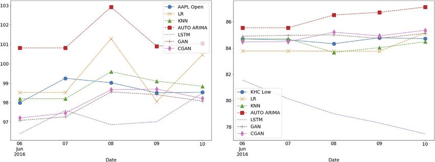
Zhang et al.                                                                                                  Adversarial Learning for Stock Prediction

should also be taken into consideration besides historical                  2 RELATED WORKS
prices. Investors’ sentiments, economic conditions, and
public opinions are all critical variables that should be                   In this section, we first present an overview of the relatively recent
added into a stock prediction system. Particularly, sentiment               generative adversarial networks, followed by a brief review of
analysis has been identified as a useful tool in recent years. Not           some traditional methods for stock price prediction.
just price and price-related values, researchers have paid more
attention to the extraction of sentiment information from                   2.1 Adversarial Learning of Neural Networks
newspapers, magazines, and even social media. For example,                  Generative adversarial networks (GANs) [7], which try to fool a
Ref. [1] examined the relation between social media sentiment               classification model in an adversarial minimax game, have shown
and stock prices, in addition to economic indicators in their               high potential in obtaining more robust results compared to
research on stock market. Ref. [2] Focused on combining                     traditional neural networks [8]. In a GAN framework, a generator
stock-related events with the sentiment information from                    produces fake data based on noisy samples and attempts to
reviews of financial critics. They analyzed sentiments and                   minimize the difference between real and fake distribution,
predicted the fluctuation of the stock market with a matrix                  which is maximized by a discriminator oppositely. The GAN
and tensor factorization framework. Besides mathematical                    framework and GAN-based research have attracted huge
methods, the development of natural language processing                     attention in various fields recently. Existing GAN works
also provides additional techniques for analyzing text and                  mainly focus on computer vision tasks like image classification
sentiment information. Machine learning, data mining, and                   [9] and natural language processing like text analysis [10]. With
semantic comprehension have made extracting large amounts                   the inception and extensive applications of knowledge
of stock sentiments possible. With the development of social                representation of natural or complex data such as languages
media, people are increasingly inclined to exchange                         and multi-media, the GAN framework is also widely applied
information through the Internet platform. Real-time stock                  to classification missions for data in representation spaces (e.g.,
reviews contain a wealth of financial information that reflects               vector spaces of matrices) rather than just for the original data in
the emotional changes of investors. Works such as [3, 4]; and               feature spaces. Some researchers also extended applications of
[5] analyzed sentiment information from large numbers of                    GAN to more challenging problems such as recommendation
real-time tweets, which were related to stocks and                          systems [11] or social network alignment problems [12].
corresponding companies, then investigated the correlation                     Conditional GANs (CGANs) [13] add auxiliary information
between stock movements and public emotions with                            to input data, guiding the training process to acquire expected
supervised machine learning principles. In particular, Ref.                 results. Additional information (like class labels or extra data) is
[3] utilized two mood tracking tools, OpinionFinder and                     fed into both generator and discriminator to perform the
Google-Profile of Mood States (GPOMS), to analyze the text                   conditioning. This architecture is mostly used in image
content of daily tweets, which succeeded in measuring varying               generation [14] and translation [15]. However, we noticed that
degrees of mood. These research results proved that modern                  the CGAN framework has rarely been applied to time-series
techniques are mature enough to handle mountains of                         prediction, specifically, stock prediction problem. In our work, we
sentiment data and that Twitter is a valuable text resource                 added sentiment labels to guide the training process of our model
for sentiment analysis.                                                     and achieved a stronger performance.
    In our work, we used VADER (Valence Aware Dictionary and                   Previous work [16] has shown the capacity of GANs for
sEntiment Reasoner) [6] as a mood tracking tool to help us                  generating sequential data and to fulfill the adversarial training
analyze the sentiment information from tweets. We extracted                 with discrete tokens (e.g., words). Recurrent neural networks
sentiment features from the past several days of tweets and input           (RNNs) have also been widely used to solve problems based on
them into stock prediction models to predict future stock prices.           sequential data, such as speech recognition and image
Applying sentiment analysis to nine stocks, we trained the models           generation. Ref. [17] first combined RNNs with a GAN
with two-month-long training sets with tweets and tested the                framework and successfully produced many kinds of
model performance with the final five days’ data. We applied                  continuous sequential data, including polyphonic music.
several linear and nonlinear models such as LSTM to this                    Inspired by this work, researchers paid more attention to the
regression task. Moreover, referring to the theories of                     potential of RNNs in adversarial training. Refs. [18, 19]
recurrent neural networks and generative adversarial networks,              succeeded in producing realistic real-valued multi-
we designed a sentiment-guided model to improve the accuracy                dimensional time-series data and concentrated their work on
of stock prediction further.                                                medical applications. They built models capable of synthesizing
    In the remainder of this article, the organization is set in the        realistic medical data and developed new approaches to create
following order: First, in Section 2 we review existing stock               predictive systems in the medical domain. Ref. [20] utilized
prediction methods and the development of GANs. Then, in                    prerecorded human motion data to train their models and
Section 3, we introduce our methods in data collection and                  applied their neural network in random motion synthesis,
processing. In Sections 4 and 5, we propose our sentiment-                  online or offline motion control, and motion filtering. Our
guided adversarial learning model as well as comparisons                    work drew on the idea of the RNN-GAN framework and
between our models and baselines. Finally, conclusions and                  applied time-series analysis to the financial problem of stock
future work are discussed at the end of this paper in Section 6.            prediction. Although similar application in stock prediction has

Frontiers in Applied Mathematics and Statistics | www.frontiersin.org   2                                       May 2021 | Volume 7 | Article 601105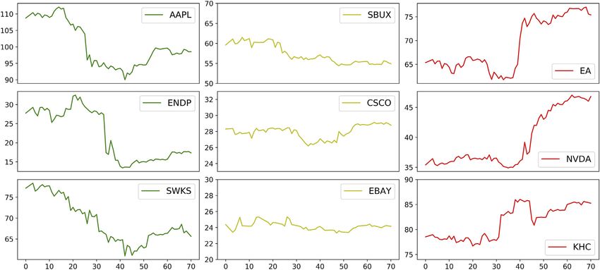
Zhang et al.                                                                                                 Adversarial Learning for Stock Prediction

been raised recently [21], the main difference was that our work            3 DATA AND METHODS
also utilized text data from Twitter to create sentiment scores,
which could gauge the market mood and guide our models to                   In this section, we document our data sources and preprocessing
achieve more accurate prediction.                                           techniques. The latter part includes feature engineering,
                                                                            imputation of missing data, fast Fourier transform for
2.2 Stock Prediction Methods                                                denoising data, and last but not least, Isolation Forest for
The stock market prediction problem has a long history and is               anomaly or outlier detection.
regarded as an essential issue in the field of financial
mathematics. According to the development of research                       3.1 Data Collection and Sentiment Analysis
over the years, we can divide the prediction techniques into                Before we started our work, we had the conviction that a
two categories: statistical and machine learning methods.                   collection of tweets related to the stocks could make
Frequently used statistical techniques include the                          comparatively accurate models of the investors’ mood and
autoregressive method (AR), the moving average model                        thus reach better predictions of the stock market prices.
(MA), the autoregressive moving average model (ARMA),                       Generally speaking, tweets have neutral, positive, or negative
and the autoregressive integrated moving average (ARIMA)                    emotions; and we focused on those that contains one or
[22]. These methods adopt the principles of random processes                several cashtags (unique identifiers for businesses), which
and essentially rely on past values of the sequences to analyze             could influence the stock’s trend in the following day. If
and predict the future data. Another technique is generalized               negative sentiment dominated a day, then the next day’s stock
autoregressive conditional heteroskedasticity (GARCH) [22],                 prices would be expected to fall. The number of followers on one’s
which takes the fluctuation of variance into account and nicely              Twitter account would also be a significant factor. The more
simulates the variation of financial variables. However, both                followers of an account, the higher the influence of tweets from
kinds of techniques depend on strong prerequisites such as                  the account, and the more significant their impact would likely
stationarity and independent and identically distributed (iid)              have on stock prices. Cashtags system is a particularly convenient
random variables, which may not be satisfied by data in the                  feature of Twitter, allowing users to see what everyone is saying
real-world financial markets.                                                about public companies. The way this system works is similar to
   Recently, machine learning methods (including linear                     the well-known #hashtags of Twitter, except that a cashtag
regression, random forest, and support vector machine)                      requires “$” followed by a stock symbol (e.g., $GOOG for
stimulate the interest of financial researchers and are                      Google, LLC; $FB for Facebook, Inc.; and $AAPL for Apple Inc.).
applied to forecasting problems. Among them, support                            For our work, financial tweets and their retweets were
vector machine (SVM) and its application in the financial                    downloaded from the website, https://data.world/kike/nasdaq-
market revealed superior properties compared to other                       100-tweets. The time span of these tweets is 71 days from Apr
individual classification methods [23]. Since the emergence                  1–June 10, 2016. We could get all tweets mentioning any
of deep learning networks, researchers have proved that neural              NASDAQ 100 companies from this source. The key daily
networks can obtain better performance than linear models.                  stock price data includes Open prices (O), High prices (H),
Their capacity to extract features from enormous amount of                  Low prices (L), and Close prices (C); they were subsequently
raw data from diverse sources without prior knowledge of                    crawled from Yahoo Finance with the Python package, pandas_
predictors makes deep learning a preferred technique for stock              datareader. We produced nine datasets, each one including tweets
market prediction. Artificial neural networks and other                      and price values for the nine companies as listed in Table 1. These
advanced neural models like convolution neural networks                     companies are from different sectors/industry groups by the
(CNNs) are evidenced to be good at capturing the non-                       Global Industry Classification Standard (GICS). They could be
linear hidden relationships of stock prices without any                     classified into three price-trend categories: descending prices,
statistical or econometric assumption [24]. Furthermore,                    mildly fluctuating prices, and ascending prices. Figure 1 shows
neural networks have also been found to be more efficient                    the Open price curves of nine stocks with the three distinct trends.
in solving non-linear financial problems compared to                             To analyze the sentiment of each tweet, we used VADER [6],
traditional statistical methods like ARIMA [25]. Nowadays,                  which is available from vader-sentiment, a ready-made Python
RNNs are one of the most popular tools in time-series                       machine learning package for natural language processing.
prediction problems. Notably, the LSTM network has been                     VADER is able to assign sentiment scores to various words
a great success due to its ability to retain recent samples and             and symbols (punctuations), ranging from extremely negative
forget earlier ones [26]. Each LSTM unit has three different                (−1) to extremely positive (+1), with neutral as 0. In this way,
gates: forget gate, update gate, and output gate. LSTM units can            VADER could get an overall sentiment score for a whole sentence
change their states by controlling their inner operant, namely,             by combining different tokens’ scores and analyzing the grammar
their three gates. In our model, we utilized the LSTM network               frames. We assumed that the neutral emotion plays a much
to extract features according to the timeline and to generate               weaker role in the overall market’s mood since neural sentiment
fake stock prices from real past price values. We also used                 tends to regard the stock market as unchanged in a specific
sentiment measures to enhance the robustness of our                         period. Thus, we excluded the neutral sentiment scores in our
prediction models and make the generative results approach                  analysis and only took the negative and positive moods into
the real distribution.                                                      consideration. VADER places emphasis on the recognition of

Frontiers in Applied Mathematics and Statistics | www.frontiersin.org   3                                       May 2021 | Volume 7 | Article 601105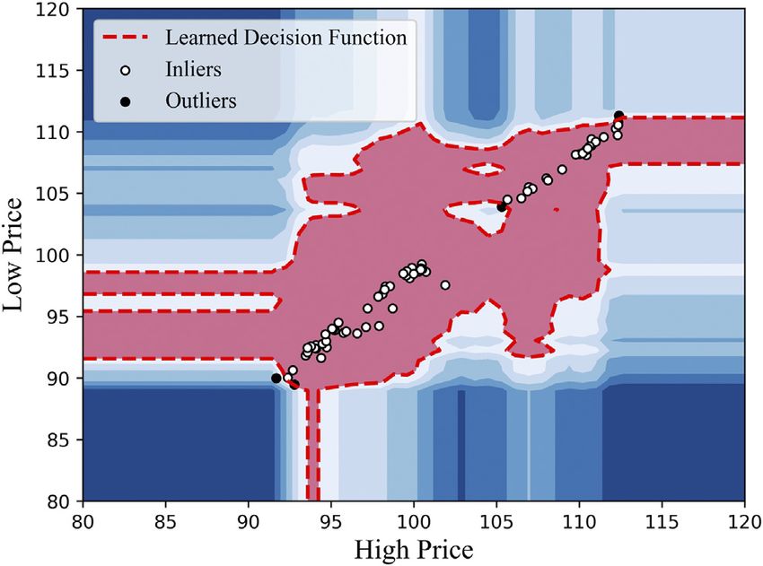
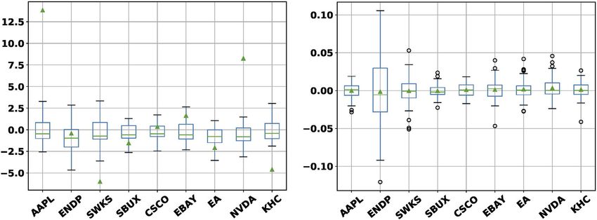
Zhang et al.                                                                                                                      Adversarial Learning for Stock Prediction

TABLE 1 | Stock prices of nine companies selected for experiments in this study.

Company                                           Symbol                                     Sector                                              Industry group

Apple Inc                                         AAPL                               Information Technology                            Technology Hardware & Equipment
Cisco Systems Inc                                 CSCO                               Information Technology                            Communications Equipment
Electronic Arts Inc                               EA                                 Communication Service                             Media & Entertainment
Eastbay Inc                                       EBAY                               Consumer Discretionary                            Internet & Direct Marketing Retail
Endo International PLC                            ENDP                               Health Care                                       Pharmaceuticals
Kandy Hotels Co                                   KHC                                Consumer Discretionary                            Hotels Resorts & Cruise Lines
NVIDIA Corporation                                NVDA                               Information Technology                            Semiconductors
Starbucks                                         SBUX                               Consumer Discretionary                            Consumer Services
Skyworks Solutions Inc.                           SWKS                               Information Technology                            Semiconductors

  FIGURE 1 | The nine stocks classified into three classes with distinct price trends. The variations of Open price from April 1 to June 10, 2016 are displayed. The first
  column presents the stocks with descending prices; the second represents the stocks with mildly fluctuating prices; and the third represents the stocks with ascending
  prices.

uppercase letters, slang, exclamation marks, and the most common                             To get one day’s overall sentiment score for one stock, we first
emojis. Tweet contents are not written academically or formally, so                      analyzed all related tweets with VADER and gained the scores of
VADER is suitable for social media analysis. However, we needed to                       each tweet. Considering that the more followers the bigger
add some new words to the original dictionary of VADER, because                          influence, we further regarded the number of followers as
VADER missed or misestimated some important words in financial                            weights and calculated the weighted average of sentiment
world and therefore caused inaccuracy. For example, “bully” and                          scores. The daily percentage change of this average was taken
“bullish” are negative words in the VADER lexicon, but they are                          as a comprehensive factor, called compound_multiplied, for
positive words in the financial market. We updated the VADER                              1 day. One problem of our data was that we have only tweets’
lexicon with the financial dictionary Loughran-McDonald Financial                         data but no price data on the non-trading days. To make full use
Sentiment Word Lists [27], which include many words used in the                          of the tweets’ data, we filled the gaps up with the price values from
stock market. This dictionary has seven categories, and we adopted                       past trading days. We utilized moving averages to fill in the
the “negative” and “positive” lists. We further deleted about 400                        missing values.
existing words in VADER that overlap the Loughran-McDonald                                   We also normalized the compound_multiplied variable as
Financial Sentiment Word Lists. Finally, we added new negative and                       neural networks generally perform better and more efficiently
positive words to the VADER dictionary and attached sentiment                            on scaled data. Figure 2 shows the box plots of
scores to them, with +1.5 to each positive word and −1.5 to each                         compound_multiplied and per_change (see Section 5.1.2
negative word from the Loughran-McDonald lists.                                          for details) for the nine stocks before the data was scaled.

Frontiers in Applied Mathematics and Statistics | www.frontiersin.org                4                                              May 2021 | Volume 7 | Article 601105
Zhang et al.                                                                                                                  Adversarial Learning for Stock Prediction

  FIGURE 2 | Left: Box plots of changes in daily sentiment scores aggregated from tweets that contained cashtags of selected stocks over the time period Apr
  2–Jun 10, 2016. Outliers are omitted to declutter the graph. The triangles mark the mean values. Right: Box plots of per_change with outliers shown as circles.

                                                                                      using other quantitative indicators. The main steps of
                                                                                      distinguishing outliers were as follows: For a group of data
                                                                                      with multiple dimensions, we attempted to build a binary
                                                                                      search tree (BST). We first picked several dimensions, and
                                                                                      then randomly selected one dimension and a value between
                                                                                      the maximum and the minimum in that dimension as the
                                                                                      root of the BST. Next, we divided the data into two groups
                                                                                      (i.e., subtrees of the BST) according to the selected value.
                                                                                      Likewise, we continued to subdivide the data according to
                                                                                      another randomly selected value in another feature
                                                                                      dimension—this step was repeated until the BST could not be
                                                                                      further subdivided. Finally, we detected the anomaly data
                                                                                      according to the path lengths of the nodes in the BST.
                                                                                          More specifically, in our work, we adopted only two dimensions
                                                                                      in the iForest algorithm and detected the outliers within two steps.
                                                                                      (I) We selected High price and Low price as the two dimensions to
                                                                                      detect anomaly situations that stock prices fluctuated intensely in
  FIGURE 3 | Detecting outliers in the dimensions of High price and Low               one day. Figure 3 shows the anomaly detection results when we
  price with Isolation Forest on AAPL-Open in the training dataset. Only four         applied the iForest to the AAPL dataset. (II) For each one of the four
  points of outliers were flagged out by the algorithm.
                                                                                      price series (O, H, L, C), we respectively selected the differences yt −
                                                                                      yt−1 and yt+1 − yt , in which yt was the price data on a particular date
                                                                                      t, as the two input dimensions to iForest. In this way, we were able to
3.2 Data Processing for Stock Prices                                                  detect anomaly local trends on the timeline. Figure 4A shows the
As discussed before, we collected stock prices from nine stock                        detection result of ‘Open Price’ from the AAPL dataset, and
symbols, each of which contains four columns of time-series price                     Figure 4B displays the anomaly in the form of time series. After
data for each trading day: Open, High, Low, and Close. To change                      we identified each outlier yt by considering its distances from yt ± 1
the sequential data into suitable input for our models, we did data                   using iForest, we replaced yt with the rolling average
                                                                                      3 (yt−2 + yt−1 + yt ). As a result, we prevented our model from
                                                                                      1
cleaning and transformation for the training datasets, and
approximate normalization for our both training and testing                           being excessively influenced by outliers during the training process.
data. We present further details of these transformations below.
                                                                                      3.2.2 Data Transformation
3.2.1 Data Cleaning                                                                   We noticed the successful applications of RNNs in wave forms like
In consideration of the volatility of the stock market, we had to                     sinusoids, so we further transformed our time-series datasets into a
tackle the price data on days that showed abnormal trends or                          wave-like form in order to improve the training effect. In our
fluctuation. To accomplish the anomaly detection, we utilized the                      prediction problem, we assumed that the changes in stock data
Isolation Forest (iForest) algorithm [28] to find such data points                     were periodic, which gave us the opportunity to introduce Fourier
before treating them. Isolation Forest can directly describe the                      Transform into our data processing work. Fourier transform can
degree of isolation of data points based on binary trees without                      decompose a periodic function into a linear combination of

Frontiers in Applied Mathematics and Statistics | www.frontiersin.org             5                                             May 2021 | Volume 7 | Article 601105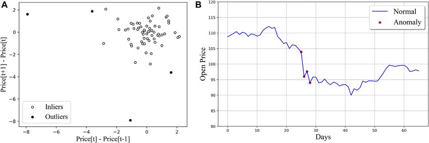
Zhang et al.                                                                                                                        Adversarial Learning for Stock Prediction

  FIGURE 4 | (A) Detecting outliers according to (yt − yt−1 ) and (yt+1 − yt ) with Isolation Forest using the AAPL-Open training set as an illustration. (B) Anomaly
  detection results in the form of time series on the same price values in (A).

  FIGURE 5 | Fourier transform curves with 5, 15, 25, 30, and 32 components on AAPL-Open training set.

orthogonal functions (such as sinusoidal and cosine functions) [29].                      data are iid normal samples, as long as the sequential data has
With Fast Fourier Transform (FFT), we could extract both global and                       constant mean and same variance over time; see [30]; for example.
local trends of our stock datasets and thus reduce their noise. For each                  We calculated Rt , defined as one-period simple returns of the price
of the four prices (O, H, L, C of a stock dataset), we respectively used                  values before inputting them into our supervised learning models as
FFT to create a series of sinusoidal waves (with different amplitudes                     targets, where yt represents one of the four prices for a given stock on
and frames) and then combined these sinusoidal waves to                                   day t that we are interested to predict:
approximate the original curve. In Figure 5, we can see that the                                                                  yt − yt−1
pink curve, which was made by a combination of 32 components,                                                              Rt              .                            (1)
                                                                                                                                     yt−1
closely approximates the original price graph of AAPL-Open training
set. By using the derived curve, namely, the denoised sequential data,                         t be an estimate of Rt returned by a machine learning model
                                                                                          Let R
we could enhance the smoothness of our training set, and reduce                           trained with predictors including historical returns,
noisiness in our data. Consequently, we smoothened the time-series                        Rt−1 , Rt−2 , /, Rs for some s < t. Subsequently, we can obtain an
data to make our training data more predictable.                                                                                        t ).
                                                                                          estimate of the stock price, yt  yt−1 (1 + R

3.2.3 Approximate Normalization
To make sure that our models could learn the features of time-series                      4 MODEL THEORY
variables, we also modified the sequential price data to make it satisfy
(roughly) normal distribution. In financial research, there is a                           In this section, we present the architecture of our CGAN
traditional assumption that the simple daily returns of time-series                       framework in relation to the sub-networks of our choice.

Frontiers in Applied Mathematics and Statistics | www.frontiersin.org                 6                                               May 2021 | Volume 7 | Article 601105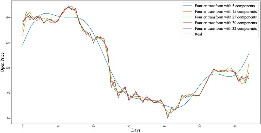
Zhang et al. Adversarial Learning for Stock Prediction
FIGURE 6 | Information flow through an LSTM unit.
4.1 Long Short-Term Memory Networks
Introduced by [31], LSTM is a special kind of RNN, which can learn
both short-term and long-term correlations effectively from
sequential data. An LSTM network usually consists of many
repeating modules, the LSTM units, and we can tune the number
of the units to improve the performance of the network. These
LSTM units concatenate with each other in line with the information
transmitting from one to another. Each unit contains three kinds of
gates: Forget gate (decides what kind of old information to be
discarded), Update gate (decides what kind of new information
to be added), and Output gate (decides what to be output). Figure 6
shows how the past information flows through an LSTM unit
between two time steps, and how the LSTM unit transforms the
data in both its long-term and short-term memory. The information
transmission process is from Ct−1 to Ct , which will be changed by
inner operants. Ct is a latent variable; χ t is the input; and yt is the
output. The mathematical operations in the three gates are defined as
follows, where W. and b. are parameters to be estimated for
minimizing some loss functions:
I. Forget gate:
Ft sigmoidWf yt−1 , χ t + bf . (2)
II. Update gate:
Ut sigmoidWu yt−1 , χ t + bu ,
~ t tanhWC yt−1 , χ + bC ,
C (3)
t
Ct Ft *Ct−1 + Ut *Ct .
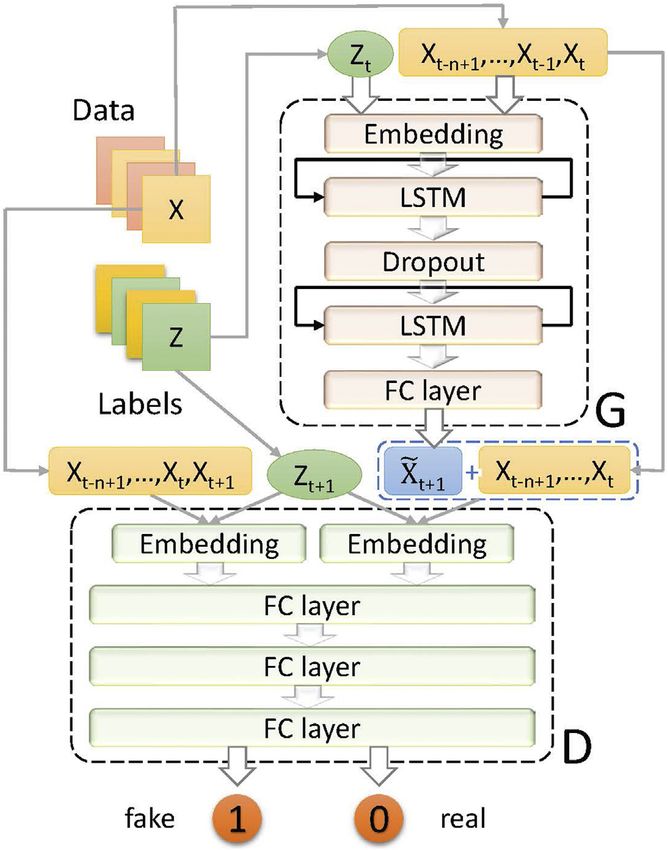
FIGURE 7 | The architecture of our conditional adversarial
III. Output gate: learning model.
Ot sigmoidWo yt−1 , χ t + bo ,
(4)
yt Ot *tanh(Ct ). 4.2 Adversarial Learning Model
As the conditional GAN framework [13] has proved to be a great
Note that sigmoid and tanh are activation functions applied to an success, we adopted this idea in our GAN-based model to
input vector elemenwise, whereas * represents elementwise improve the training effect. Figure 7 illustrates the
multiplication of vectors. These three gates cooperate with each architecture of our GAN-based model. Let Xt
other and together determine the final information that is output {Xt−n+1 , . . . , Xt−1 , Xt } represent the input data in the form of
from an individual unit. In this work, we took advantage of the time series, in which each term is the historical data from the
memory property of LSTM and improved its accuracy with corresponding day from n − 1 days ago to end of current day t.
adversarial learning framework. Note that Xt is a vector that includes all the daily factors on day t.
Nowadays, LSTM has been widely applied in many research In addition, let Zt be the sentiment label on day t. Our generator is
fields such as machine translation, language modeling, and image a multiple-input single-output system, which inputs n historical
generation. days’ data with m factors from the stock market each day (plus,
Frontiers in Applied Mathematics and Statistics | www.frontiersin.org 7 May 2021 | Volume 7 | Article 601105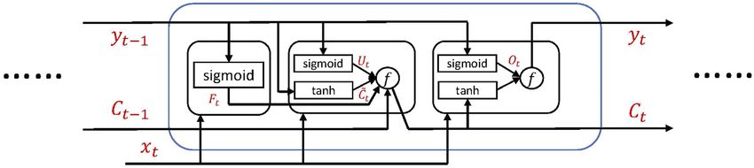
Zhang et al.                                                                                                                Adversarial Learning for Stock Prediction

  FIGURE 8 | Comparison of the prediction curves of different models on the AAPL-Open and KHC Low test sets. For AAPL Open, among all models, KNN achieved
  the minimum MAPE over the five-day test period; see Table 3. However, on each of the last three days, CGAN actually performed better than KNN. For KHC Low, GAN
  predictions were closest to the market values and CGAN came next.

the label) and outputs a specific kind of future price data (Open,                    embedding layers worked in the way same as those in G,
High, Low, or Close) as the prediction. Since the stock data is                      i.e., the embedding layers transformed the data and labels into
typical time-series data, we adopted an LSTM network in our                          suitable input for MLP. The MLP model then projected the data
generative model denoted by G. LSTM was trained to extract the                       into higher dimensional space and effectively accomplished the
features of price data from the past n days, and then used to                        classification task. The Leaky ReLU activation function was used
predict stock prices on day t + 1. The generator model G generally                   in the hidden layers of the MLP and the sigmoid function was
consists of three kinds of layers: embedding layer, LSTM layer,                      used in the output layer. Returning either 0 and class 1, the output
and fully connected (FC) layer. An embedding layer first embeds                       of a discriminator while making a correct decision is as follows:
a label in the latent space and turns it into a dense vector, then
                                                                                                                  0  D(Xt+1 |Zt ),                            (6a)
combines the latent vector with the input matrix, which is the
price data from the past in our application. Afterward, an LSTM                                                         ~ t+1 Zt .
                                                                                                                  1  DX                                      (6b)
layer generates some prediction result. A dropout layer could be
added between two LSTM layers to make the network have a                             Specifically, if we select Open price to be predicted by G, we would
better generalization and less likely to overfit. Lastly, an FC layer                 concatenate the prediction result to Open price values from the
with the Leaky Rectified Linear Unit (ReLU) activation function                       past n days. Then, we distinguished this sequence from the
outputs simulated or fake data X  ~ t+1 , which approximates the real                corresponding one sampled from real data with D.
target data Xt+1 . The output of our generator is defined as follows:                     We alternatively trained G and D with binary cross-entropy
                                                                                     loss (i.e., log loss), L(~y, y)  −y log(~y) − (1 − y)log(1 − ~y), where
                             ~ t+1  G(Xt | Zt ).
                             X                                             (5)       y is the target value and ~y is a predicted value. On the one hand,
                                                                                     our generator G simulated the fluctuations of the stock market
In our work, m  4 and n  5. The four factors were historical                       and to minimize the difference between its prediction and the real
Open price, High price, Low price and Close price, which could be                    data. On the other hand, our discriminator D tried to distinguish
seen as four features of the stock data for the price prediction                     and maximize that difference. The training of G focused on
problem. Specifically, we utilized all four kinds of stock prices in                  making the discriminator D confused; it attempted to
the past five business days to forecast each kind of price (O, H, L,                  minimize the adversarial loss so that D could not discriminate
or C) on the next day.                                                               the prediction easily. The adversarial loss at each data point on
   The purpose of our discriminator D is to classify input data as                   day t + 1 for the generator was
real or fake. This classification model is expected to output 0
when it receives real input data or 1 when it receives fake input                                               ~ t+1   LDX
                                                                                                         Gloss X             ~ t+1 Zt , 0.                      (7)
data. For the input, we concatenated Xt with X            ~ t+1 and Xt+1
                                        ~
respectively to get the fake data X t+1  {Xt−n+1 , . . . , Xt , X ~ t+1 }           The training of D focused on improving its ability to distinguish
and the real data Xt+1  {Xt−n+1 , . . . , Xt , Xt+1 }. In this way, we              the difference between Xt+1 and X   ~ t+1 , so it attempted to
could make the discriminator learn the features of sequential data                   maximize the adversarial loss at each data point on day t + 1:
better. Our discriminator D consists of two parts: two embedding
layers and a multilayer perceptron (MLP) network. The                                                 ~ t+1   L(D(Xt+1 |Zt ), 0) + LDX
                                                                                        Dloss Xt+1 , X                                  ~ t+1 Zt , 1.           (8)

Frontiers in Applied Mathematics and Statistics | www.frontiersin.org            8                                            May 2021 | Volume 7 | Article 601105
Zhang et al. Adversarial Learning for Stock Prediction
In general, the generator tried to make D(X ~ t+1 Zt ) 0 while the matrix of order the same as number of independent
discriminator tried to achieve D(Xt+1 |Zt ) 0 and D(X ~ t+1 Zt ) 1. observations in Y.
[7] defined the loss function of this specific binary classification task K-Nearest Neighbors (KNN) [35] can be used in both
as cross-entropy loss. To achieve the training process described by classification and regression problems. In our time-series
Eq. (7) and Eq. (8), we updated D by maximizing regression problem, the input is the k closest training
Ex ∼ preal (x)[logD(x|z)] + E~x ∼ pfake (~x)[log(1 − D(G(~x|z)))], and then sequences from the feature space according to the timeline,
updated G by minimizing E~x ∼ pfake (~x)[log(1 − D(G(~x|z)))]. In this and the output is the average of the values of the k nearest
way, the total loss function of the minimax game over all training neighbors.
samples was as follows: Autoregressive Integrated Moving Average (ARIMA) is
composed of autoregression (AR), an integrated (I) model that
min maxLRMSprop (D, G) Ex ∼ preal (x) logD(x|z) calculates differences, and moving average (MA). Auto ARIMA
G D
+ E~x ∼ pfake (~x) log(1 − D(G(~x|z))) , [36, 37] can automatically perform grid search with parallel
processing to find an optimal combination of p, q, and d,
(9) which are the parameters associated with order of AR, degree
where preal (x) was the distribution of real data, pfake (~x) was the of differencing with I, and order of MA, respectively.
distribution of fake data, and lastly, z represented the label vector. Long Short-Term Memory is a special kind of recurrent neural
The two models G and D were trained iteratively with the network. We tuned three hyper-parameters to improve its
RMSprop optimizer, a stochastic gradient descent algorithm with training effect: the number of LSTM units, step size, and
mini batches [32]. In each iteration, we first trained the training epochs.
discriminator r times and then trained the generator one time,
in which r was seen as a hyper-parameter to be tuned in our 5.1.2 Data Pre-Processing Techniques
training process. The reason for training D first was that a trained Besides Open price, High price, Low price, and Close price,
discriminator would help improve the training effect of the we also added two more engineered factors to the dataset
generator. Besides, we also adopted gradient clipping (ensuring as input to predict the price on day t + 1. One was the
the norm of a gradient not too large in magnitude) for both G and sentiment variable, compound_multiplied, which was obtained
D at the end of each iteration to avoid the potential problem of with the method illustrated in Section 3.1. The other was
gradient explosion. per_change, which was obtained by the equation:
If Zt is omitted from the discussion in this subsection, then we per change : 100% × [Close(t) − Open(t)]/Open(t). Table 2
have simply a GAN model. In practice, we used Keras [33] with shows the AAPL dataset sample with six columns, where the
TensorFlow [34] version 2 as the backend to implement our compound_multiplied was the sentiment variable.
LSTM, GAN, and CGAN models. Transformations for baseline models (LMR, KNN, and auto
ARIMA) When predicting one type of stock price mentioned
above, we utilized the two derived factors, per_change and
5 EXPERIMENT compound_multiplied, as predictors.
Techniques for neural-network models (LSTM, GAN, and
In this section, we summarize the numerical results of our CGAN) (I) As for LSTM, we chose only three factors as input. For
learning and prediction models in multiple error measures in instance, we used ‘Open price’, per_change and
response to hyperparameter search when applicable. compound_multiplied from day t as input when we predicted
the Open price on day t + 1. However, for our adversarial learning
5.1 Experimental Settings model, we chose four kinds of prices as input and utilized the
We collected price data and related tweets of nine companies other two factors to create labels. The details about the labels were
from April 1st to June 10th, 2016. The data before June 5th was discussed below. (II) We converted time-series data to data that
taken as the training set and the last five days’ data as the test was fitting in supervised learning problems. Specifically, if we
set. For each dataset, we respectively experimented on Open predicted the price on day t + 1 with the prices from the past
price, High price, Low price, and Close price, so we totally built 5 days, we would create a six-term sequence
and tested 9 × 4 36 models and datasets (36 groups of Xt+1 {xt−4 , xt−3 , xt−2 , xt−1 , xt , xt+1 }. In other words, we used
experiments). the first five time-lagged columns as input and the last column
We have already illustrated the main data processing work in as the real target price on day t + 1.
Section 3. Here, we elaborate on specific configuration of our
models. 5.1.3 Settings for Adversarial Learning Models
Labels We utilized the two variables, compound_multiplied and
5.1.1 Baseline Models per_change, to create our final sentiment label in the CGAN
Linear Multiple Regression (LMR) is a classical statistical models. The reason for adding the per_change was that we would
approach for analyzing the relationship between one like to take the local trend of past stock variation into account.
dependent variable and one or more independent variables. Its Finally, the label was set to three classes: 0, 1, and 2. The three
simple formula in matrix notation is Y Xβ + ε, where ε is iid classes respectively represent three different tendencies of
normal with mean 0 and variance matrix, σ 2 I, and I is the identity forecasting prices: up, down, and almost unchanged. Our
Frontiers in Applied Mathematics and Statistics | www.frontiersin.org 9 May 2021 | Volume 7 | Article 601105Zhang et al. Adversarial Learning for Stock Prediction
TABLE 2 | Stock price data and two engineered features on the first five days of the AAPL dataset, where NaN represents Not a Number.
Date Open High Low Close per_change compound_multiplied
4/1/16 108.78 110.00 108.20 109.99 1.1123 NaN
4/2/16 109.33 110.73 108.89 110.37 0.9529 1.1750
4/3/16 109.87 111.46 109.58 110.74 0.7934 -0.1666
4/4/16 110.42 112.19 110.27 111.12 0.6339 -0.1836
4/5/16 109.51 110.73 109.42 109.81 0.2739 0.2064
model was trained to learn the categories from labels with the the learning rates of the sub-networks, αD and αG ; the epoch
training set and enhance its prediction accuracy. Let Zt represent ratio r; weightage λ1 and λ2 in Eq. (10). Table 3 show the MAPE
the label on day t. The process of creating the labels could be results of the nine test sets. We did four groups of experiments,
captured by the following min-max scaling of each vt ∈ [0, 3] respectively on O, H, L, C, for each test set and then calculated the
before mapping it to Zt ∈ {0, 1, 2}, meaning [0, 1) 1 0, [1, 2) 1 average MAPE to compare the performances of different models
1, and [2, 3]12: effectively. KNN achieved minimum mean MAPE for AAPL,
SBUX, CSCO, SWKS, and KHC; linear models for EA and ENDP;
vt λ1 × compound multiplied(t) + λ2 × per change(t), (10)
GAN and CGAN for NVDA and EBAY, respectively. While KNN
vt − min(vt ) achieved minimum errors most of the time, GAN and CGAN
Zt min 2, 3 ,
max(vt ) − min(vt ) were the best for 11 of the 36 stock prices and the second best for
18. In terms of overall average of all nine MAPEs (last column of
where λ1 + λ2 1 and 0 ≤ λ2 , λ2 ≤ 1. Empirically, tuning λ1 and λ2 Table 4), KNN was the best and CGAN came as a close second.
could change the training accuracies. Without sentiment labels, GAN models on average had a higher
We also did experiments to evaluate the impact of the average of all MAPEs than CGAN, showing that our sentiment
sentiment analysis had made in our work. Specially, we labels help generally in improving price prediction accuracy.
modified our CGAN models by taking out the embedding Root mean square errors (RMSE), mean square errors (MSE),
layers and not inputting the sentiment labels Zt . Without the mean absolute errors (MAE), and symmetric mean absolute
labels Zt, we have GAN models. In this way, we could compare the percentage errors (SMAPE) were also used to verify the
training effect of our models with or without sentiment labels. training results. Their defining equations are recapped here:
Hyper-parameters As discussed in Section 4, we alternately
trained the D and the G. The epoch ratio, r, defined as epochs of D
to epochs of G, was in the range of [1, 4]. 1 N 2 1 N 2
RMSE yt − ~yt , MSE yt − ~yt ,
The learning rates for D and G, αD and αG , were searched in the N t1 N t1
range, [5 × 10− 5 , 8 × 10− 4 ], respectively, with the same decay, 10−8.
We also tuned αD and αG in our experiments to improve the training 1 N 100% N yt − ~yt
MAE |yt − ~yt |, SMAPE .
process. Besides, the gradient clipping thresholds were set to be the N t1 N t1 yt + ~yt 2
same at 0.8 for both the generator and the discriminator.
To evaluate our model in a more comprehensive view, we selected
5.2 Results and Discussions AAPL and EBAY to illustrate these four metrics. We respectively
We used mean absolute percentage errors (MAPE) as the main obtained the results of O, H, L, C from all models and then
metric to evaluate the performance of our model. The metric calculate the average errors to compare the performance more
equation is carefully. Table 5 for AAPL shows that KNN performed best on
average while CGAN came second. Table 5 for EBAY
100% N yt − ~yt demonstrates that the CGAN models outperformed all the
MAPE ,
N t1 yt baselines not only in MAPE but also in RMSE, MSE, MAE,
and SMAPE.
where yt is the real price on day t, ~yt is the prediction price by a As discussed above, we treated λ1 and λ2 as hyper-parameters.
model, and N is number of data points. In our experiments, we first Considering the importance of condition labels, adjusting the
trained the CGAN model until the loss curves of both the generator and proportion of sentiment information would be necessary every
the discriminator converged. The training process was described in time we trained the CGAN model. For short-term stock data,
Section 4. After that, we tested the generator “LSTM model” to get the we need to train the model only once, since people’s attitude
prediction results of testing data. Figure 8 displays the comparison of toward a stock often remains more or less the same in a short
prediction curves on the AAPL-Open and KHC-Low test sets. As our period. However, readjusting λ1 and λ2 every month maybe
test sets contained five-day-long data, we calculated the average MAPEs useful. We collected another tweet dataset about Apple Inc.
for the five days’ OHLC prices as the performance metric of the model. with a time span from Jan. 1, 2014 to Dec. 31, 2015 (available
Empirically, we tuned three kinds of hyper-parameters to from stocknet-dataset by [5]. We selected three periods in these
improve the performance of our adversarial learning model: two-year-long datasets and calculated the MAPEs of prediction
Frontiers in Applied Mathematics and Statistics | www.frontiersin.org 10 May 2021 | Volume 7 | Article 601105Zhang et al. Adversarial Learning for Stock Prediction
TABLE 3 | Tables 3a–i present the MAPEs of forecasted O, H, L, and C prices from TABLE 3 | (Continued) Tables 3a–i present the MAPEs of forecasted O, H, L, and C
various models for nine stock symbols. The smallest MAPE is highlighted in prices from various models for nine stock symbols. The smallest MAPE is highlighted
bold across the models in each column for every stock price; the second smallest in bold across the models in each column for every stock price; the second smallest
is underlined. The last column contains the average values of the MAPEs of the is underlined. The last column contains the average values of the MAPEs of the four
four price targets. price targets.
Open High Low Close Mean/% Open High Low Close Mean/%
a). MAPEs of the AAPL test set. LSTM 0.8691 5.9214 6.3042 5.9614 4.7640
LMR 1.1958 2.9199 1.4223 2.1880 1.9315 GAN 0.5725 0.2316 0.3953 0.7931 0.4981
KNN 0.5546 0.8539 0.4884 0.4090 0.5765 CGAN 0.5304 0.3763 0.4749 0.6463 0.5070
ARIMA 2.6741 1.4260 3.2027 2.6597 2.4906
LSTM 1.4061 4.5924 5.7139 5.2507 4.2408
GAN 0.7929 1.5085 1.2227 1.2868 1.2027
CGAN 0.7067 1.4688 0.6841 1.3076 1.0418
TABLE 4 | Counts number of times a model is the best and second best in
b). MAPEs of the SBUX test set.
predicting the stock prices, and lists the mean of all mean values in the last
LMR 0.9019 1.1674 1.3397 1.2923 1.1753
column of Tables 3a–i.
KNN 0.5593 0.4919 0.6338 0.5265 0.5529
ARIMA 1.1861 1.0757 1.1539 1.0580 1.1184 Overall performance of all models
LSTM 0.5040 3.8398 4.0186 3.7970 3.0399
GAN 0.6448 0.8664 0.8240 0.9556 0.8227 Best Second Mean/%
CGAN 0.6888 0.9053 0.6280 0.8969 0.7798
c). MAPEs of the EA test set. LMR 6 4 1.5026
LMR 0.5037 0.8308 0.9628 0.9709 0.8170 KNN 14 12 0.9965
KNN 0.5964 0.8414 0.9878 1.0162 0.8604 ARIMA 0 1 2.7738
ARIMA 3.1441 3.8026 1.4712 2.4455 2.7158 LSTM 5 1 7.8412
LSTM 0.8987 16.9632 17.0647 16.4948 12.8554 GAN 8 8 2.6033
GAN 0.9095 0.8225 1.0935 0.7298 0.8888 CGAN 3 10 1.3035
CGAN 1.2390 1.0105 1.3181 0.7448 1.0781
d). MAPEs of the ENDP test set.
LMR 2.6631 2.892 3.2137 2.8585 2.9068
KNN 2.4014 2.4446 4.3038 3.4666 3.1541
TABLE 5 | Comparison of prediction results in different metrics on the AAPL and
ARIMA 7.5329 10.8514 7.8179 12.4049 9.6518
EBAY test sets using the average values of model errors on O, H, L, C prices.
LSTM 1.9243 33.3106 27.6254 37.3947 25.0638
The smallest errors are displayed in bold font across the models we have built; the
GAN 3.4240 53.2661 3.9620 4.8264 16.3696
second smallest errors are underlined.
CGAN 5.4597 3.6090 4.0107 3.1991 4.0696
e). MAPEs of the CSCO test set. Model RMSE MSE MAE MAPE/% SMAPE/%
LMR 1.1367 0.6497 0.8273 0.4343 0.7620
KNN 0.3813 0.1555 0.7219 0.1840 0.3607 a). Errors of the AAPL test set.
ARIMA 1.3303 1.7011 2.7049 1.1942 1.7326 LMR 2.2721 5.8504 1.9176 1.9315 1.9231
LSTM 0.5645 7.2849 7.9551 8.0766 5.9703 KNN 0.7154 0.5680 0.5721 0.5764 0.5753
GAN 0.4081 0.2811 0.6025 0.2095 0.3753 ARIMA 2.6184 7.1359 2.4613 2.4906 2.4546
CGAN 0.6318 0.4245 0.6968 0.2559 0.5022 LSTM 5.1174 30.7145 4.2006 4.2408 4.1406
f). MAPEs of the NVDA test set. GAN 1.5321 2.5507 1.1970 1.2028 1.2152
LMR 2.4894 2.5058 2.0899 3.6247 2.6774 CGAN 1.3464 2.0495 1.0378 1.0418 1.0511
KNN 0.9341 1.0531 0.6399 1.5637 1.0477 b). Errors of the EBAY test set.
ARIMA 2.1786 1.9938 1.5984 2.0929 1.9659 LMR 0.2457 0.0689 0.1994 0.8234 0.8287
LSTM 0.8402 12.1243 10.8188 10.297 8.5201 KNN 0.1970 0.0392 0.1628 0.6735 0.6765
GAN 1.0658 0.7822 0.4776 1.2834 0.9022 ARIMA 0.4410 0.2071 0.3453 1.4306 1.4142
CGAN 1.1604 2.4538 0.4854 1.4711 1.3927 LSTM 0.2248 0.0617 0.1636 0.6784 0.6737
g). MAPEs of the SWKS test set. GAN 0.1903 0.0369 0.1534 0.6351 0.6368
LMR 1.3381 1.6378 1.2815 1.6442 1.4754 CGAN 0.1867 0.0353 0.1503 0.6229 0.6230
KNN 1.5065 1.1174 1.2586 1.6564 1.3847
ARIMA 2.5976 2.0430 2.5419 3.4855 2.6670
LSTM 1.9081 6.2990 6.3457 7.1987 5.4379
GAN 1.9350 1.7313 1.2501 2.0234 1.7350 results for the Open price. In the three groups of experiments, we
CGAN 1.7149 1.8520 1.2180 2.1641 1.7372 chose three different (λ1 , λ2 ) pairs in our CGAN model with
h). MAPEs of the EBAY test set. λ2 : 1 − λ1 . We also applied GAN as the baseline to highlight
LMR 0.3222 1.0901 0.813 1.0681 0.8234 the influence of condition labels. As shown in Table 6, for the first test
KNN 0.8402 0.5033 0.6336 0.7170 0.6735
ARIMA 1.1214 1.3163 1.5132 1.7715 1.4306
period, which follows immediately after the time span of the training
LSTM 0.2329 1.2547 0.5792 0.6469 0.6784 data, the MAPEs from CGAN and GAN were least (see the first row
GAN 0.6034 0.5628 0.7878 0.5867 0.6352 of each group in Table 6). However, both models performed worse
CGAN 0.5781 0.4940 0.7231 0.6964 0.6229 with increasingly larger MAPEs during the subsequent test periods
i). MAPEs of the KHC test set.
except for GAN in the last training scenario. Thus, the learning
LMR 0.7283 0.7682 0.8998 1.4204 0.9542
KNN 0.3715 0.1547 0.4089 0.4968 0.3580
models should be trained periodically, or whenever the test errors are
ARIMA 1.0659 1.0437 1.9594 0.6984 1.1919 larger than user-desired tolerances, especially when they are used in
(Continued in next column) real-time prediction tasks.
Frontiers in Applied Mathematics and Statistics | www.frontiersin.org 11 May 2021 | Volume 7 | Article 601105Zhang et al. Adversarial Learning for Stock Prediction
TABLE 6 | Comparison of the MAPEs for AAPL-Open dataset from CGAN and GAN over three different testing periods for each training time span. The smallest error in each
test group for each model is highlighted in bold.
Time span for training set Time span for testing set λ1 CGAN/% GAN/%
2014-01-01–2014-03-31 2014-04-01–2014-04-10 0.2 3.81 3.73
2014-04-11–2014-04-20 5.52 4.93
2014-05-01–2014-05-10 3.88 3.77
2014-07-01–2014-09-30 2014-10-01–2014-10-10 0.2 0.77 0.71
2014-10-11–2014-10-20 1.03 0.97
2014-11-01–2014-11-10 0.95 0.88
2015-01-01–2015-03-31 2015-04-01–2015-04-10 0.9 2.90 8.98
2015-04-11–2015-04-20 9.58 8.71
2015-05-01–2015-05-10 10.65 9.79
6 CONCLUSIONS AND FUTURE WORK complicated and there are potentially a great many factors to be
considered. There are some other factors like economic growth,
For individual investors and investment banks, rational prediction interest rates, stability, investor confidence and expectations. We
through statistical modeling helps decide stock trading schemes also noticed that political events would have a huge impact on the
and increase their expected profits. However, it is well known that variation of the stock market. We can extract political
human trading decisions are not purely rational and the irrational information from newspapers and news websites. If we added
drivers are often hard to observe. Introducing proxies of irrational these factors to the input, our model may better learn the features
decision factors such as relevant online discussion from Twitter of the stock market and make the prediction tendencies close to
followed by sentiment analysis has become an advanced approach that in the real world.
in financial price modeling. In this work, we have assumed that the tweets are more or
In this work, we have successfully built a sentiment- less truthful. However, social media sources could be
conditional GAN network in which LSTM served as the contaminated with fake news or groundless comments, that
generator. We encoded Twitter messages, extracted sentiment are hard to be distinguished from the good ones with real
information from the tweets, and utilized it to conduct our stock signals. A fruitful area of future research is to look into GAN
prediction experiments. The experiments showed, for about a models for alleviating the problem.
third of our models, superior properties of our GAN and CGAN It is also known that neural network models often need
models compared to LMR and ARIMA models, KNN method, much bigger datasets to beat simpler models. To this end, there
as well as LSTM networks. Our GAN and CGAN models could are multiple ways we could explore: consider more than nine
better adapt to the variations in the stock market and fluctuation stocks; join all stock prices into one single dataset, i.e., to train
trends of some real price data. Hence they could play a role in one model on panel data grouped by stocks and prices (O, H, L,
ensemble methods that combine strong models with small C) instead of a single time series; sample our datasets at hourly
prediction errors to achieve better accuracies than any frequency.
individual model when no one model would always perform Lastly, many properties of neural networks are still active areas of
best; see, for example, [38]. research. For example, in LSTM, GAN, and CGAN models, the loss
Even though our neural network models could outperform the function values and the solution quality often appear to be sensitive
simpler baseline models at times, it could still be enhanced. The main to small changes in inputs, hyperparameters, or stopping conditions.
obstacle in our work was that we failed to find tweets’ dataset that Creating stable yet efficient numerical algorithms are necessary for
was longer than 70 days, which might largely weaken the training reliable solutions. In addition, the success of neural networks are
effect. For instance, we initially planned to add more labels to our often associated with computer vision problems. Adopting them in
input data, since it would help represent varying degrees of finance may require different techniques or transformations.
sentiment tendencies instead of only ‘up’, ‘down’, and ‘almost In the future, we would like to explore the topic further in the
unchanged’. Nevertheless, the GAN-based models could not learn following directions:
better with more labels in such a short time-series dataset. Therefore,
we finally chose only three classes to make sure that our model 1) Obtaining larger datasets and creating labels in more
would be fully trained. The same consideration went when we classes to improve our model by examining hourly data,
created the sentiment variable, which was the reason why we for example.
only selected ‘positive’ and ‘negative’ lists when adding new 2) Building GAN models for detecting overhyped or deceitful
words to the dictionary. If we could get a dataset with a longer messages about a stock before incorporating them into our
time coverage, we would be able to do experiments with sentiment models.
labels in more categories and potentially further improve our 3) Attempting to extract more stock-related factors and
models. adding them as predictors in our models.
Another shortcoming in our current approach is that we only 4) Experimenting with more stocks or other financial assets,
took sentiment factors into account. The stock market is very and considering having one model for all stock price data.
Frontiers in Applied Mathematics and Statistics | www.frontiersin.org 12 May 2021 | Volume 7 | Article 601105Zhang et al. Adversarial Learning for Stock Prediction
5) Utilizing more sophisticated natural-language processing code for computational scalability and reproducibility; edited
(NLP) methods to analyze the financial or political manuscript for content accuracy and clarity.
information from news media and assessing the impact
and the role they play in the stock market.
ACKNOWLEDGMENTS
DATA AVAILABILITY STATEMENT The authors would like to thank the editor, Prof. Qingtang
Jiang, and reviewers, Prof. Qi Ye and Prof. Qiang Wu, for their
Publicly available datasets were analyzed in this study. This invaluable support and feedback during the anonymous
data can be found here: https://data.world/kike/nasdaq-100- review process. In addition, we are grateful to the following
tweets. seminar speakers for inspiration during the development of
this work in the 2019 IIT Elevate Summer Program’s research
course, SCI 498-106 Machine Learning Algorithms on
AUTHOR CONTRIBUTIONS Heterogeneous Big Data: Victoria Belotti, Adam Ginensky,
Joshua Herman, Rebecca Jones, Sunit Kajarekar, Hongxuan
YZ: Drafted the manuscript; developed code for data Liu, Lawrence K. H. Ma, Qiao Qiao, Jagadeeswaran
preprocessing and sentiment analysis; designed modeling Rathinavel, Aleksei Sorokin, Huayang (Charlie) Xie, and
methods and experiments. JL: Modified the manuscript and Zhenghao Zhao. In addition, the last author would like to
cooperated in the design of data processing. HW: Modified the thank the following colleagues for discussion and encouragement:
manuscript and cooperated in the design of sentiment analysis. Prof. Robert Ellis, Prof. Robert Jarrow, Jackson Kwan, Wilson
S-CC: Provided directions and supervision on scientific principles Lee, Prof. Xiaofan Li, Prof. Lek-Heng Lim, Aleksei Sorokin, Don
and methodology for the whole project; reviewed and modified van Deventer, and Martin Zorn.
Research & Development in Information Retrieval; 2008 June. New York,
REFERENCES US: ACM (2018) p. 355–64.
12. Li C, Wang S, Wang Y, Yu P, Liang Y, and Liu Y. Adversarial learning for
1. Devi KN, and Bhaskaran VM. Impact of social media sentiments and weakly-supervised social network alignment. In: Proceedings of the AAAI
economic indicators in stock market prediction. Int J Comput Sci Eng Conference on Artificial Intelligence; 2019 Jan 27-Feb 1; Honolulu, Hawaii.
Technol (2015) 6. Menlo park, California: AAAI (2019) 33:996–1003. doi:10.1609/aaai.v33i01.
2. Zhang X, Zhang Y, Wang S, Yao Y, Fang B, and Yu PS. Improving stock market 3301996
prediction via heterogeneous information fusion. Knowledge-Based Syst (2018) 13. Mirza M, and Osindero S. Conditional generative adversarial nets. CoRR abs/
143:236–47. doi:10.1016/j.knosys.2017.12.025 1411.1784 (2014). Available from: http://arxiv.org/abs/1411.1784
3. Bollen J, Mao H, and Zeng X. Twitter mood predicts the stock market. 14. Antipov G, Baccouche M, and Dugelay JL. Face aging with conditional
J Comput Sci (2011) 2:1–8. doi:10.1016/j.jocs.2010.12.007 generative adversarial networks. In: IEEE International Conference on
4. Pagolu VS, Reddy KN, Panda G, and Majhi B. Sentiment analysis of Twitter Image Processing (ICIP); 2017 Sept 17–20; Beijing, China. New York,
data for predicting stock market movements. In: International Conference US: IEEE (2017) p. 2089–93.
on Signal Processing, Communication, Power and Embedded System 15. Yang Z, Chen W, Wang F, and Xu B. Improving neural machine translation
(SCOPES); 2016 Oct 3–5; Paralakhemundi, India. New York, US: IEEE with conditional sequence generative adversarial nets. CoRR abs/1703.04887
(2016) p. 1345–50. (2017). Available from: http://arxiv.org/abs/1703.04887
5. Xu Y, and Cohen SB. Stock movement prediction from tweets and historical prices. 16. Yu L, Zhang W, Wang J, and Yu Y. SeqGAN: Sequence generative adversarial
In Proceedings of the 56th annual meeting of the association for computational nets with policy gradient. In: Thirty-First AAAI conference on artificial
linguistics (Vol. 1: Long Papers); 2018 July; Melbourne, Australia. Stroudsburg, intelligence. New York, US: ACM (2017) 2852–8.
Pennsylvania: Association for Computational Linguistics (2018) 1970–9. 17. Mogren O. C-RNN-GAN: Continuous recurrent neural networks with
6. Hutto CJ, and Gilbert E. VADER: A parsimonious rule-based model for sentiment adversarial training. Constructive Machine Learning Workshop at NIPS
analysis of social media text. In Eighth International AAAI Conference on Weblogs 2016 in Barcelona, Spain. Available from: https://arxiv.org/pdf/1611.09904.
and Social Media; 2014 June 1-4; Ann Arbor, MI. The AAAI Press (2014). 18. Esteban C, Hyland SL, and Rätsch G. Real-valued (medical) time series generation
7. Goodfellow I, Pouget-Abadie J, Mirza M, Xu B, Warde-Farley D, and Ozair S. with recurrent conditional GANs. CoRR (2017). Available from: http://arxiv.org/
Generative adversarial nets. Adv Neural Inf Process Syst (2014) 2672–80. abs/1706.02633.
8. Goodfellow IJ, Shlens J, and Szegedy C. Explaining and harnessing adversarial 19. Zhu F, Ye F, Fu Y, Liu Q, and Shen B. Electrocardiogram generation with a
examples. In: Bengio A, LeCun Y, editors. 3rd International Conference on bidirectional LSTM-CNN generative adversarial network. Sci Rep (2019) 9:
Learning Representations, {ICLR} 2015; 2015 May 7–9; San Diego, CA (2015). 6734. doi:10.1038/s41598-019-42516-z
Available from: http://arxiv.org/abs/1412.6572. 20. Wang Z, Chai J, and Xia S. Combining recurrent neural networks and adversarial
9. Kurakin A, Goodfellow I, and Bengio S. (2017) Adversarial Machine Learning at training for human motion synthesis and control. IEEE Trans Visualization
Scale, 5th International Conference on Learning Representations, ICLR 2017, Comput Graphics (2019) 27:14–28. doi:10.1109/TVCG.2019.2938520
Conference Track Proceedings, Toulon, France, Apr 24–26, 2017, 21. Zhou X, Pan Z, Hu G, Tang S, and Zhao C. Stock market prediction on high-
OpenReview.net. Available from: https://openreview.net/forum?idBJm4T4Kgx frequency data using generative adversarial nets. Math Probl Eng (2018) 2018:
10. Miyato T, Dai AM, and Goodfellow I. Adversarial Training Methods for Semi- 1–11. doi:10.1155/2018/4907423
Supervised Text Classification, 5th International Conference on Learning 22. Wang JJ, Wang JZ, Zhang ZG, and Guo SP. Stock index forecasting based
Representations, ICLR 2017, Conference Track Proceedings Toulon, on a hybrid model. Omega (2012) 40:758–66. doi:10.1016/j.omega.2011.
France, Apr 24–26, 2017, OpenReview.net. Available from: https://arxiv. 07.008
org/abs/1605.07725 23. Huang W, Nakamori Y, and Wang S-Y. Forecasting stock market movement
11. He X, He Z, Du X, and Chua TS. Adversarial personalized ranking for direction with support vector machine. Comput Operations Res (2005) 32:
recommendation. In: The 41st International ACM SIGIR Conference on 2513–22. doi:10.1016/j.cor.2004.03.016
Frontiers in Applied Mathematics and Statistics | www.frontiersin.org 13 May 2021 | Volume 7 | Article 601105You can also read