Global marine gravity from retracked Geosat and ERS-1 altimetry: Ridge segmentation versus spreading rate
←
→
Page content transcription
If your browser does not render page correctly, please read the page content below
JOURNAL OF GEOPHYSICAL RESEARCH, VOL. 114, B01411, doi:10.1029/2008JB006008, 2009
  Click
  Here
    for
 Full
Article

Global marine gravity from retracked Geosat and ERS-1 altimetry:
Ridge segmentation versus spreading rate
David T. Sandwell1 and Walter H. F. Smith2
Received 12 August 2008; revised 20 October 2008; accepted 18 November 2008; published 31 January 2009.

[1] Three approaches are used to reduce the error in the satellite-derived marine gravity
anomalies. First, we have retracked the raw waveforms from the ERS-1 and Geosat/GM
missions resulting in improvements in range precision of 40% and 27%, respectively.
Second, we have used the recently published EGM2008 global gravity model as a
reference field to provide a seamless gravity transition from land to ocean. Third, we have
used a biharmonic spline interpolation method to construct residual vertical deflection
grids. Comparisons between shipboard gravity and the global gravity grid show errors
ranging from 2.0 mGal in the Gulf of Mexico to 4.0 mGal in areas with rugged seafloor
topography. The largest errors of up to 20 mGal occur on the crests of narrow large
seamounts. The global spreading ridges are well resolved and show variations in ridge axis
morphology and segmentation with spreading rate. For rates less than about 60 mm/a the
typical ridge segment is 50–80 km long while it increases dramatically at higher rates
(100–1000 km). This transition spreading rate of 60 mm/a also marks the transition from
axial valley to axial high. We speculate that a single mechanism controls both transitions;
candidates include both lithospheric and asthenospheric processes.
Citation: Sandwell, D. T., and W. H. F. Smith (2009), Global marine gravity from retracked Geosat and ERS-1 altimetry: Ridge
segmentation versus spreading rate, J. Geophys. Res., 114, B01411, doi:10.1029/2008JB006008.

1. Introduction                                                           1998– present, Jason 1, 2001 – present, ENVISAT 2002–
                                                                          present, and Jason 2 2008 –present) have logged 63 years of
  [2] Marine gravity anomalies derived from radar altimeter
                                                                          sea surface height measurements. However, only a small
measurements of ocean surface slope are the primary data
                                                                          fraction (2.4 years or 4%) of these data have spatially dense
for investigating global tectonics and continental margin
                                                                          ground tracks that are suitable for gravity field recovery.
structure [Cande et al., 2000; Fairhead et al., 2001; Lawver
                                                                          Most of the 63 years of altimeter data were collected from
et al., 1992; Laxon and McAdoo, 1994; Mueller et al., 1997].
                                                                          the repeat orbit configuration that is optimal for recovering
In addition, altimeter-derived gravity has been combined
                                                                          changes in ocean surface height associated with currents
with sparse ship soundings to construct global bathymetry                 and tides [Fu and Cazenave, 2001]. The only sources of
grids [Baudry and Calmant, 1991; Dixon et al., 1983; Jung                 nonrepeat altimeter data are the geodetic phases of Geosat
and Vogt, 1992; Ramillien and Cazenave, 1997; Smith and                   (18 months) and ERS-1 (11 months). These nonrepeat
Sandwell, 1994, 1997]. The bathymetry and seafloor rough-                 profiles, combined with ‘‘stacks’’ (temporal averages) of
ness vary throughout the oceans as a result of numerous                   repeat profiles from the other altimeters, have been used in
geologic processes [Brown et al., 1998]. This seafloor                    numerous studies to estimate the short wavelengths (
B01411                             SANDWELL AND SMITH: GLOBAL MARINE GRAVITY                                               B01411

lite altimeter profiles so absolute range accuracy is largely      resolution of EGM2008 results in a major improvement in
irrelevant [Sandwell, 1984]. Indeed the usual corrections          gravity near shorelines. An estimate of the mean ocean
and ancillary data that are needed to recover the temporal         dynamic topography (MDOT) included with EGM2008
variations in ocean surface height associated with currents        corrects a portion of the sea surface slope associated with
and eddies are largely unimportant for the recovery of the         western boundary currents resulting in a 6– 10 mGal im-
gravity field because the slope of these corrections is far less   provement in gravity anomaly accuracy in these areas.
than the slope error in the radar altitude measurement.
   [5] One way of improving the range precision of the             2. Data Analysis
altimeter data is to retrack the raw altimeter waveform.
                                                                   2.1. Retracking Altimeter Waveforms
Standard waveform retracking estimates three to five
parameters, the most important being arrival time, risetime          [9] As mentioned above and discussed more fully in
or significant wave height (SWH), and return amplitude             several previous publications [e.g., Sandwell, 1984; Rummel
[Amarouche et al., 2004; Brown, 1977]. Arrival time and            and Haagmans, 1990; Hwang and Parsons, 1996; Sandwell
SWH are inherently correlated because of the noise char-           and Smith, 1997; Andersen and Knudsen, 1998], the accu-
acteristics of the return waveform [Maus et al., 1998;             racy of the gravity field derived from satellite altimetry is
Sandwell and Smith, 2005]. Two previous studies have               proportional to the accuracy of the local measurement of
demonstrated up to 40% improvement in range precision              ocean surface slope. Since the height of the ocean surface at
by optimizing the retracking algorithm to achieve high             a particular location varies with time because of tides,
range precision at the expense of recovering small spatial         currents, and atmospheric pressure, the most accurate slope
scale variations in ocean wave height [Maus et al., 1998;          measurements are from continuous altimeter profiles. Con-
Sandwell and Smith, 2005]. We have retracked the ERS-1             sider the recovery of a 1 mGal accuracy gravity anomaly
altimeter waveform data for all of the geodetic phase and          having a wavelength of 28 km. This requires a sea surface
part of the 35-day-repeat phase, and we have made these            slope accuracy of 1 microradian (mrad) over a 7 km length
retracked data available to the scientific community. These        scale (1 s of flight along the satellite track), necessitating a
retracked ERS-1 data were used to construct a new marine           height precision of 7 mm in one-per-second measurements
gravity model for investigating the relationship between           of sea surface height. Current satellite altimeters with
linear volcanic chains and 150 km wavelength gravity               standard onboard waveform tracking such as Geosat,
lineations in the Central South Pacific [Sandwell and              ERS-1/2, and Topex have typical 1-s averaged range preci-
Fialko, 2004] discovered by Haxby and Weissel [1986].              sion of 30– 40 mm resulting in gravity field accuracies of
   [6] In this study we make three additional improvements         4– 6 mGal.
to the accuracy and resolution of the global marine gravity          [10] A more serious issue with the onboard waveform
field. First, we retrack all the altimeter waveforms from the      trackers is that they must perform the tracking operation in
Geosat Geodetic Mission (GM) using a two-step algorithm            real time using a so-called alpha-beta tracking loop. The
similar to the algorithm we developed for retracking the           Geosat onboard tracker acts as a critically damped oscillator
ERS-1 data [Sandwell and Smith, 2005]. Recently, Lillibridge       with a resonance around 0.4 Hz and a group delay of about
et al. [2004] have completed a major upgrade of the GM             0.25 s. Sea surface heights computed from the onboard
data by constructing a new Geosat data product. This               tracker’s range estimates thus have amplified noise in a
product comprises the original sensor data records with            band centered around 18 km wavelength, while local
the waveform data records, yielding a complete data set at         extrema in height are displaced about 1.7 km down-track
the full (10 Hz) sampling rate. This data set includes the         of their true position. Retracking eliminates the resonance
original radar range measurements made by the onboard              and the delay, placing features at the proper location along
‘‘alpha-beta’’ tracker, and the returned radar power (‘‘wave-      the ground track and sharpening the focus on small-scale
forms’’), so that the latter may be reprocessed (‘‘retracked’’)    features.
and compared with the former.                                        [11] The retracking method employed here is two step:
   [7] The second improvement to the global marine gravity         first, a five-parameter waveform model (Figure 1) is fit to
field is to grid the along-track slope data into a consistent      each 10-Hz waveform, solving for arrival time (to), risetime
surface using a biharmonic spline interpolation algorithm.         (s), amplitude (A), prearrival noise floor (N), and trailing-
Our previous satellite gravity grids [Sandwell and Smith,          edge plateau decay (k). In the second pass of retracking,
1997] used an iterative approach [Menke, 1991] to calculate        along-track smoothed values of all the parameters except the
a surface that is consistent with all this slope data. Here we     range arrival time, t0, are formed and a one-parameter fit of
use a 2-D biharmonic Greens functions approach originally          the arrival time is made with the other four parameters set to
developed by Sandwell [1987] to combine slopes from                their smoothed values. This has the desirable effect of
noisy GEOS-3 radar altimeter profiles with more precise            decoupling noise in the estimation of range from noise in
slopes from Seasat profiles. This method has been extended         the estimation of the risetime.
by Wessel and Bercovici [1998] to also include a tension             [12] To illustrate the inherent correlation between errors
parameter which helps to suppress spline overshoots in             in estimated arrival time and errors in estimated risetime, we
areas of sharp gradient.                                           performed a Monte Carlo experiment simulating model
   [8] Our third improvement is the use of a new global            fitting to noisy data [Sandwell and Smith, 2005]. In the
geopotential model, EGM2008, complete to spherical                 experiment we generated 2000 realizations of noisy wave-
harmonic degree 2160, for the remove/restore procedure             forms, each waveform having the same known true param-
[Pavlis et al., 2007]. Previously, we used EGM96 [Lemoine          eters for arrival time, risetime, and amplitude, plus a
et al., 1998] to degree and order 360. The higher spatial          realistic power-dependent random noise. We then did a

                                                              2 of 18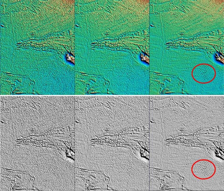
B01411                             SANDWELL AND SMITH: GLOBAL MARINE GRAVITY                                            B01411

         Figure 1. (top) Average of 10,000 Geosat radar waveforms (dotted) and a simplified model with five
         adjustable parameters: A, amplitude; to, arrival time; s, risetime; N, leading edge noise floor; k, trailing
         edge decay. The spacing of the gates is 3.12 ns or 468. mm. (bottom) Error in estimated arrival time
         versus error in estimated risetime for a synthetic experiment using realistic waveform data. The RMS
         error in arrival time is 28.4 for the unconstrained solution and 18.1 mm when the risetime was fixed.

least squares fit to each waveform, obtaining 2000 noisy          in an individual Geosat profile is about 24 km in the deep
estimates of each model parameter, and we examined the            ocean.
error distribution in these estimated parameters. The result        [14] To assess the reduction of noise due to retracking, we
of this simulation (Figure 1b) shows a severe correlation         compare sea surface slope along the GEOSAT GM profiles
between risetime and arrival time having a slope of 1. The        with the slope from our latest gravity model (version 18),
RMS scatter of the estimated arrival time about the true          presented in section 2.2. Since the model combines data from
arrival time is 28 mm. If we assume that the risetime varies      both ascending and descending tracks of Geosat, ERS-1,
smoothly along the satellite track because it reflects a
smoothly varying field of surface waves and we constrain
the risetime to the smoothed value, then the RMS scatter in
the estimated arrival time is 18 mm, or a 36% reduction in
RMS scatter (59% reduction in variance).
  [13] Improvements due to retracking of Geosat are char-
acterized in terms of both spatial resolution and noise level.
The spatial resolution is estimated by analyzing pairs of sea
surface height profiles from nearly collinear tracks and
performing a cross-spectral analysis of the height profile
pairs, assuming each is a realization of a random process
with coherent signal and incoherent noise [Bendat and
Piersol, 1986], as shown in Figure 2. The power spectra
of both signal and noise in sea surface height are shown,
before and after retracking. The noise power is cut nearly
50%, resulting in an improvement in spatial resolution of
nearly 5 km from 29 km to 24 km. These improvements               Figure 2. Power spectrum of sea surface height before
result in a noticeable sharpening of seafloor tectonic signals,   (gray) and after (black) retracking. Noise spectra are dashed
as well as a reduction in false sea surface height variability    while signal spectra are solid. Retracking cuts noise power
associated with increased SWH variability (e.g., in the           by 50% at mesoscale and shorter wavelengths. The spatial
Southern Ocean). The crossover point between signal and           resolution is also increased, since the signal power remains
noise also indicates that the shortest wavelength resolvable      above the noise power to shorter wavelengths.

                                                             3 of 18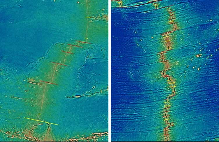
B01411 SANDWELL AND SMITH: GLOBAL MARINE GRAVITY B01411
and Topex, the comparison between model slopes and 1997] but with the following improvements. The grid cell
Geosat track slopes is not entirely circular thinking, and it size was reduced from 2 min to 1 min in an effort to retain
illustrates clearly the improvements due to retracking. higher spatial resolution. The latitude range was extended
Figure 3 shows the RMS difference between along-track from ±72° to ±80.7° to recover more gravity information in
slope from Geosat GM and the corresponding slope from the polar regions. This results in a grid of 2-byte integers
north and east vertical deflection grid products averaged at with 21,600 columns and 17,280 rows. Our model uses a
2 min resolution. The difference profiles are low-pass ‘‘remove-restore’’ procedure to blend short-wavelength de-
filtered with a Gaussian filter having a 0.5 gain at wave- tail from satellite altimetry with the large-scale anomalies of
lengths of 18 km (Figure 3, top and middle) and 80 km geopotential models; in 1997 we used the EGM96 model
(Figure 3, bottom). The RMS of the differences, averaged in (complete to degree 360, or 110 km wavelength), while we
0.25° cells, is displayed in Figure 3. The upper RMS now use the EGM2008 geoid height model complete to
difference map uses the original Geosat GM product tracked degree and order 2160 including the matching EGM2008
by the onboard a-b tracker [Lillibridge and Cheney, 1997] mean dynamic ocean topography (MDOT) model. In the
sampled at 5 Hz along track. The overall RMS difference is final iteration we also high-pass filter the residual slopes
4.4 mrad. The map shows three categories/areas where the (0.5 gain at 180 km wavelength) to further reduce the
RMS differences exceed the background value (2 mrad). influence of unmodeled dynamic ocean topography or tides.
First, there are latitudinal bands of high noise especially The short-wavelength detail is obtained by gridding the
between 30° and 60° south latitude. This noise is primarily residual sea surface slopes along altimeter tracks. In our
due to ranging from a surface that is roughened by high new model we use more data than in 1997, including
waves due to storms and high wind. The second type of retracked data, and we combine the data in a new way,
high noise area is associated with areas of very high sea using biharmonic splines with a tension parameter of 0.25
surface slope near large seamounts, fracture zones, and as described by Wessel and Bercovici [1998].
spreading ridges. This noise is primarily due to the 1.7 km [17] There are two major tasks in our data modeling
phase shift of the onboard tracker which causes a misalign- process. The first task is to build a seamless model of the
ment of the sharp feature with the feature recovered in the global marine geoid slope, that is, the north and east
profile. The third type of noise is due to mesoscale varia- components of the deflection of the vertical, by incorporat-
tions in sea surface slope associated with eddies and ing all available altimeter data and removing the sea surface
meandering currents [Cheney et al., 1983]. slope component due to dynamic ocean signals such as
[15] Figure 3 (middle) shows the same comparison but tides, mesoscale currents, and their eddies. The second task
after retracking the Geosat GM waveforms. The overall is to take the geoid slopes obtained in task one and convert
RMS difference is reduced to 3.2 mrad which corresponds to them to gravity anomalies. Only in this second task do we
a 27% improvement in RMS (47% in variance). Note the employ a gravity field model, such as EGM96 or
noise due to the rough ocean surface is dramatically EGM2008. Our data modeling process produces models
reduced. Also differences associated with very high sea of geoid slope as well as gravity anomalies.
surface slope are mostly gone. These two reductions in [18] To begin the modeling of geoid slope, we remove the
noise are due to the retracking which reduces the sensitivity UT CSR 4.0 tide model [Bettadpur and Eanes, 1994] from
of the range due to ocean waves and also corrects the phase each altimeter profile’s sequence of height samples taken at
shift from the onboard tracker. Unfortunately, the ‘‘noise’’ the highest available data rate (10 Hz or 20 Hz, depending
due to mesoscale ocean variability remains. Indeed addi- on the satellite). The data are low-pass filtered with a cut
tional smoothing of the slope differences along track that begins at 26.8 km wavelength, has 0.5 gain at 14.6 km,
(Figure 3, bottom) further highlights the spatial variations and zeros at 10 km; this filter was designed in Matlab using
in slope variability and the association of areas of higher the Parks-McClellan algorithm. After this filter is applied
variability with deeper [Sandwell and Zhang, 1989] and the data can be downsampled to a 5 Hz sampling rate,
smoother [Gille et al., 2000] seafloor. Assuming that the which corresponds to an along-track spacing of 1.4 km.
RMS differences at wavelengths longer than 80 km are all Because the data in the stacks of GEOSAT ERM and TOPEX
due to ocean processes, one can estimate the slope error due were acquired with the onboard tracker, we applied an
to ranging noise as 2.8 mrad, which corresponds to 2.8 mGal. additional filter to these stacked data to undo (as much as
Below we will confirm this noise level through a compar- possible) the along-track phase shift and group delay asso-
ison with shipboard gravity measurements. ciated with the onboard tracker as described by W. H. F.
Smith and D. T. Sandwell (manuscript in preparation,
2.2. Geoid Slope and Gravity Anomaly Model 2009). After this initial filtering we have sea surface height
Construction data from all seven data sources in the same form, with the
[16] The marine gravity field model was constructed as same sampling rate and without phase shifts.
described in our previous publication [Sandwell and Smith,
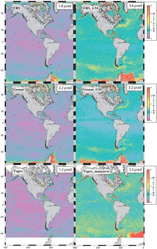
Figure 3. (top) RMS deviation of along-track slopes from the Geosat GM data from onboard tracking with respect to
slopes derived from our best estimate of the gravity field (this paper). The global RMS variation is 4.4 mrad. (middle) RMS
deviation of along-track slopes from retracked Geosat GM data with respect to slopes derived from our best estimate of the
gravity field has a global RMS of 3.19 mrad or a 27% improvement. (bottom) Along-track slope differences (retracked) but
low-pass filtered at 80 km wavelength. This RMS deviation of 1.56 mrad is mostly real signal due to mesoscale variations in
ocean surface slope.
4 of 18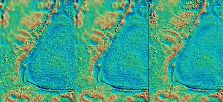
B01411   SANDWELL AND SMITH: GLOBAL MARINE GRAVITY   B01411

                         Figure 3

                           5 of 18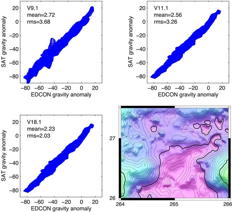
B01411                                     SANDWELL AND SMITH: GLOBAL MARINE GRAVITY                                                   B01411

Table 1. Summary of Slope Data and A Priori Uncertainties Used                  to assume that the mean anomaly is small over a patch area
for Gravity Model Constructiona                                                 for calculating the best spline fit to the seven altimeter data
                                             Number of                          sources, as discussed below.
                                            Observations         Uncertainty      [22] Our models ‘‘feel’’ the influence of the spherical
                                               (106)               (mrad)       harmonic model most strongly near shorelines. The altim-
GEOSAT GM                                        125                8.2         eter data cannot furnish information about the geoid slope
ERS-1 GM                                         111                9.7
ERS-1 ERM (35-day repeat)                        9.2                4.7
                                                                                over land, and our residual slopes taper smoothly to zero in
GEOSAT ERM (17 day repeat)                       4.8                7.5         land areas. The Laplace boundary value problem is solved
TOPEX ERM (10 day repeat)                        2.8                4.5         as a convolution, so that the gravity anomaly at a point
TOPEX (maneuver)                                 20                 12.6        depends on deflections in a region around that point. Our
ERS GM - polar (threshold retrack)               9.6                30.         prior models used EGM96, which furnished information to
   a
    Note that these 5 Hz data have minimal along-track filtering (0.5 gain at   harmonic degree 360, or about 100 km wavelength, and so
9 km wavelength), whereas the low-pass filter applied for the noise analysis
shown in Figure 3 was 18 km.
                                                                                our solutions began to degrade as one moved closer to shore
                                                                                than 50 km. Our latest solutions use EGM2008, complete to
                                                                                degree 2160, or about 19 km wavelength, so our solutions
                                                                                should feel the lack of land data only about 10 km from
                                                                                shore.
  [19] The along-track sea surface slope of each profile is                       [23] Our model development actually involved two iter-
then computed and compared to our prior models of geoid                         ations and interactions with the group developing EGM2008
slope, for two reasons. First, the prior model furnishes a                      [Pavlis et al., 2008]. First, we constructed a gravity model
sanity check that allows us to detect outliers that produce                     V16.1 combining all our retracked altimetry and the seven
spurious slopes. Our edit threshold was set at three times                      sources of data, but using the EGM96, complete to degree
the standard deviation given in Table 1. Second, we filter                      and order 360, as a reference field. The largest source of
(0.5 gain at 180 km wavelength) the differences in slope                        error in our V16.1 gravity grids is within 50 km of shore
between the profile and the model to remove long-wavelength                     [Maia, 2006] because of the zeros on land in the residual
profile slope components due to unmodeled tides, currents,                      deflection data. We hoped the group developing EGM2008
and eddies. After these steps the remaining sea surface slope                   might use our deflections at sea; however, they preferred to
data are presumed to measure geoid slope, that is, deflection                   use the gravity anomalies from our V16.1 field. These ocean
of the vertical. Verification that this is the case comes after                 data were combined with land and shipboard gravity data as
the geoid slopes have been converted to gravity anomalies,                      well as longer-wavelength (>400 km) satellite gravity
when we can compare these gravity anomalies to those                            information to construct a new global reference field com-
measured by ships carrying gravimeters.                                         plete to degree and order 2160 called EGM2007b. The
  [20] The conversion of vertical deflections to gravity                        EGM team provided us with this new model, which we then
anomalies is a boundary-value problem for Laplace’s equa-                       used in our remove/restore procedure to construct a second
tion. The most accurate computations use spherical harmon-                      marine gravity model called V17.1. Because this model
ics at long wavelengths, supplemented by Fourier                                included more complete land gravity information during the
transforms on data conformally projected onto a flat plane                      slope-to-gravity conversion, the errors in nearshore areas
for short wavelengths. We follow a standard practice in                         were presumably reduced. To reiterate, our north and east
geodesy known as a ‘‘remove-restore procedure’’: a spher-                       deflection grids from version 16.1 and 17.1 are identical;
ical harmonic model such as EGM96 or EGM2008 fur-                               only the gravity models are different and the differences are
nishes long-wavelength deflections and gravity anomalies,                       small except near shorelines. The EGM team then used the
the deflections are removed from our data, the residual                         V17.1 gravity model in the final construction of EGM2008.
deflections are converted to residual gravity anomalies by                      Close to the shorelines, the land data available in EGM2008
Fourier transform, the residual anomalies are then added to                     improves the accuracy of our nearshore marine gravity
the spherical harmonic model anomalies to obtain the total                      anomalies.
anomaly field.                                                                    [24] An additional improvement in our version 18.1 over
  [21] It is important to understand that use of this proce-                    our version 17.1 comes from the EGM2008 mean dynamic
dure does not imply that our model exactly matches the                          topography model. For version 18.1 we removed the slope
spherical harmonic model at all wavelengths contained in                        of this model from our deflections. The slope of the mean
the spherical harmonic model. In principle, if our data                         dynamic ocean topography is negligible except where
disagree with the EGM model at any wavelength, then                             western boundary currents that produce large ocean surface
there will be power in our residual at that wavelength, and                     slopes (1 – 10 mrad) remain spatially fixed over time.
so our data may be used to improve the model at all                               [25] All of these fields (V16 – 18) use the same along-
wavelengths. In practice, however, the Fourier transform                        track altimeter slopes derived from seven data sources as
calculation must be confined to a limited range of latitudes                    described in Table 1 in their order of importance. Almost all
where the conformal projection has a limited range of                           of the gravity information comes from the retracked profiles
scales, so that the flat-earth approximation is valid, and this                 of the GEOSAT GM and ERS-1 GM. Nevertheless the other
limits the longest wavelengths (650 km) at which the                           data sets provide targeted new information. For example,
altimeter data may influence the model. Common practice                         the 501 tracks of the ERS-1 exact repeat mission (ERM)
in geodesy uses ‘‘least squares collocation’’ to model the                      provide significant new information at high latitudes where
residual anomalies and usually assumes that the mean value                      the tracks converge and the stacking of multiple cycles
of the residual anomaly will be zero. We find it convenient                     provides coverage in ice-free times. The TOPEX ERM data

                                                                           6 of 18
B01411                                 SANDWELL AND SMITH: GLOBAL MARINE GRAVITY                                                 B01411

provide minimal new information along 127 tracks. How-             The coefficients cj represent the strength of each point load
ever, during September of 2002 the TOPEX track was                 applied to the thin elastic plate. They are found by solving
maneuvered to bisect the original 127 tracks. These data,          the following linear system of equations.
which we call TOPEX maneuver, provide some new infor-
mation although we show below that the noise level of the                                   X
                                                                                            N
data is significantly higher than GEOSAT GM data. Finally                  si ¼ ðrw nÞi ¼          cj rf xi  xj ni       i ¼ 1; N   ð4Þ
                                                                                             j¼1
we have included some ERS GM data at high latitudes (>65°)
that were retracked using a simple threshold retracker. This
retracker is able to provide sensible range estimates in ice       One issue that must be addressed is the possibility of having
covered areas where the three-parameter ocean waveform             two data constraints in exactly (or nearly) the same location.
retracker fails. However, these data are extremely noisy and       This causes the linear system to be exactly singular (or
are given very high uncertainty in the least squares estima-       numerically unstable) [Sandwell, 1987]. Our satellite
tion process (Table 1).                                            altimeter data commonly have many crossing profiles so it
  [26] Prior to filtering, the along-track slope profiles were     is possible to have two or even six slope constraints at
compared with a previous model to detect and edit outliers;        nearly the same location. The solution to this problem is to
the edit threshold was set at 3 times the standard deviation       reduce the number of Greens functions (knots) by making
given in Table 1. Along-track slopes from the EGM2008              sure they are not more closely spaced than some prescribed
geoid plus MDOT model [Pavlis et al., 2008] were removed           distance. That minimum distance should be about 1/4 of
and the residuals were gridded using a biharmonic spline           the shortest wavelength that one hopes to resolve. When
approach discussed next.                                           the number of knot locations is less than the number of
  [27] Consider N estimates of slope s(xi) with direction ni       constraints then the linear system is overdetermined and the
each having uncertainty si. We wish to find the ‘‘smooth-          surface will not exactly match the slope constraints. Since
est’’ surface w(x) that is consistent with this set of data such   we only wish to match the slopes to within the expected
that si = (rw . n)i. As in many previous publications we           uncertainty of each data type, each equation (4) should be
develop a smooth model using a thin elastic plate that is          divided by the slope uncertainty to provide the optimal
subjected to vertical point loads [Briggs, 1974; Smith and         solution using a singular value decomposition algorithm. In
Wessel, 1990]. The loads are located at the locations of the       our case we are not interested in the absolute height of the
data constraints (knots) and their amplitudes are adjusted to      surface but just the local slope so our final result is the
match the observed slopes [Sandwell, 1987]. To suppress            gradient of the surface.
overshooting oscillations of the plate, tension can be applied
to its perimeter. Wessel and Bercovici [1998] solved this                                      X
                                                                                               N
                                                                                     rwðxÞ ¼             cj rf x  xj                ð5Þ
problem by first determining the Greens function for the                                           j¼1
deflection of a thin elastic plate in tension. The differential
equation is
                                                                   While this interpolation theory is elegant and very flexible,
                                                                   it is difficult to apply to the altimeter interpolation problem
                  a2 r4 fðxÞ  r2 fðxÞ ¼ dðxÞ               ð1Þ    because there are over 200 million observations to grid
                                                                   (Table 1). Consider gridding just 1000 slopes, the matrix of
where a is a length scale factor that controls the importance      the linear system in equation (4) could have 106 elements if
of the tension. High a results in biharmonic spline                all the knot points were retained. In practice we make the
interpolation which minimizes the strain energy in the plate       following compromises in order to grid this large and
but can produce undesirable oscillations between data              diverse set of data.
points [Sandwell, 1987]. Zero a results in harmonic                   [ 28 ] 1. The data are residuals with respect to the
interpolation, which results in a surface that has sharp local     EGM2008 model so we can assemble and grid the data in
perturbations at the locations of the data constraints. The        overlapping small areas. We expect the residuals will only
tension factor controls the shape of the interpolating surface.    have signal at wavelengths of less than 37 km. Therefore for
Through experimentation we find good-looking results               a 1-min Mercator grid at 70° latitude we use a subarea size
when the solution is about 0.33 of the way from the                of 64 64 points, which has a dimension of 40 km (120 km
biharmonic to the harmonic end-member. The Greens                  at the equator).
function for this differential operator is                            [29] 2. To avoid edge effects, the subareas have 100%
                                                               overlap and only the inner 32          32 interpolated cells are
                                 jxj         jxj                   retained. The global analysis has 675 539 subareas.
                 fðxÞ ¼ Ko             þ log                ð2Þ
                                  a           a                       [30] 3. The along-track slope data from each of the six
                                                                   possible slope directions (i.e., ascending and descending
where Ko is the modified Bessel function of the second kind        profiles from three satellite inclinations ERS, GEOSAT, and
and order zero. The smooth surface is a linear combination         TOPEX) and associated uncertainties are binned onto the
of these Greens functions each centered at the location of         regularly spaced 1 min Mercator grid, and only the median
the data constraint.                                               slope of each type is retained for fitting. At midlatitudes there
                                                                   are typically 2000– 3000 slope constraints/uncertainties per
                             X
                             N                                   subarea and typically 800 unique knot points. The original
                    wðxÞ ¼         cj f x  xj              ð3Þ    distribution of knot points matches the satellite tracks so the
                             j¼1
                                                                   spacing at the equator can be as small as 1.8 km. We further

                                                              7 of 18
B01411 SANDWELL AND SMITH: GLOBAL MARINE GRAVITY B01411
Table 2. RMS Altimeter Noise From A Posteriori Comparison With V18 Gravity Modela
GEOSAT ERS-1 TOPEX
ERM GM GM ERM
GM GM Onboard Retrack Retrack ERM Maneuver Onboard
Tracker Onboard Retrack Stack Ocean Ice Stack Onboard Stack
l > 18 km a 4.45 3.21 2.18 3.57 8.62 1.75 3.34 1.17
d 4.36 3.17 2.21 3.55 8.92 1.76 3.33 1.19
l > 80 km a 1.88 1.56 1.15 1.63 2.98 1.02 1.50 0.73
d 1.85 1.55 1.15 1.62 3.16 1.02 1.50 0.74
a
Altimeter noise is measured in mrad. Values in bold represent ascending (a) and descending (d) data used in gravity model construction.
reduce the knot spacing to a minimum of 3 min (5.4 km) tracker) were stacked to form a single GEOSAT ERM
which seems to be sufficient to capture all the residual profile. The rms deviation is 2.2 mrad for wavelengths
signal for wavelengths >14 km. Since gridding is performed greater than 18 km and 1.2 mrad for wavelengths greater
in subareas, the computation time is inversely proportional than 80 km. The nonstacked GEOSAT GM data have higher
to the number of CPUs available. This analysis takes about RMS difference of 3.2 and 1.6 mrad, respectively. The main
a day of computer time when four processors are used. The features that can be summarized from this analysis are that
results of the computations are grids of residual east and the retracked GM data have an rms noise level of between
north vertical deflection that are converted to gravity 3.2 and 3.6 mrad for wavelengths greater than 18 km. The
anomalies and vertical gravity gradient as described in our stacked ERM profiles all have a lower noise level depend-
previous publication [Sandwell and Smith, 1997]. All grids ing approximately on the number of repeat cycles stacked.
are finally low-pass filtered using a filter with a 0.5 gain at The noise floor of about 1 mrad is due to a combination of
16 km, which is close to the cutoff wavelength of the 14.6 km errors such as summarized in Table 3. These estimates of
low-pass filter that was applied to the profiles. The combi- error are maximum values based on independent analyses
nation of the two filters has a cutoff wavelength of about and, in general, we find the measured noise for wavelengths
20 km which provides good looking results that also have greater than 80 km to be less than these estimates.
low RMS misfit to ground truth gravity anomalies collected [33] The maps of rms difference shown in Figure 4
by ships. One practical limitation of the current set of (western hemisphere only) reveal the spatial variations in
altimeter data is that a typical track spacing at the equator the altimeter noise. The differences from the ERM profiles
is 5 km so one cannot expect to recover wavelengths much (maps in left column) are generally less than 1 mrad. Higher
shorter than 20 km. rms difference occurs in areas of steep geoid gradient
perhaps reflecting the fact that these data were assembled
3. Results from onboard tracked profiles so the inverse alpha-beta
tracker described above does not completely undo the
3.1. Gravity Accuracy
adverse effects of this causal filter. As expected the ERM
[31] The resulting vertical deflection and gravity anomaly profiles do not show high RMS differences in the areas of
grids are evaluated using two techniques. First, we examine the western boundary currents because both the model and
the rms misfit between the model and the along-track slopes stacked profile represent the long-term average slope across
from each of the seven data types. This analysis is good for these features. The rms differences of the GM profiles
examining the relative contributions of each of the data (maps in right column) are generally higher and, as
types as well as to examine spatial variations in rms misfit. expected, show the time variable effects of the western
The second analysis compares the model gravity anomalies boundary currents. One step in the slope profile preparation
to gravity anomalies collected by ships. This comparison briefly mentioned above is that, prior to regridding, the
provides a more independent assessment of data accuracy residual slopes were high-pass filtered using a filter with a
and resolution but is limited to a few small areas where 0.5 gain at 180 km wavelength. This filter was designed to
high-quality shipboard data are available. Indeed, Maia remove the time-varying slopes from the GM profiles
[2006] has performed a blind test of an earlier version of mainly associated with mesoscale eddies. All the rms
this gravity grid (V16.1 EGM96 was used as EGM2008 was difference maps show large differences in areas of seasonal
not available) and we present a summary of those findings and especially permanent ice cover. These large differences
below. are due to a combination of errors in the model and the
[32] The profile versus model evaluations are provided in profiles. The gravity anomalies in these areas will also be
Table 2 and Figure 4. Each of the three altimeters has data noisy. A more careful retracking of the data in the ice-
collected in the exact repeat mission (ERM) configuration covered areas can provide significant improvements in
as well as the nonrepeat geodetic mission (GM) configura- gravity anomaly accuracy [Laxon and McAdoo, 1994;
tion. For example, 66 repeat cycles of GEOSAT (onboard McAdoo and Laxon, 1997].
Figure 4. RMS differences between the along-track slope from altimeter profiles and the new gravity model averaged
from 1 min to 2 min resolution. Differences were further filtered with a Gaussian filter having a 0.5 gain at 18 km. The
stacked profiles from the exact repeat missions (left column) have lower noise than the geodetic missions.
8 of 18B01411 SANDWELL AND SMITH: GLOBAL MARINE GRAVITY B01411
Figure 4
9 of 18B01411 SANDWELL AND SMITH: GLOBAL MARINE GRAVITY B01411
Table 3. Estimated Maximum Error in Sea Surface Slope relatively short wavelength and low amplitude in relation to
Slope the noise. There is a large mean difference between the ship
Signal or Error Source Length (km) Height (cm) (mrad) and altimeter-derived gravity that is probably due to an
Gravity signal 12 – 400 1 – 300 1 – 300 inaccurate gravity tie value in one of the ports [Wessel and
Orbit errorsa 8000 – 20,000 400 – 1000 900 20 100 3–6 20B01411 SANDWELL AND SMITH: GLOBAL MARINE GRAVITY B01411
Figure 5. (top) Shaded gravity anomaly for a large region in the Central Pacific Ocean centered at the
Galapagos Triple Junction (latitude 11° to 8°, longitude 255° to 270°). Colors saturate at ±60 mGal.
The visual noise level decreases as one moves from V9.1 (left) to V11.1 (center) to V18.1 (right). The
axis of the East Pacific Rise is well defined in V18.1 but more difficult to trace in V9.1 because of the
higher noise level. The red oval outlines a patch of small uncharted seamounts not apparent in V9.1.
(bottom) Vertical gravity gradient, or curvature of the geoid, for the same region.
Figure 6. Shaded gravity anomaly for a large region in the South Atlantic centered at the Falkland
Basin (latitude 57° to 27°, longitude 294° to 318°). Colors saturate at ±80 mGal. The visual noise
level decreases as one moves from V9.1 (left) to V11.1 (center) to V18.1 (right). Small-scale gravity
structure is visually apparent in V18.1 but hidden in the higher noise of V9.1. Note also the NW-trending
striped noise in V11.1 that is largely absent in V18.1. This noise is due to mesoscale ocean variability
which has been suppressed by the additional high-pass filter (180 km wavelength) used in V18.1.
11 of 18B01411 SANDWELL AND SMITH: GLOBAL MARINE GRAVITY B01411
Figure 7. Comparison between satellite-derived gravity models (thin lines) and a shipboard gravity
profile (points) across the Java Sea. (top) Gravity model version 9.1 does not use retracked altimeter data
and has an RMS misfit of 5.62 mGal. The mean difference of 25 mGal is due to a mean error commonly
found in shipboard gravity [Wessel and Watts, 1988]. (middle) Gravity model version 11.1 uses retracked
ERS-1 altimeter data but the Geosat data were not retracked; the RMS misfit is improved by nearly 1
to 4.75 mGal. (bottom) Gravity model version 18.1 is based on both retracked ERS-1 and Geosat
altimeter profiles and also used the biharmonic spline interpolation method. The RMS is improved further
to 3.03 mGal, which is a 46% reduction in rms.
gravity gradient used as shading on the new global bathym- tle upwellings [Lin and Phipps Morgan, 1992; Magde and
etry grid at 1 min resolution (Figure 10) helps to delineate Sparks, 1997; Parmentier and Phipps Morgan, 1990;
the first- and second-order segmentation of the mid-ocean Schouten et al., 1985], and minimum energy and damage
ridges [Macdonald et al., 1988]. A recent study of residual rheology configurations [Hieronymus, 2004; Lachenbruch,
mantle Bouguer anomaly by Gregg et al. [2007] using this 1973; Oldenburg and Brune, 1975]. Following the discov-
new V16.1 gravity grid reveals the spreading dependence of ery of transform faults more than 40 years ago, there is still
gravity anomalies along oceanic transform faults. Their no consensus on why they exist and why the ridge seg-
study combined with previous investigations on the varia- mentation varies with spreading rate. A leading hypothesis
tions in ridge-axis morphology with spreading rate is that transform faults and fracture zones provide a mech-
[Menard, 1967; Small, 1994], variations in abyssal hill anism for ridge-parallel shrinkage of the lithosphere. How-
morphology/seafloor roughness with spreading rate [Goff, ever, if this is correct then this mechanism should not be
1991; Goff et al., 2004; Small and Sandwell, 1992; Smith, effective on faster spreading ridges where the transform
1998], and the order of magnitude variations in seismic spacing is large. Perhaps other types of cracking and plate
moment release with spreading rate [Bird et al., 2002] bending occur along the fast spreading ridges [Gans et al.,
highlight the importance of spreading rate in lithospheric 2003; Sandwell and Fialko, 2004]. If the plates do not
strength and crustal structure. This is a first-order aspect of shrink in the ridge-parallel direction then large cracks may
plate tectonics that deserves a more comprehensive analysis. penetrate 30 km deep into the lithosphere as proposed by
[39] A more poorly understood phenomenon is the vari- Korenaga [2007]. Another possibility is that plates readily
ation in ridge segmentation with spreading rate [Abbott, contract in all three dimensions. In this case the lateral
1986; Sandwell, 1986]. A variety of models have been shrinkage will appear as significant perturbations to the
proposed [Kastens, 1987] for ridge segmentation including: global plate motion models [Kumar and Gordon, 2009].
thermal contraction joints [Collette, 1974; Sandwell, 1986], [40] We have begun a more careful analysis of on-ridge
thermal bending stresses [Turcotte, 1974], segmented man- and off-ridge segmentation to help resolve these fundamen-
12 of 18B01411 SANDWELL AND SMITH: GLOBAL MARINE GRAVITY B01411
Figure 8. At the bottom right is shown a gravity anomaly map (5 mGal contours) derived from dense
shipboard surveys and believed to have submilligal relative accuracy. Also shown are regression plots of
satellite gravity versus ship gravity with RMS differences of 3.68 mGal for V9.1, 3.26 mGal for version
11.1, and 2.03 mGal for version 18.1.
tal issues related to cooling of the oceanic lithosphere. spreading rate [Small and Sandwell, 1994]. Because the
Preliminary results are shown in Figures 11 and 12 where transitions occur at the same intermediate spreading rate, it
we have digitized the first- and second-order discontinuities is likely that a single lithospheric or mantle upwelling
in the global spreading ridge and display the segment mechanism controls both processes. A better understanding
lengths as a function of present-day full spreading rate. of ridge segmentation will require a more complete analysis
The ridges not showing a clear orthogonal pattern of ridges of both ridge axis and ridge flank data that is now available
and transforms at this resolution were not analyzed. These from our new gravity model.
include the Reykjanes ridge and the northwest end of the
Southwest Indian ridge and the area around the Easter and 4. Conclusions
Juan Fernandez microplates. These preliminary results show
a systematic increase in ridge segment length with spread- [41] Satellite altimetry has provided the most comprehen-
ing rate although the relationship is not linear. The gray sive images of the gravity field of the ocean basins with
curve is a Gaussian moving average of the data with a sigma accuracies and resolution approaching typical shipboard
of 20 mm/a. There a change in ridge segment length versus gravity data. While many satellite altimeter missions have
spreading rate that is in accordance with the abrupt change been flown over the past 3 decades, only 4% of these data
in axial valley topography and gravity anomaly with have nonrepeat orbital tracks that are necessary for gravity
Figure 9. The map shows gravity anomaly (V18.1, contour interval 10 mGal) of area offshore the east coast of North
America where the Gulf Stream follows the continental margin. Track of shipboard gravity profile collected in 1977 is
shown by red line. (top and middle) Ship gravity (dots) and satellite gravity (line). The satellite altimeter profiles measure
the total slope of the ocean surface, which has a large permanent component that introduces a 5 – 10 mGal error in the V16.1
gravity model. (bottom) Low-pass filtered residual in the satellite gravity are smaller in V18.1 (1.89 mGal) than in V16.1
(3.14 mGal) because of the improved ocean dynamic topography model available in the EGM2008 field used in V18.1.
13 of 18B01411 SANDWELL AND SMITH: GLOBAL MARINE GRAVITY B01411
field recovery. Our analysis uses three approaches to reduce Smith, 2005] and 18 months of Geosat/GM data (this study)
the error in the satellite-derived gravity anomalies to 2 – resulting in improvements in range precision of 40% and
3 mGal from 5 to 7 mGal. First, we have retracked the raw 27%, respectively. Second, we have used the recently
waveforms from 11 months of ERS-1 data [Sandwell and published EGM2008 global gravity model at 5 min resolu-
Figure 9
14 of 18B01411 SANDWELL AND SMITH: GLOBAL MARINE GRAVITY B01411
Table 4. RMS Values for the Differences Between the Marine and surface slopes to depart from geoid slopes by 3 – 6 mrad
the Satellite Free Air Anomalies for the V16 Modela along the western boundary currents and the Antarctic
Profile Unfiltered Data Filtered Data Circumpolar Current. Comparisons between shipboard
Profile 1 3.9 3.6 (10 km) gravity and the global gravity grid show errors ranging
Profile 2 5.4 3.0 (20 km) from 2.0 mGal in the Gulf of Mexico to 4.0 mGal in areas
Profile 3 4.0 2.6 (20 km) with rugged seafloor topography. The largest errors of up to
Profile 4 8.6 1.8 (10 km)
Profile 5 4.0 2.7 (10 km)
20 mGal occur on the crests of large seamounts [Marks and
a Smith, 2007]. The main limitation of the gravity model is
RMS is measured in mGal. The second column displays the RMS
values for unfiltered marine data. The third column displays the values for
spatial resolution which is controlled by the spatial filters
filtered data. The cutoff wavelength is shown in brackets. After Maia used in the along-track and 2-D analyses. Because gravity
[2006]. depends on the slope of the ocean surface, and the altimeter
measures the sea surface height, which has a nearly white
noise spectrum, reducing the size of the filters results in
unacceptably high noise levels. We have adopted a com-
tion [Pavlis et al., 2008] in the remove/restore method to promise filter that has a 0.5 gain at a wavelength of 15 km.
provide 5-min resolution gravity over the land and 1-min A new higher precision altimeter mission having a longer
resolution (8 km 1/2 wavelength) over the ocean with a duration could reduce the noise by perhaps 5 times [Raney
seamless land to ocean transition. Third we have used a et al., 2003]. Images of the new gravity model reveal small-
biharmonic spline interpolation method including tension scale structure not apparent in the previously published
[Wessel and Bercovici, 1998] to construct residual vertical models [e.g., Sandwell and Smith, 1997]. In particular the
deflection grids from seven types of inconsistent along-track segmentation of the global spreading ridges by orthogonal
slope measurements. ridges and transform faults further reveals the variations in
[42] Two approaches are used to evaluate the accuracy ridge axis morphology with spreading rate. As a first step
and resolution of the new gravity model. Differences we have digitized the ridge plate boundary and examined
between slope measured along satellite altimeter profiles the variations in ridge segment length with increasing
and the along-track slope projected from the vertical de- spreading rate. For rates less than about 60 mm/a the typical
flection grids show two main sources of residual error in the ridge segment is 50 –80 km long while it increases dramat-
nonrepeat profiles. At smaller length scales (B01411 SANDWELL AND SMITH: GLOBAL MARINE GRAVITY B01411
Figure 11. Present-day spreading rate from DeMets et al. [1994] with segments digitized from latest
grids.
Figure 12. (a) Preliminary version of ridge segment length versus spreading rate. Grey line is Gaussian
moving average (sigma 20 mm/a). For rates less than about 70 mm/a the typical ridge segment length
varies from 50 to 100 km. At higher rates there is a wider variation in segment length with some segments
1000 km long. Note that the Reykjanes ridge was not included and there is a lack of transform fault
segmentation around the Easter and Juan Fernandez microplates [Naar and Hey, 1989]. (b) Axial valley
relief and axial gravity amplitude versus full spreading rate from Small and Sandwell [1994].
16 of 18B01411 SANDWELL AND SMITH: GLOBAL MARINE GRAVITY B01411
[43] Acknowledgments. We thank the associate editor and reviewers Goff, J. A., W. H. F. Smith, and K. M. Marks (2004), The contributions of
for suggesting improvements to the manuscript. This work was partly abyssal hill morphology and noise to altimetric gravity fabric, Oceano-
supported by the National Science Foundation (OCE NAG5 – 13673) and graphy, 17(1), 24 – 37.
the Office of Naval Research (N00014-06-1-0140). The manuscript contents Gregg, P. C., J. Lin, M. D. Behn, and L. G. J. Montesi (2007), Spreading
are solely the opinions of the authors and do not constitute a statement of rate dependence of gravity anomalies along oceanic transform faults,
policy, decision, or position on behalf of NOAA or the U. S. Government. Nature, 448, 183 – 187, doi:10.1038/nature05962.
Haxby, W. F., and J. K. Weissel (1986), Evidence for small-scale mantle
References convection from Seasat altimeter data, J. Geophys. Res., 91(B3), 3507 –
3520, doi:10.1029/JB091iB03p03507.
Abbott, D. (1986), A statistical correlation between ridge crest offsets and Haxby, W. F., G. D. Karner, J. L. LaBrecque, and J. K. Weissel (1983),
spreading rate, J. Geophys. Res., 13, 157 – 160. Digital images of combined oceanic and continental data sets and their
Amarouche, L., P. Thibaut, O. Z. Zanife, J.-P. Dumont, P. Vincent, and use in tectonic studies, Eos Trans. AGU, 64(52), 995 – 1004.
N. Steunou (2004), Improving the Jason-1 ground retracking to better Hieronymus, C. F. (2004), Control on seafloor spreading geometries by
account for attitude effects, Mar. Geod., 27, 171 – 197, doi:10.1080/ stress- and strain-induced lithospheric weakening, Earth Planet. Sci.
01490410490465210. Lett., 222, 177 – 189, doi:10.1016/j.epsl.2004.02.022.
Andersen, O. B., and P. Knudsen (1998), Global marine gravity field from Hwang, C., and B. Parsons (1996), An optimal procedure for deriving
the ERS-1 and GEOSAT geodetic mission altimetry, J. Geophys. Res., marine gravity from multi-satellite altimetry, J. Geophys. Int., 125,
103, 8129 – 8137, doi:10.1029/97JC02198. 705 – 719, doi:10.1111/j.1365-246X.1996.tb06018.x.
Baudry, N., and S. Calmant (1991), 3-D Modelling of seamount topography Imel, D. A. (1994), Evaluation of the TOPEX/POSEIDON dual-frequency
from satellite altimetry, Geophys. Res. Lett., 18, 1143 – 1146, doi:10.1029/ ionospheric correction, J. Geophys. Res., 99, 24,895 – 24,906,
91GL01341. doi:10.1029/94JC01869.
Bendat, J. S., and A. G. Piersol (1986), Random Data Analysis and Mea- Jayne, S. R., L. C. St. Laurent, and S. T. Gille (2004), Connections between
surement Procedures, 2nd ed., 566 pp., John Wiley, New York. ocean bottom topography and the Earth’s Climate, Oceanography, 17(1),
Bettadpur, S. V., and R. J. Eanes (1994), Geographical representation of 65 – 74.
radial orbit perturbations due to ocean tides: Implications for satellite Jung, W. Y., and P. R. Vogt (1992), Predicting bathymetry from Geosat-
altimetry, J. Geophys. Res., 99, 24,883 – 24,898, doi:10.1029/94JC02080. ERM and shipborne profiles in the South Atlantic ocean, Tectonophysics,
Bird, P., Y. Y. Kagan, and D. D. Jackson (2002), Plate tectonics and earth- 210, 235 – 253, doi:10.1016/0040-1951(92)90324-Y.
quake potential of spreading ridges and oceanic transform faults, in Plate Kastens, K. K. (1987), A compendium of causes and effects of processes at
Boundary Zones, Geodyn. Ser., vol. 30, edited by S. Stein and J. T. transform faults and fracture zones, Rev. Geophys., 25(7), 1554 – 1562,
Freymueller, pp. 203 – 218, AGU, Washington, D.C. doi:10.1029/RG025i007p01554.
Briggs, I. C. (1974), Machine contouring using minimum curvature, Geo- Klees, R., R. Koop, P. Visser, and J. van den IJssel (2000), Efficient gravity
physics, 39, 39 – 48, doi:10.1190/1.1440410. field recovery from GOCE gravity gradient observations, J. Geod., 74(7 –
Brown, G. S. (1977), The average impulse response of a rough surface and 8), 561 – 571, doi:10.1007/s001900000118.
its application, IEEE Trans. Antennas Propag., 25(1), 67 – 74, Korenaga, J. (2007), Thermal cracking and deep hydration of oceanic litho-
doi:10.1109/TAP.1977.1141536. sphere: A key to generation of plate tectonics?, J. Geophys. Res., 112,
Brown, J., A. Colling, D. Park, J. Phillips, D. Rothery, and J. Wright (1998), B05408, doi:10.1029/2006JB004502.
The Ocean Basins: Their Structure and Evolution, 171 pp., Pergamon, Kumar, R. R., and R. G. Gordon (2009), Horizontal thermal contraction of
Oxford, U. K. oceanic lithosphere: The ultimate limit to the rigid plate approximation,
Cande, S. C., J. M. Stock, R. D. Mueller, and T. Ishihara (2000), Cenozoic J. Geophys. Res., 114, B01403, doi:10.1029/2007JB005473.
motion between East and West Antarctica, Nature, 404, 145 – 150, Kunze, E., and S. G. Llewellyn Smith (2004), The role of small-scale
doi:10.1038/35004501. topography in turbulent mixing of the global ocean, Oceanography,
Cazenave, A., P. Schaeffer, M. Berge, and C. Brossier (1996), High-resolu- 17(1), 55 – 64.
tion mean sea surface computed with altimeter data of ERS-1(Geodetic Lachenbruch, A. H. (1973), A simple mechanical model for oceanic spreading
Mission) and TOPEX-POSEIDON, Geophys. J. Int., 125(3), 696 – 704, centers, J. Geophys. Res., 78, 3395 – 3417, doi:10.1029/JB078i017p03395.
doi:10.1111/j.1365-246X.1996.tb06017.x. Lawver, L. A., L. M. Gahagan, and M. F. Coffin (1992), The development
Chelton, D. B., J. C. Reis, B. J. Haines, L. L. Fu, and P. S. Callahan (2001), of paleoseaways around Antarctica, in The Antarctic Paleoenvironment:
Satellite altimetry, in Satellite Altimetry and Earth Sciences, edited by A Perspective on Global Change, Geophys. Monogr. Ser., vol. 56, edited
L. L. Fu and A. Cazenave, pp. 1 – 131, Academic, San Diego, Calif. by J. P. Kennett and D. A. Warnke, pp. 7 – 30, AGU, Washington, D. C.
Cheney, R., J. Marsh, and B. Becklet (1983), Global mesoscale variability Laxon, S., and D. McAdoo (1994), Arctic Ocean gravity field derived from
from collinear tracks of SEASAT altimeter data, J. Geophys. Res., 88, ERS-1 satellite altimetry, Science, 265(5172), 621 – 624, doi:10.1126/
4343 – 4354, doi:10.1029/JC088iC07p04343. science.265.5172.621.
Collette, B. (1974), Thermal contraction joints in spreading seafloor as Lemoine, F. G., et al. (1998), The development of the joint NASA CSFC
origin of fracture zones, Nature, 251, 299 – 300, doi:10.1038/251299a0. and the national Imagery and Mapping Agency (NIMA) geopotential
DeMets, C., R. G. Gordon, D. F. Argus, and S. Stein (1994), Effect of model EGM96, 320 pp., NASA Goddard Space Flight Cent., Greenbelt,
recent revisions to the geomagnetic reversal timescale on estimates of Md.
current plate motions, Geophys. Res. Lett., 21, 2191 – 2194, doi:10.1029/ Le-Traon, P.-Y., and R. Morrow (2001), Ocean currents and eddies, in
94GL02118. Satellite Altimetry and Earth Sciences, edited by A. Cazenave and L.-L.
Dixon, T. H., M. Naraghi, M. K. McNutt, and S. M. Smith (1983), Bathy- Fu, pp. 175 – 215, Academic, San Diego, Calif.
metric prediction from Seasat altimeter data, J. Geophys. Res., 88, 1563 – Lillibridge, J., and R. Cheney (1997), The Geosat Altimeter JGM-3 GDRs
1571, doi:10.1029/JC088iC03p01563. [CD-ROM], NOAA, Silver Spring, Md.
Fairhead, J. D., C. M. Green, and M. E. Odegard (2001), Satellite-derived Lillibridge, J. L., W. H. F. Smith, R. Scharrroo, and D. T. Sandwell (2004),
gravity having an impact on marine exploration, Leading Edge, 20, 873 – The Geosat geodetic mission 20th anniversary data product, Eos Trans.
876. AGU, 85(47), Fall Meet. Suppl., Abstract SF43A – 0786.
Fu, L.-L., and A. Cazenave (2001), Satellite Altimetry and Earth Sciences: Lin, J., and J. Phipps Morgan (1992), The spreading rate dependence of
A Handbook of Techniques and Applications, 463 pp., Academic, San three-dimensional mid-ocean ridge gravity structure, Geophys. Res. Lett.,
Diego, Calif. 19, 13 – 16, doi:10.1029/91GL03041.
Fu, L.-L., and D. B. Chelton (2001), Large-scale ocean circulation, in Macdonald, K. C., P. J. Fox, L. J. Perram, M. F. Eisen, R. M. Haymon, S. P.
Satellite Altimetry and Earth Sciences, edited by A. Cazenave and L.-L. Miller, S. M. Carbotte, M. H. Cormier, and A. N. Shor (1988), A new
Fu, pp. 133 – 169, Academic, San Diego, Calif. view of the mid-ocean ridge from the behavior of ridge-axis discontinu-
Gans, K. D., D. S. Wilson, and K. C. Macdonald (2003), Pacific plate ities, Nature, 335(6187), 217 – 225, doi:10.1038/335217a0.
gravity lineaments: Extension or thermal contraction?, Geochem. Geo- Magde, L. S., and D. W. Sparks (1997), Three-dimensional mantle upwel-
phys. Geosyst., 4(9), 1074, doi:10.1029/2002GC000465. ling, melt generation, and melt migration beneath segment slow spread-
Gille, S. T., M. M. Yale, and D. T. Sandwell (2000), Global correlation ing ridge, J. Geophys. Res., 102, 20,571 – 20,583, doi:10.1029/
of mesoscale ocean variability with seafloor roughness from satellite 97JB01278.
altimetry, Geophys. Res. Lett., 27(9), 1251 – 1254, doi:10.1029/ Maia, M. (2006), Comparing the use of marine and satellite data for geo-
1999GL007003. dynamic studies, paper presented at 15 Years of Progress in Radar Alti-
Goff, J. A. (1991), A global and regional stochastic-analysis of near-ridge metry Symposium, Eur. Space Agency, Venice, Italy.
abyssal hill morphology, J. Geophys. Res., 96(B13), 21,713 – 21,737, Marks, K. M., and W. H. F. Smith (2007), Some remarks on resolving sea-
doi:10.1029/91JB02275. mounts in satellite gravity, Geophys. Res. Lett., 34, L03307, doi:10.1029/
2006GL028857.
17 of 18You can also read