Fractional Norms and Quasinorms Do Not Help to Overcome the Curse of Dimensionality - MDPI
←
→
Page content transcription
If your browser does not render page correctly, please read the page content below
entropy
Article
Fractional Norms and Quasinorms Do Not Help to
Overcome the Curse of Dimensionality
Evgeny M. Mirkes 1,2,∗ , Jeza Allohibi 1,3       and Alexander Gorban 1,2
 1   School of Mathematics and Actuarial Science, University of Leicester, Leicester LE1 7HR, UK;
     jhaa1@leicester.ac.uk (J.A.); a.n.gorban@leicester.ac.uk (A.G.)
 2   Laboratory of Advanced Methods for High-Dimensional Data Analysis, Lobachevsky State University,
     603105 Nizhny Novgorod, Russia
 3   Department of Mathematics, Taibah University, Janadah Bin Umayyah Road, Tayba,
     Medina 42353, Saudi Arabia
 *   Correspondence: em322@le.ac.uk

 Received: 4 August 2020; Accepted: 27 September 2020; Published: 30 September 2020

 Abstract: The curse of dimensionality causes the well-known and widely discussed problems for
 machine learning methods. There is a hypothesis that using the Manhattan distance and even
 fractional l p quasinorms (for p less than 1) can help to overcome the curse of dimensionality in
 classification problems. In this study, we systematically test this hypothesis. It is illustrated that
 fractional quasinorms have a greater relative contrast and coefficient of variation than the Euclidean
 norm l2 , but it is shown that this difference decays with increasing space dimension. It has been
 demonstrated that the concentration of distances shows qualitatively the same behaviour for all
 tested norms and quasinorms. It is shown that a greater relative contrast does not mean a better
 classification quality. It was revealed that for different databases the best (worst) performance was
 achieved under different norms (quasinorms). A systematic comparison shows that the difference in
 the performance of kNN classifiers for l p at p = 0.5, 1, and 2 is statistically insignificant. Analysis of
 curse and blessing of dimensionality requires careful definition of data dimensionality that rarely
 coincides with the number of attributes. We systematically examined several intrinsic dimensions of
 the data.

 Keywords: curse of dimensionality; blessing of dimensionality; kNN; metrics; high dimension;
 fractional norm

1. Introduction
     The term “curse of dimensionality” was introduced by Bellman [1] in 1957. Nowadays, this is a
general term for problems related to high dimensional data, for example, for Bayesian modelling [2], nearest
neighbour prediction [3] and search [4], neural networks [5,6], radial basis function networks [7–10] and
many others. Many authors have studied the “meaningfulness” of distance based classification [11–13],
clustering [12,14] and outlier detection [13,15] in high dimensions. These studies are related to the
concentration of distances, which means that in high dimensional space the distances between almost all
pairs of points of a random finite set have almost the same value (with high probability and for a wide class
of distributions).
      The term “blessing of dimensionality” was introduced by Kainen in 1997 [16]. The “blessing of
dimensionality” considers the same effect of concentration of distances from the different point of
view [17–19]. The concentration of distances was discovered in the foundation of statistical physics
and analysed further in the context of probability theory [20,21], functional analysis [22], and geometry
(reviewed by [23–25]). The blessing of dimensionality allows us to use some specific high dimensional

Entropy 2020, 22, 1105; doi:10.3390/e22101105                                  www.mdpi.com/journal/entropy
Entropy 2020, 22, 1105 2 of 30
properties to solve problems [26,27]. One such property is the linear separability of random points
from finite sets in high dimensions [24,28]. A review of probability in high dimension, concentration
of norm, and many other related phenomena is presented in [20].
The curse of dimensionality was firstly described 59 years ago [1] and the blessing of
dimensionality was revealed 23 years ago [16]. The importance of both these phenomena increases in
time. The big data revolution leads to an increase of the data dimensionality, and classical machine
learning theory becomes useless in the post-classical world where the data dimensionality often
exceeds the sample size (and it usually exceeds the logarithm of the sample size that makes many
classical estimates pointless) [26]. The curse and blessing of dimensionality are two sides of the same
coin. A curse can turn into a blessing and vice versa. For example, the recently found phenomenon of
stochastic separability in high dimensions [24,29] can be considered as a “blessing” [28] because it is
useful for fast non-iterative corrections of artificial intelligence systems. On the other hand, it can be
considered as a “curse” [30]: the possibility to create simple and efficient correctors opens, at the same
time, a vulnerability and provides tools for stealth attacks on the systems.
Since the “curse of dimensionality” and the “blessing of dimensionality” are related to the concept
of high dimensionality, six different approaches to evaluation of dimension of data were taken into
consideration. Beyond the usual dimension of vector space [31] (the number of atteributes), we considered
three dimensions determined by linear approximation of data by principal components [32,33] with the
choice of the number of principal components in accordance with the Kaiser rule [34,35], the broken stick
rule [36] and the condition number of the covariance matrix [28,37]. We also considered the recently
developed separability dimension [28,38] and the fractal dimension [39]. We demonstrated on many
popular benchmarks that intrinsic dimensions of data are usually far from the dimension of vector space.
Therefore, it is necessary to evaluate the intrinsic dimension of the data before considering any problem
as high- or low-dimensional.
The l p functional k x k p in a d dimensional vector space is defined as
!1/p
d
kxk p = ∑ | xi | p
. (1)
i =1
The Euclidean distance is l2 and the Manhattan distance is l1 . It is the norm for p ≥ 1 and the
quasinorm for 0 < p < 1 due to violation of the triangle inequality [40]. We consider only the case
with p > 0. It is well known that for p < q we have k x k p ≥ k x kq , ∀ x.
Measuring of dissimilarity and errors using subquadratic functionals reduces the influence of
outliers and can help to construct more robust data analysis methods [14,41,42]. The use of these
functionals for struggling with the curse of dimensionality was proposed in several works [14,42–46].
In particular, Aggarwal et al. [14] suggested that “fractional distance metrics can significantly improve
the effectiveness of standard clustering algorithms”. Francois, Wertz, and Verleysen studied Relative
Contrast (RC) and Coefficient of Variation (CV) (called by them ‘relative variance’) of distances between
datapoints in different l p norms [42]. They found that “the ‘optimal’ value of p is highly application
dependent”. For different examples, the optimal p was equal to 1, 1/2, or 1/8 [42]. Dik et al. [43]
found that for fuzzy c-means usage of l p -quasinorms with 0 < p < 0.5 “improves results when
compared to p ≥ 0.5 or the usual distances, especially when there are outliers.” The purity of clusters
was used for comparison. Jayaram and Klawonn [44] studied RC and CV for quasinorms without
triangle inequality and for metrics unbounded on the unite cube. In particular, they found that
indicators of concentration of the norm are better for lower p and, moreover, that unbounded distance
functions whose expectations do not exist behave better than norms or quasinorms. France [45]
compared effectiveness of several different norms for clustering. They found that the normalised
metrics proposed in [46] give a better results and recommended to use the normalised l1 metrics for
nearest neighbours recovery.Entropy 2020, 22, 1105 3 of 30
In 2001, C.C. Aggarwal and co-authors [14] briefly described the effect of using fractional quasinorms
for high-dimensional problems. They demonstrated that using of l p (p ≤ 1) can compensate the
concentration of distances. This idea was used further in many works [13,47,48]. One of the main
problems of using the quasinorm l p for p < 1 is time of calculation of minimal distances and solution of
optimization problems with l p functional (which is even non-convex for p < 1). Several methods have
been developed to speed up the calculations [47,49].
The main recommendation of [14] was the use of Manhattan distance instead of Euclidean
one [50–52]. The main reason for this is that a smaller p is expected to give better results but for p < 1
the functional l p is not a norm, but a non-convex quasinorm. All methods and algorithms that assume
triangle inequality [51,53,54] cannot use such a quasinorm.
A comparison of different l p functionals for data mining problems is needed. In light of the
published preliminary results, for example, [14,55,56], more testing is necessary to evaluate the
performance of data mining algorithms based on these l p norms and quasinorms.
In our study, we perform systematic testing. In general, we demonstrated that the concentration
of distances for l p functionals was less for smaller p. Nevertheless, for all p, the dependences of
distance concentration indicators (RC p and CV p ) on dimension are qualitatively the same. Moreover,
the difference in distance concentration indicators for different p decreases with increasing dimension,
both for RC and CV.
The poor performance of k Nearest Neighbour (kNN) classifiers in high dimensions is used as a
standard example of the “curse of dimensionality” for a long time, from the early work [11] to the deep
modern analysis [57]. The kNN classifiers are very sensitive to used distance (or proximity) functions
and, therefore, they are of particular interest to our research.
We have systematically tested the hypothesis that measuring of dissimilarity by subquadratic
norms l p (1 ≤ p < 2) or even quasinorms (0 < p < 1) can help to overcome the curse of dimensionality
in classification problems. We have shown that these norms and quasinorms do not systematically and
significantly improve performance of kNN classifiers in high dimensions.
In addition to the main result, some simple technical findings will be demonstrated below that
can be useful when analyzing multivariate data. Two of them are related to the estimation of the
dimension of the data, and the other two consider the links between the use of different l p norms,
the concentration of distances and the accuracy of the kNN classifiers:
• The number of attributes for most of real life databases is far from any reasonable intrinsic
dimensionality of data;
• The popular estimations of intrinsic dimensionality based on principal components (Kaiser rule
and broken stick rule) are very sensitive to irrelevant attributes, while the estimations based
on the condition number of the reduced covariance matrix is much more stable as well as the
definitions based on separability properties or fractal dimension;
• Usage of l p functionals with small p does not prevent the concentration of distances;
• A lower value of a distance concentration indicator does not mean better accuracy of the
kNN classification.
Our paper is organized as follows. In Section 2, we present results of an empirical test
of distance concentration for relative contrast and coefficient of variation also known as relative
variance. Section 3 introduces the six used intrinsic dimensions. In Section 4, we describe the
approaches used for l p functionals comparison, the used databases and the classification quality
indicators. In Section 5, six intrinsic dimensions are compared for the benchmark datasets. In Section 6,
we compare performance of classifiers for different l p functionals. The ‘Discussion’ section provides
discussion and outlook. The ‘Conclusion’ section presents conclusions.
All software and databases used in this study are freely available online [58]. Some results of
this work were presented partially at IJCNN’2019 [59]: comparison of RC and CV (Section 2) and
comparison of l p functionals for 11NN classifier (part of Section 6).Entropy 2020, 22, 1105 4 of 30
2. Measure Concentration
Consider a database X with n data points X = { x1 , . . . , xn } and d real-valued attributes,
xi = ( xi1 , . . . , xid ). x without index is the query point: the point for which all distances were
calculated. We used for testing two types of databases: randomly generated databases with i.i.d.
components from the uniform distribution on the interval [0, 1] (this section) and real life databases
(Section 4). The l p functional for vector x is defined by (1). For comparability of results with [14],
in this study, we consider the set of norms and quasinorms used in [14] with one more quasinorm
(l0.01 ): l0.01 , l0.1 , l0.5 , l1 , l2 , l4 , l10 , l∞ .
Figure 1 shows the shapes of the unit level sets for all considered norms and quasinorms excluding
l0.01 and l0.1 . For two excluded quasinorms, the level sets are visually indistinguishable from the
central cross.
Figure 1. Unit level sets for l p functionals (“Unit spheres”).
Several different indicators were used to study the concentration of distances:
• Relative Contrast (RC) [11,14,42]
| maxi k xi − x k p − mini k xi − x k p |
RC p ( X, x ) = ; (2)
mini k xi − x k p
• Coefficient of Variations (CV) or relative variance [42,53,54]
q
var (k xi − x k p |)
CV p ( X, x ) = , (3)
mean(k xi − x k p )
where var (z) is the variance and mean(z) is the mean value of the random variable z;
• Hubness (popular nearest neighbours) [13].
In our study, we used RC and CV. Hubness [13] characterised distribution of the number
of k-occurrences of data points that is, the number of times the data point occurs among the k
nearest neighbours of all other data points. With dimensionality increase, the distribution this
k-occurrence becomes more skewed to the right, that indicates the emergence of hubs, i.e., popular
nearest neighbours which appear in many more kNN lists than other points. We did not use hubness
in our analysis because this change in the distribution of a special random variable, k-occurrence,
needs additional convention about interpretation. Comparison of distributions is not so illustrative as
comparison of real numbers.
Table 2 in paper [14] shows that the proportion of cases where RC1 > RC2 increases with
dimension. It can be easily shown that for special choice of X and x, all three relations between RC1 and
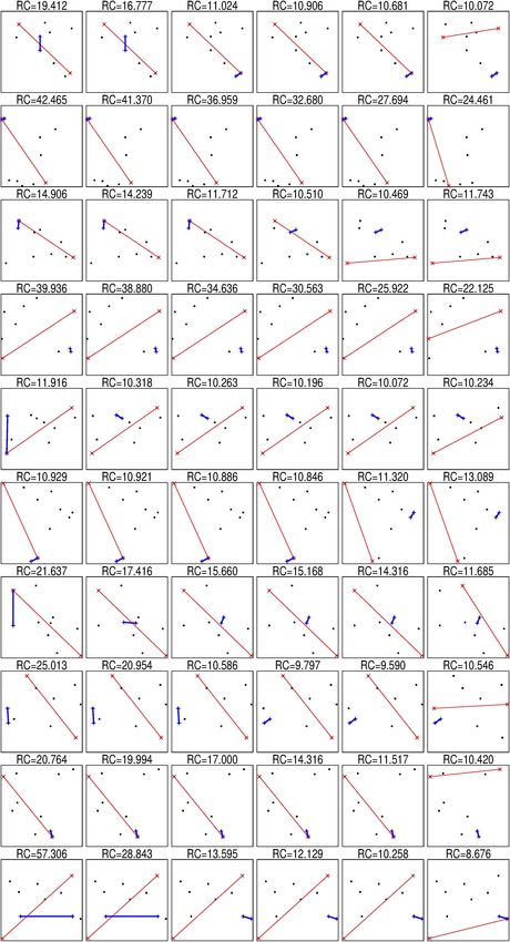
RC2 are possible : RC1 ( X, x ) > RC2 ( X, x ) (all lines in Figure 2, exclude row 6), RC1 ( X, x ) = RC2 ( X, x ),
or RC1 ( X, x ) < RC2 ( X, x ) (row 6 in Figure 2). To evaluate the probabilities of these three outcomes,
we performed the following experiment. We generated X dataset with k points and 100 coordinates.
Each coordinate of each point was uniformly randomly generated in the interval [0, 1]. For eachEntropy 2020, 22, 1105 5 of 30
dimension d = 1, 2, 3, 4, 10, 15, 20, 100, we created a d-dimensional dataset Xd by selecting the first d
coordinates of points in X. We calculated RC p as the mean value of RC for each point in Xd :
1 k
k i∑
RC p = RC p ( Xd \{ xi }, xi ), (4)
=1
where X \{ x } is the X database without the point x. We repeated this procedure 1000 times and
calculated the fraction of cases when RC1 > RC2 . The results of this experiment are presented in
Table 1. Table 1 shows that for k = 10 points our results are very similar to the results presented in
Table 2 in [14]. Increasing the number of points shows that even with a relatively small number of
points (k ≈ 20) for almost all databases RC1 > RC2 .
Table 1. Comparison of RC for l1 and l2 for different dimension of space (Dim) and different number
of points.
P (RC2 < RC1 ) for # of Points
Dim
10 [14] 10 20 100
1 0 0 0 0
2 0.850 0.850 0.960 1.00
3 0.887 0.930 0.996 1.00
4 0.913 0.973 0.996 1.00
10 0.956 0.994 1.00 1.00
15 0.961 1.000 1.00 1.00
20 0.971 0.999 1.00 1.00
100 0.982 1.000 1.00 1.00
We can see that appearance of a noticeable proportion of cases when RC2 > RC1 is caused by a
small sample size. For not so small samples, in most cases RC2 < RC1 . This is mainly because the
pairs of nearest (farthest) points can be different for different metrics. Several examples of such sets are
presented in Figure 2. Figure 2 shows that RC2 < RC∞ in rows 3, 5, 6, and 8 and RC1 < RC2 in row 6.
These results allow us to formulate the hypothesis that in general almost always RC p < RCq , ∀ p > q.
RC is widely used to study the properties of a finite set of points, but CV is more appropriate for point
distributions. We hypothesise that CV p < CVq , ∀ p > q.
To check these hypotheses, we performed the following experiment. We created a X database
with 10,000 points in 200 dimensional space. Each coordinate of each point was uniformly randomly
generated in the interval [0, 1]. We chose the set of dimensions d = 1, 2, 3, 4, 5, 10, 15, . . . , 195, 200 and
the set of l p functionals l0.01 , l0.1 , l0.5 , l1 , l2 , l4 , l10 , l∞ . For each dimension d, we prepared the Xd database
as the set of the first d coordinates of points in X database. For each Xd database and l p functional, we
calculate the set of all pairwise distances Ddp . Then, we estimated the following values:
q
max Ddp − min Ddp var ( Ddp )
RC p = , CV p = . (5)
min Ddp mean( Ddp )
The graphs RC p and CV p are presented in Figure 3. Figure 3 shows that our hypotheses hold.
We see that RC and CV as functions of dimension have qualitatively the same shape but in different
scales: RC in the logarithmic scale. The paper [14] states that the qualitatively different behaviour of
maxi k xi k p − maxi k xi k p was observed for different p. We found qualitatively the same behavior for
relative values (RC). The small quantitative difference RC p − RCq increases for d from 1 to about 10
and decreases with a further increase in dimension. This means that there could be some preference
for using lower values of p but the fractional metrics do not provide a panacea for the curse of
dimensionality. To analyse this hypothesis, we study the real live benchmarks in the Section 4.Entropy 2020, 22, 1105 6 of 30
Figure 2. Ten randomly generated sets of 10 points, thin red line connects the furthest points and bold
blue line connects closest points, columns (from left to right) corresponds to p = 0.01, 0.1, 0.5, 1, 2, ∞.Entropy 2020, 22, 1105 7 of 30
Figure 3. Changes of RC (left) and CV (right) with dimension for several metrics.
3. Dimension Estimation
To consider high dimensional data and the curse or blessing of dimensionality, it is necessary to
determine what dimensionality is. There are many different notions of data dimension. Evaluation of
dimensionality become very important with emergence of many “big data” databases. The number
of attributes is the dimension of the vector space [31] (hereinafter referred to as #Attr). For the data
mining tasks, the dimension of space is not as important as the data dimension and the intrinsic data
dimension is usually less than the dimension of space.
The concept of intrinsic, internal or effective data dimensionality is not well defined for the
obvious reason: the data sets are finite and, therefore, the direct application of topological definitions
of dimension gives zero. The most popular approach to determining the data dimensionality is
approximation of data sets by a continuous topological object. Perhaps, the first and at the same time
widely used definition of intrinsic dimension is the dimension of the linear manifold of “the best fit to
data” with sufficiently small deviations [32]. The simplest way to evaluate such dimension is Principal
Component Analysis (PCA) [32,33]. There is no single (unambiguous) method for determining the
number of informative (important, relevant, etc.) principal components [36,60,61]. The two widely
used methods are the Kaiser rule [34,35] (hereinafter referred to as PCA-K) and the broken stick
rule [36] (hereinafter referred to as PCA-BS).
Let us consider a X database with n data points X = x1 , . . . , xn and d real-valued attributes,
xi = ( xi1 , . . . , xid ). The empirical covariance matrix Σ( X ) is symmetric and non-negative definite.
The eigenvalues of the Σ( X ) matrix are non-negative real numbers. Denote these values as λ1 ≥ λ2 ≥
· · · ≥ λd . Principal components are defined using the eigenvectors of empirical covariance matrix
Σ( X ). If the ith eigenvector wi is defined then the ith principal coordinate of the datavector x is the
inner product ( x, wi ). The Fraction of Variance Explained (FVE) by ith principal component for the
dataset X is
λ
fi = d i .
∑ j =1 λ j
The Kaiser rule states that all principal components with FVE greater or equal to the average
FVE are informative. The average FVE is 1/d. Thus, the components with f i ≥ 1/d are considered
as informative ones and should be retained and the components with f i < 1/d should not. Another
popular version uses a twice lower threshold 0.5/d and retains more components.
The broken stick rule compares the set f i with the distribution of random intervals that appear if
we break the stick at d − 1 points randomly and independently sampled from the uniform distribution.
Consider a unit interval (stick) randomly broken into d fragments. Let us numerate these fragments in
descending order of their length: s1 ≥ s2 ≥ · · · ≥ sd . Expected length of i fragment is [36]Entropy 2020, 22, 1105 8 of 30
d
1 1
bi =
d ∑ j
. (6)
j =i
The broken stick rule states that the first k principal components are informative, where k is the
maximum number such that f i ≥ bi , ∀i ≤ k.
In many problems, the empirical covariance matrix degenerates or almost degenerates, that means
that the smallest eigenvalues are much smaller than the largest ones. Consider the projection of data
on the first k principal components: X̂ = XV, where the columns of the matrix V are the first k
eigenvectors of the matrix Σ( X ). Eigenvalues of the empirical covariance matrix of the reduced data
Σ( X̂ ) are λ1 , λ2 , . . . , λk . After the dimensionality reduction, the condition number (the ratio of the
lowest eigenvalue to the greatest) [62] of the reduced covariance matrix should not be too high in order
to avoid the multicollinearity problem. The relevant definition [28] of the intrinsic dimensionality
refers directly to the condition number of the matrix Σ( X̂ ): k is the number of informative principal
components if it is the smallest number such that
λ k +1 1
< , (7)
λ1 C
where C is specified condition number, for example, C = 10. This approach is further referred to
as PCA-CN. The PCA-CN intrinsic dimensionality is defined as the number of eigenvalues of the
covariance matrix exceeding a fixed percent of its largest eigenvalue [37].
The development of the idea of data approximation led to the appearance of principal
manifolds [63] and more sophisticated approximators, such as principal graphs and complexes [64,65].
These approaches provide tools for evaluating the intrinsic dimensionality of data and measuring the
data complexity [66]. Another approach uses complexes with vertices in data points: just connect the
points with distance less than ε for different ε and get an object of combinatorial topology, simplicial
complex [67]. All these methods use an object embedded in the data space. They are called Injective
Methods [68]. In addition, a family of Projective Methods was developed. These methods do not
construct a data approximator, but project the dataspace onto a space of lower dimension with
preservation of similarity or dissimilarity of objects. A brief review of modern injective and projective
methods can be found in [68].
Recent studies of curse/blessing dimensionality introduce a new method for evaluation intrinsic
dimension: separability analysis. A detailed description of this method can be found in [28,38]
(hereinafter referred to as SepD). For this study, we used an implementation of separability analysis
from [69]. The main concept of this approach is the α Fisher separability: point x of dataset X is α
Fisher separable from dataset X if
( x, y) ≤ α( x, x ), ∀y ∈ X, y 6= x, (8)
where ( x, y) is dot product of vectors x and y.
The last intrinsic dimension used in this study is the fractal dimension (hereinafter referred to as
FracD). It is also known as box-counting dimension or Minkowsk–Bouligand dimension. There are
many versions of box-counting algorithms and we used R implementation from the RDimtools
package [70]. The definition of FracD is
log( N (r ))
d f = lim ,
r →0 log(1/r )
where r is the size of the d-cubic box in the regular grid and N (r ) is the number of cells with data
points in this grid. Of course, formally this definition is controversial since the data set is finite andEntropy 2020, 22, 1105 9 of 30
there is no infinite sequence of discrete sets. In practice, the limit is substituted by the slope of the
linear regression for sufficiently small r but without intercept.
There are many approaches to non-linear evaluation of data dimensionality with various
non-linear data approximants: manifolds, graphs or cell complexes [63,65,66,68]. The technology
of neural network autoencoders is also efficient and very popular but its theoretical background is still
under discussion [71]. We did not include any other non-linear dimensionality reduction methods
in our study because there is a fundamental uncertainty: it is not known a priori when to stop the
reduction. Even for simple linear PCA, we have to consider and compare three stopping criteria,
from Kaiser rule to the condition number restriction. For non-linear model reduction algorithms
the choice of possible estimates and stopping criteria is much richer. The non-linear estimates of
the dimensionality of data may be much smaller than the linear ones. Nevertheless, for the real life
biomedical datasets, the difference between linear and non-linear dimensions is often not so large
(from 1 to 4), as it was demonstrated in [65].
4. Comparison of l p Functionals
In Section 2, we demonstrated that RC p is greater for smaller p. It was shown in [11] that greater
RC means ‘more meaningful’ task for kNN. We decided to compare different l p functions for kNN
classification. Classification has one additional advantage over regression and clustering problems:
the standard criteria of classification quality are classifier independent and and do not depend on the
dissimilarity measures used [72].
For this study, we selected three classification quality criteria: the Total Number of Neighbours of
the Same Class (TNNSC) (that is, the total number of the k nearest neighbors that belonged to the same
class as the target object over all the different target objects), accuracy (fraction of correctly recognised
cases), sum of sensitivity (fraction of correctly solved cases of positive class) and specificity (fraction of
correctly solved cases of negative class). TNNSC is not an obvious indicator of classification quality
and we use it for comparability of our results with [14]. kNN with 11 nearest neighbours was used
also for comparability with [14].
4.1. Databases for Comparison
We selected 25 databases from UCI Data repository [73]. To select the databases, we applied the
following criteria:
1. Data are not time-series.
2. Database is formed for the binary classification problem.
3. Database does not contain any missing values.
4. The number of attributes is less than the number of observations and is greater than 3.
5. All predictors are binary or numeric.
In total, 25 databases and 37 binary classification problems were selected (some databases contain
more than one classification problem). For simplicity, we refer to each task as a ‘database’. The list of
selected databases is presented in Table 2.
We do not set out to determine the best database preprocessing for each database. We just use
three preprocessing for each database:
• Empty preprocessing means usage data ‘as is’;
• Standardisation means shifting and scaling data to have a zero mean and unit variance;
• Min-max normalization refers to shifting and scaling data in the interval [0, 1].Entropy 2020, 22, 1105 10 of 30
Table 2. Databases selected for analysis.
Name Source #Attr. Cases PCA-K PCA-BS PCA-CN SepD FracD
Blood [74] 4 748 2 2 3 2.4 1.6
Banknote authentication [75] 4 1372 2 2 3 2.6 1.9
Cryotherapy [76–78] 6 90 3 0 6 4.1 2.5
Vertebral Column [79] 6 310 2 1 5 4.4 2.3
Immunotherapy [76,77,80] 7 90 3 0 7 5.1 3.2
HTRU2 [81–83] 8 17,898 2 2 4 3.06 2.4
ILPD (Indian Liver
Patient Dataset) [84] 10 579 4 0 7 4.3 2.1
Planning Relax [85] 10 182 4 0 6 6.09 3.6
MAGIC Gamma Telescope [86] 10 19,020 3 1 6 4.6 2.9
EEG Eye State [87] 14 14,980 4 4 5 2.1 1.2
Climate Model Simulation
Crashes [88] 18 540 10 0 18 16.8 21.7
Diabetic Retinopathy Debrecen [89,90] 19 1151 5 3 8 4.3 2.3
SPECT Heart [91] 22 267 7 3 12 4.9 11.5
Breast Cancer [92] 30 569 6 3 5 4.3 3.5
Ionosphere [93] 34 351 8 4 9 3.9 3.5
QSAR biodegradation [94,95] 41 1055 11 6 15 5.4 3.1
SPECTF Heart [91] 44 267 10 3 6 5.6 7
MiniBooNE particle
identification [96] 50 130,064 4 1 1 0.5 2.7
First-order theorem proving
(6 tasks) [97,98] 51 6118 13 7 9 3.4 2.04
Connectionist Bench (Sonar) [99] 60 208 13 6 11 6.1 5.5
Quality Assessment of
Digital Colposcopies (7 tasks) [100,101] 62 287 11 6 9 5.6 4.7
LFW [102] 128 13,233 51 55 57 13.8 19.3
Musk 1 [103] 166 476 23 9 7 4.1 4.4
Musk 2 [103] 166 6598 25 13 6 4.1 7.8
Madelon [104,105] 500 2600 224 0 362 436.3 13.5
Gisette [104,106] 5000 7000 1465 133 25 10.2 2.04
4.2. Approaches to Comparison
Our purpose is to compare l p functionals but not to create the best classifier for each problem.
Following [14], we use the 11NN classifier, and 3NN, 5NN and 7NN classifiers for more general result.
One of the reasons for choosing kNN is strong dependence of kNN on used metrics and, on the other
hand, the absence of any assumption about the data, excluding the principle: tell me your neighbours,
and I will tell you what you are. In our study, we consider kNN with l0.01 , l0.1 , l0.5 , l1 , l2 , l4 , l10 , l∞ as
different algorithms. We applied the following indicators to compare kNN classifiers (algorithms) for
listed l p functionals:
• The number of databases for which the algorithm is the best [107];
• The number of databases for which the algorithm is the worst [107];
• The number of databases for which the algorithm has performance that is statistically
insignificantly different from the best;
• The number of databases for which the algorithm has performance that is statistically
insignificantly different from the worst;Entropy 2020, 22, 1105 11 of 30
• The Friedman test [108,109] and post hoc Nemenyi test [110] which were specially developed to
compare multiple algorithms;
• The Wilcoxon signed rank test was used to compare three pairs of metrics.
We call the first four approaches frequency comparison. To avoid discrepancies, a description of
all used statistical tests is presented below.
4.2.1. Proportion Estimation
Since two criteria of classification quality – accuracy and TNNSC/(k × n), where n is the number
of cases in the database – are proportions, we can apply z-test for proportion estimations [111].
We want to compare two proportions with the same sample size, so we can use a simplified formula
for test statistics:
| p1 − p2 |
z= q , (9)
p1 + p2 p1 + p2
n 1 − 2
where p1 and p2 are two proportions for comparison. P-value of this test is the probability of observing
by chance the same or greater z if both samples are taken from the same population. P-value is
pz = Φ(−z), where Φ(z) is the standard cumulative normal distribution. There is a problem of
reasonable choice of significance level. The selected databases contain from 90 to 130,064 cases. Using
the same threshold for all databases is meaningless [112,113]. The required sample size n can be
estimated through the specified significance level of 1 − α, the statistical power 1 − β, the expected
effect size e, and the population variance s2 . For the normal distribution (since we use z-test) this
estimation is:
2 ( z 1− α + z 1− β )2 s 2
n= . (10)
e2
In this study, we assume that the significance level is equal to the statistical power α = β,
the expected effect size is 1% (1% difference in accuracy is large enough), and the population variance
can be estimated by the formula
n+ n+ n+ (n − n+ )
s2 = n 1− = , (11)
n n n
where n+ is the number of cases in the positive class. Based on this assumption, we can estimate a
reasonable level of significance as
r
e n
α=Φ . (12)
s 8
Usage of eight l p functionals means multiple testing. To avoid overdetection problem we
apply Bonferroni correction [114]. On the other hand, usage of too high a significance level is also
meaningless [112]. As a result, we select the significance level as
r
1 e n
α = max Φ , 0.00001 . (13)
28 s 8
The difference between two proportions (TNNSC or accuracy) is statistically significant if pz < α.
It must be emphasized that for TNNSC the number of cases is kn because we consider k neighbours
for each point.
4.2.2. Friedman Test and Post Hoc Nemenyi Test
One of the widely used statistical tests for comparing algorithms on many databases is the
Friedman test [108,109]. To apply this test, we firstly need to apply the tied ranking for the classification
quality score for one database: if several classifiers provide exactly the same quality score then the
rank of all such classifiers will be equal to the average value of the ranks for which they were tied [109].Entropy 2020, 22, 1105 12 of 30
We denote the number of used databases as N, the number of used classifiers as m and the rank of
classifier i for database j as r ji . The mean rank of classifier i is
N
1
Ri =
N ∑ r ji . (14)
j =1
Test statistics is
N 2 (m − 1) 4 ∑im=1 R2i − m(m + 1)2
χ2F = . (15)
4 ∑im=1 ∑ N 2
j=1 r ji − Nm ( m + 1)
2
Test statistics under null hypothesis that all classifiers have the same performance follows the χ2
distribution with m − 1 degrees of freedom. P-value of this test is the probability of observing by chance
the same or greater χ2F if all classifiers have the same performance. P-value is pχ = 1 − F (χ2F ; m − 1),
where F (χ; d f ) is the cumulative χ2 distribution with d f degrees of freedom. Since we only have 37
databases, we decide to use the 95% significance level.
If the Friedman test shows enough evidence to reject the null hypothesis, then we can conclude that
not all classifiers have the same performance. To identify pairs of classifiers with significantly different
performances, we applied the post hoc Nemenyi test [110]. Test statistics for comparing of classifiers i
and j is | Ri − R j |. To identify pairs with statistically significant differences the critical distance
r
m ( m + 1)
CD = qαm . (16)
6N
is used. Here, qαm is the critical value for the Nemenyi test with a significance level of 1 − α and
m degrees of freedom. The difference of classifiers performances is statistically significant with a
significance level of 1 − α if | Ri − R j | > CD.
4.2.3. Wilcoxon Signed Rank Test
To compare the performance of two classifiers on several databases we applied the Wilcoxon
signed rank test [115]. For this test we used the standard Matlab function signrank [116].
5. Dimension Comparison
An evaluation of six dimensions, number of attributes (dimension of space) and five intrinsic
dimensions of data, for benchmarks is presented in Table 2. It can be seen, that for each considered
intrinsic dimension of data, this dimension does not grow monotonously with the number of attributes
for the given set of benchmarks. The correlation matrix of all six dimensions is presented in Table 3.
There are two groups of highly correlated dimensions:
• #Attr, PCA-K and PCA-BS;
• PCA-CN and SepD.
Correlations between groups are low (the maximum value is 0.154). The fractal dimension (FracD)
is correlated (but is not strongly correlated) with PCA-CN and SepD.
Table 3. Correlation matrix for six dimensionality: two groups of highly correlated dimensions are
highlighted by the background colours.
Dimension #Attr PCA-K PCA-BS PCA-CN SepD FracD
#Attr 1.000 0.998 0.923 0.098 0.065 −0.081
PCA-K 0.998 1.000 0.917 0.154 0.119 −0.057
PCA-BS 0.923 0.917 1.000 0.018 −0.058 0.075
PCA-CN 0.098 0.154 0.018 1.000 0.992 0.405
SepD 0.065 0.119 −0.058 0.992 1.000 0.343
FracD −0.081 −0.057 0.075 0.405 0.343 1.000Entropy 2020, 22, 1105 13 of 30
Consider the first group of correlated dimensions. Linear regressions of PCA-K and PCA-BS on
#Attr are
PCA-K ≈ 0.29#Attr,
(17)
PCA-BS ≈ 0.027#Attr.
It is necessary to emphasize that a coefficient 0.29 (0.027 for PCA-BS) was determined only for
datasets considered in this study and can be different for another datasets, but multiple R squared
equals 0.998 (0.855 for PCA-BS), shows that this dependence is not accidental. What is the reason
for the strong correlations of these dimensions? It can be shown that these dimensions are sensitive
to irrelevant or redundant attributes. The simplest example is adding highly correlated attributes.
To illustrate this property of these dimensions, consider an abstract database X with d standardised
attributes and a covariance matrix Σ. This covariance matrix has d eigenvalues λ1 ≥ λ2 ≥ . . . ≥ λd
and corresponding eigenvectors v1 , . . . , vd . To determine the PCA-K dimension, we must compare FVE
of each principal component with the threshold 1/d. Since all attributes are standardized, the elements
of the main diagonal of the matrix Σ are equal to one. This means that ∑id=1 λi = d and the FVE of i
principal component is f i = dλi = λi /d.
∑ j =1 λ j
Consider duplication of attributes: add copies of the original attributes to the data table.
This operation does not add any information to the data and, in principle, should not affect the
intrinsic dimension of the data for any reasonable definition.
Denote all object for this new database by superscript (1). The new dataset is X (1) = X | X,
where symbol | denotes the concatenation of two row vectors. For any data vectors x (1) and y(1) , the
dot product is ( x (1) , y(1) ) = 2( x, y).
For a new dataset X (1) the covariance matrix has the form
" #
(1) Σ Σ
Σ = . (18)
Σ Σ
(1)
The first d eigenvectors can be represented as vi = (v|i |v|i )| , where | means transposition of the
(1)
matrix (vector). Calculate the product of vi and Σ(1) :
" # ! ! ! !
(1) Σ Σ vi Σvi + Σvi λi vi + λi vi vi (1)
Σ (1) v i = = = = 2λi = 2λi vi . (19)
Σ Σ vi Σvi + Σvi λi vi + λi vi vi
(1)
As we can see, each of the first d eigenvalues become twice as large (λi = 2λi , ∀i ≤ d).
This means that the FVE of the first d principal components have the same values
(1)
(1) λi 2λ λ
fi = = i = i = f i , ∀i ≤ d. (20)
2d 2d d
(1)
Since sum of the eigenvalues of the matrix Σ(1) is 2d, we can conclude that λi = 0, ∀i > d.
We can repeat the described procedure for copying attributes several times and determine the values
(m) (m) (m)
λi = mλi , f i = f i ∀i ≤ d and λi = 0, ∀i > d, where m is the number of copies of attributes added.
For the database X (m) , the informativeness threshold of principal components is (m+1 1)d . Obviously,
for any nonzero eigenvalue λi > 0, there exists m such that λi > (m+1 1)d . This means that trivial
operation of adding copies of attributes can increase informativeness of principal components and the
number of informative main components or PCA-K dimension.
To evaluate the effect of the attribute copying procedure on the broken stick dimension,
the following two propositions are needed:Entropy 2020, 22, 1105 14 of 30
(1) (1)
Proposition 1. If d = 2k, then bk+s > bk+s , s = 1, . . . , k and bk−s < bk−s , s = 0, . . . , k − 1.
(1) (1)
Proposition 2. If d = 2k + 1, then bk+s > bk+s , s = 2, . . . , k + 1 and bk−s < bk−s , s = −1, . . . , k − 1.
Proofs of these propositions are presented in Appendix A.
The simulation results of process of the attribute copying for ‘Musk 1’ and ‘Gisette’ databases are
presented in Table 4.
Table 4. Attribute duplication process for ‘Musk 1’ and ‘Gisette’ databases.
Musk Gizette
m #Attr PCA-K PCA-BS #Attr PCA-K PCA-BS
0 166 23 9 4971 1456 131
1 332 34 16 9942 2320 1565
2 498 40 23 14,913 2721 1976
3 664 45 28 19,884 2959 2217
4 830 49 32 24,855 3122 2389
5 996 53 33 29,826 3242 2523
10 1826 63 39 54,681 3594 2909
50 8466 94 62 253,521 4328 3641
100 16,766 109 73 502,071 4567 3926
500 83,166 139 102 2,490,471 4847 4491
1000 166,166 150 115 4,975,971 4863 4664
5000 830,166 163 141 24,859,971 4865 4852
10,000 1,660,166 166 151 49,714,971 4866 4863
Now we are ready to evaluate the effect of duplication of attributes on the dimensions
under consideration, keeping in mind that nothing should change for reasonable definitions of
data dimension.
• The dimension of the vector space of the dataset X (m) is (m + 1)d (see Table 4).
• For the dimension defined by the Kaiser rule, PCA-K, the threshold of informativeness is
1/(m + 1)d. This means that for all principal components with nonzero eigenvalues, we can
take large enough m to ensure that these principal components are “informative” (see Table 4).
The significance threshold decreases linearly with increasing m.
• For the dimension defined by the broken stick rule, PCA-BS, we observe initially an increase in
(m)
the thresholds for the last half of the original principal components, but then the thresholds bi
decrease with an increase in m for all i ≤ d. This means that for all principal components with
nonzero eigenvalues, we can take large enough m to ensure that these principal components are
“informative” (see Table 4). The thresholds of significance decrease non-linearly with increasing m.
This slower than linear thresholds decreasing shows that PCA-BS is less sensitivity to irrelevant
attributes than #Attr or PCA-K.
• For the PCA-CN dimension defined by condition number, nothing changes in the described
procedure since simultaneous multiplying of all eigenvalues by a nonzero constant does not
change the fraction of eigenvalues in the condition (7).
• Adding irrelevant attributes does not change anything for separability dimension, SepD, since the
dot product of any two data points in the extended database is the dot products of the
corresponding vectors in the original data set multiplied by m + 1. This means that described
extension of dataset change nothing in the separability inequality (8).
• There are no changes for the fractal dimension FracD, since the described extension of dataset
does not change the relative location of data points in space. This means that values N (r ) will be
the same for original and extended datasets.Entropy 2020, 22, 1105 15 of 30
The second group of correlated dimensions includes PCA-CN, SepD, and FracD. The first two are
highly correlated and the last one is moderately correlated with the first two. Linear regressions of
these dimensions are
SepD ≈ 1.17PCA-CN,
(21)
FracD ≈ 0.052PCA-CN.
High correlation of these three dimensions requires additional investigations.
6. Results of l p Functionals Comparison
The results of a direct comparison of the algorithms are presented in Table 5 for 11NN, Table A1
for 3NN, Table A2 for 5NN, and Table A3 for 7NN. Table 5 shows that ‘The best’ indicator is not reliable
and cannot be considered as a good tool for performance comparison [107]. For example, for TNNSC
with empty preprocessing, l0.1 is the best for 11 databases and this is the maximal value, but l0.5 , l1 and l2
are essentially better if we consider indicator ‘Insignificantly different from the best’: 26 databases for l0.1
and 31 databases for l0.5 , l1 and l2 . This fact confirms that the indicator ‘Insignificantly different from the
best’ is more reliable. Analysis of Table 5 shows that on average l0.5 , l1 , l2 and l4 are the best and l0.01 and
l∞ are the worst. Qualitatively the same results are contained in Table A1 for 3NN, Table A2 for 5NN,
and Table A3 for 7NN
Table 5. Frequency comparison for TNNSC, accuracy and sensitivity plus specificity, 11NN.
Indicator\p for l p Functional 0.01 0.1 0.5 1 2 4 10 ∞
TNNSC
Empty preprocessing
The best 2 11 5 10 7 1 1 1
Insignificantly different from the best 17 26 31 31 31 30 23 22
The worst 19 0 1 0 1 3 4 8
Insignificantly different from the worst 34 23 17 19 21 21 25 29
Standardisation
The best 0 5 10 11 6 2 1 1
Insignificantly different from the best 19 26 33 32 31 30 25 24
The worst 18 2 0 0 1 2 4 10
Insignificantly different from the worst 35 24 20 19 20 21 25 28
Min-max normalization
The best 1 5 10 13 4 6 1 3
Insignificantly different from the best 19 26 32 31 30 29 26 26
The worst 23 4 2 2 3 3 4 7
Insignificantly different from the worst 36 24 22 21 22 22 26 26
Accuracy
Empty preprocessing
The best 3 9 9 15 6 5 1 2
Insignificantly different from the best 29 31 34 35 35 35 33 30
The worst 13 3 1 2 4 4 9 14
Insignificantly different from the worst 35 32 28 28 29 29 30 31
Standardisation
The best 2 5 12 18 7 3 1 1
Insignificantly different from the best 30 31 34 34 33 31 32 30
The worst 13 4 0 0 2 6 7 13
Insignificantly different from the worst 35 32 29 29 30 31 33 33Entropy 2020, 22, 1105 16 of 30
Table 5. Cont.
Indicator\p for l p Functional 0.01 0.1 0.5 1 2 4 10 ∞
Accuracy
Min-max normalization
The best 2 7 15 8 8 3 3 6
Insignificantly different from the best 30 31 34 33 33 32 31 32
The worst 18 6 3 4 5 9 8 8
Insignificantly different from the worst 36 33 31 31 31 32 33 32
Sensitivity plus specificity
Empty preprocessing
The best 4 8 7 12 7 5 1 1
The worst 14 2 1 1 3 5 8 12
Standardisation
The best 4 7 8 15 7 2 1 0
The worst 13 3 0 0 2 5 4 15
Min-max normalization
The best 5 8 13 6 9 3 4 5
The worst 15 4 2 3 3 7 8 13
The results of the Friedman and post hoc Nemenyi tests are presented in Tables 6–9. We applied
these tests for three different preprocessings and three classification quality indicators. In total, we tested
nine sets for eight algorithms and 37 databases. Tests was performed for kNN with k = 3, 5, 7, 11. The post
hoc Nemenyi test was used to define algorithms with performance that do not significantly differ from
the best algorithm. It can be seen that l1 is the best for 50% tests (18 of 36 sets), l0.5 is the best for 42% of
tests (15 of 36 sets), and l2 is the best for 8% of tests (3 of 36 sets). On the other hand, performances of
l0.5 , l1 and l2 are insignificantly different from the best for all nine sets and all four kNN.
Table 6. Results of the Friedman test and post hoc Nemenyi test, 11NN.
Quality Friedman’s The Best l p Set of Insignificantly Different from the Best
Preprocessing
Indicator p-Value p Ri 0.01 0.1 0.5 1 2 4 10 ∞
TNNSCEntropy 2020, 22, 1105 17 of 30
Table 8. Results of the Friedman test and post hoc Nemenyi test, 5NN.
Quality Friedman’s The Best l p Set of Insignificantly Different from the Best
Preprocessing
Indicator p-Value p Ri 0.01 0.1 0.5 1 2 4 10 ∞
TNNSCEntropy 2020, 22, 1105 18 of 30
Table 11. p-values of Wilcoxon test for different type of preprocessing (bottom): E for empty
preprocessing, S for standardisation, and M for min-max normalization preprocessing, and Se+Sp
stands for sensitivity plus specificity.
p of l p p-Value for Pair of Preprocessings
Quality
Indicator Function E&S E&M S&M
0.5 0.5732 0.8382 0.6151
TNNSC 1 0.9199 0.5283 0.1792
2 0.9039 0.3832 0.1418
0.5 0.8446 0.5128 0.3217
Accuracy 1 0.8788 0.0126 0.0091
2 0.5327 0.3127 0.3436
0.5 0.6165 0.2628 0.0644
Se+Sp 1 0.5862 0.0054 0.0067
2 0.6292 0.3341 0.4780
7. Discussion
In this paper, we tested the rather popular hypothesis that using the l p norms with p < 2
(preferably p = 1) or even the l p quasinorm with 0 < p < 1 helps to overcome the curse
of dimensionality.
Traditionally, the first choice of test datasets for analysing the curse or blessing of dimensionality
is to use samples from some simple distributions: uniform distributions on the balls, cubes, other
convex compacts, or normal distributions (see, for example, [4,11–15,18], etc.). Further, generalisations
are used such as the product of distributions in a cube (instead of uniform distributions) or log-concave
distributions (instead of normal distributions) [28,117,118]. For such distributions was proven
properties of data concentration in thin layer [117], and further in waists of such layers [22]. We used
data sampled from the uniform distribution on the unit cube to analyse the distribution of l p distances
in high dimensions for various p. To assess the impact of dimension on classification, we used collection
of 25 datasets from different sources (Table 2). The number of attributes in these databases varies from
4 to 5000.
For real-life datasets, the distributions are not just unknown—there is doubt that the data are
sampled from a more or less regular distribution. Moreover, we cannot always be sure that the concepts
of probability distribution and statistical sampling are applicable. If we want to test any hypothesis
about the curse or blessing of dimensionality and methods of working with high-dimensional data,
then the first problem we face is: what is data dimensionality? Beyond hypotheses about regular
distribution, we cannot blindly assume that the data dimensionality is the same as the number of
attributes. Therefore, the first task was to evaluate the intrinsic dimension of all the data sets selected
for testing.
Five dimensionalities of data were considered and compared:
• PCA with Kaiser rule for determining the number of principal components to retain (PCA-K);
• PCA with the broken stick rule for determining the number of principal components to
retain (PCA-BS);
• PCA with the condition number criterion for determining the number of principal components to
retain (PCA-CN);
• The Fisher separability dimension (SepD);
• The fractal dimension (FracD).
We demonstrated that both the Kaiser rule (PCA-K) and the broken stick rule (PCA-BS) are very
sensitive to the addition of attribute duplicates. It can be easily shown that these dimensions are also
very sensitive to adding of highly correlated attributes. In particular, for these rules, the number of
informative principal components depend on the ‘tail’ of the minor components.Entropy 2020, 22, 1105 19 of 30
The condition number criterion (PCA-CN) gives much stabler results. The dimensionality
estimates based on the fundamental topological and geometric properties of the data set (the Fisher
separability dimension, SepD, and the fractal dimension, FracD) are less sensitive to adding highly
correlated attributes and insensitive to duplicate attributes.
Dimensions PCA-K and PCA-BS are strongly correlated (r > 0.9) for the selected set of
benchmarks. Their correlations with the number of attributes are also very strong (Table 3).
The correlations of these dimensions with three other dimensions (PCA-CN, SepD, and FracD) are
essentially weaker. Dimensions PCA-CN and SepD are also strongly correlated (r > 0.9), and their
correlations with FracD are moderate (see Table 3).
The results of testing have convinced us that the PCA-CN and SepD estimates of the intrinsic
dimensionality of the data are more suitable for practical use than the PCA-K and PCA-BS estimates.
The FracD estimate is also suitable. A detailed comparison with many other estimates is beyond the
scope of this paper.
The choice of criteria is very important for identifying the advantages of using non-Euclidean
norms and quasi-norms l p (2 > p > 0). RC (2) and CV (3) of high dimensional data are widely used
for this purposes. In some examples (see [12,14]) it was demonstrated that for l p norms or quasinorms,
the RC decreases with increasing dimension. It was also shown [14] that RC for l p functionals with
lower p are greater than for l p functionals with greater p (see Figure 3).
Our tests for data sets sampled from a regular distribution (uniform distribution in a cube) confirm
this phenomenon. However Figure 3 shows that decreasing of p cannot compensate (improve) the
curse of dimensionality: the RC for high dimensional data and small p will be less than for usual
Euclidean distance in some lower dimensional space. The behavior of a CV with a change in dimension
is similar to that of RC. In our experiments, the inequalities RC p < RCq , ∀ p > q and CVp < CVq , ∀ p > q
were almost always satisfied. We found that the differences in RC and CV for different p decay with
dimension tends to infinity.
Authors of [14] stated that “fractional distance metrics can significantly improve the effectiveness
of standard clustering algorithms”. In contrast, our tests on the collection of the benchmark datasets
showed that there is no direct relationship between the distance concentration indicators (e.g., RC or
CV) and the quality of classifiers: kNN based on l0.01 has one of the worst classification performance
but the greatest RC and CV. Comparison of the classification quality of 3NN, 5NN, 7NN and 11NN
classifiers for different l p functionals and for different databases shows that the greater RC does not
mean the higher quality.
The authors of [14] found that l1 “is consistently more preferable than the Euclidean distance
metric for high dimensional data mining applications”. Our study partially confirmed the first finding:
kNN with l1 distance often shows better performance compared to l0.01 , l0.1 , l0.5 , l2 , l4 , l10 , l∞ but this
difference is not always statistically significant.
Finally, the performance of kNN classifiers based on l0.5 , l1 and l2 functionals is statistically
indistinguishable for k = 3, 5, 7, 11.
A detailed pairwise comparison of the l0.5 , l1 , and l2 functions shows that the performance of a
l1 based kNN is more sensitive to the preprocessing used than a l0 .5 and l2 based kNN. There is no
unique and unconditional leader among the l p functionals for classification problems. We can conclude
that the l p based kNN classifiers with very small p < 0.1 and very big p > 4 are almost always worse
than with intermediate p, 0.1 ≤ p ≤ 4. Our massive test shows that for all preprocessing used and all
considered classifier quality indicators, the performance of kNN classifiers based on l p for l0.5 , l1 and
l2 does not differ statistically significantly.
In regards to the estimation of dimensions, the question is: can the number of l2 based major
principal components be considered as a reasonable estimate of the “real” data dimension or it is
necessary to use l1 based PCA? Recently developed PQSQ PCA [49] gives the possibility to create PCA
with various subquadratic functionals, including l p for 0 < p ≤ 2. The question about performance of
clustering algorithms with different l p functionals remains still open. This problem seems less clearlyEntropy 2020, 22, 1105 20 of 30
posed than for supervised classification, since there are no unconditional criteria for “correct clustering”
(or too many criteria that contradict each other), as is expected for unsupervised learning.
8. Conclusions
Thus, after detailed discussion, we have to repeat the title “Fractional norms and quasinorms do
not help to overcome the curse of dimensionality“. The ‘champion’ norms for the kNN classification
are not far from the classical l1 and l2 norms. We did not find any evidence that it is more efficient to
use in classification l p norms with p < 1 or p > 2.
What do all these results mean for the practice of data mining? The fist answer is: we have to trust
in classical norms more. If there are no good classifiers with the classical norms l1 and l2 , then class
separability is likely to be unsatisfactory in other norms. Feature selection and various dimensionality
reduction techniques are potentially much more powerful in improving classification than playing
with norms.
Of course, without any hypothesis about data distribution such an advice cannot be transformed
into a theorem, but here we would like to formulate a hypothesis that for sufficiently regular
distributions in classes, the performance of kNN classifiers in high dimensions is asymptotically
the same for different l p norms.
What can we say about other data mining problems? We cannot be sure a priori that the change
of norm will not help. Nevertheless, the geometric measure concentration theorems give us a hint
that for sufficiently high dimensionality of data the difference between the methods that use different
norms will vanish.
Of course, this advice also has limitations. There are some obvious differences between norms.
For example, partial derivatives of l1 and l2 norms ∂k x k/∂xi differ significantly at zeros of coordinate
xi . This difference was utilised, for example, in lasso methods to obtain sparse regression [119].
These properties are not specific for high dimension.
Author Contributions: Conceptualization, A.G. and E.M.M.; methodology, E.M.M. and A.G.; software, E.M.M.
and J.A.; validation, A.G., E.M.M. and J.A.; formal analysis, J.A.; data curation, E.M.M. and J.A.; writing—original
draft preparation, E.M.M.; writing—review and editing, E.M.M., J.A. and A.G.; visualization, E.M.M. and J.A.;
supervision, A.G.; funding acquisition, A.G. All authors have read and agreed to the published version of
the manuscript.
Funding: Supported by the University of Leicester, UK, EMM and ANG were supported by the Ministry of
Science and Higher Education of the Russian Federation, project number 14.Y26.31.0022, JA was supported by the
Taibah University, Saudi Arabia.
Conflicts of Interest: The authors declare no conflict of interest.
Abbreviations
The following abbreviations are used in this manuscript:
kNN k nearest neighbours
RC relative contrast
CV coefficient of variation
#Attr the number of attributes or Hamel dimension
PCA principle component analysis
PCA-K dimension of space according to Kaiser rule for PCA
PCA-BS dimension of space according to broken stick rule for PCA
FVE fraction of variance explained
PCA-CN dimension of space defined by condition number for PCA
SepD dimension of space defined according to separability theorem
FracD intrinsic dimension defined as fractal dimension
TNNSC total number of neighbours of the same class in nearest neighbours of all points
Se sensitivity or fraction of correctly recognised cases of positive class
Sp specificity or fraction of correctly recognised cases of negative classYou can also read


