Learning Bayesian Networks from Ordinal Data
←
→
Page content transcription
If your browser does not render page correctly, please read the page content below
Learning Bayesian Networks from Ordinal Data

                                                     Learning Bayesian Networks from Ordinal Data∗

                                           Xiang Ge Luo                                                          xiangge.luo@bsse.ethz.ch
                                           D-BSSE, ETH Zurich, Mattenstrasse 26, 4058 Basel, Switzerland
                                           Giusi Moffa
                                           Department of Mathematics and Computer Science, University of Basel, Basel, Switzerland
                                           Division of Psychiatry, University College London, London, UK
arXiv:2010.15808v2 [stat.ME] 31 Aug 2021

                                           Jack Kuipers                                                         jack.kuipers@bsse.ethz.ch
                                           D-BSSE, ETH Zurich, Mattenstrasse 26, 4058 Basel, Switzerland

                                                                                       Abstract
                                           Editor:
                                               Bayesian networks are a powerful framework for studying the dependency structure of vari-
                                               ables in a complex system. The problem of learning Bayesian networks is tightly associated
                                               with the given data type. Ordinal data, such as stages of cancer, rating scale survey ques-
                                               tions, and letter grades for exams, are ubiquitous in applied research. However, existing
                                               solutions are mainly for continuous and nominal data. In this work, we propose an itera-
                                               tive score-and-search method - called the Ordinal Structural EM (OSEM) algorithm - for
                                               learning Bayesian networks from ordinal data. Unlike traditional approaches designed for
                                               nominal data, we explicitly respect the ordering amongst the categories. More precisely, we
                                               assume that the ordinal variables originate from marginally discretizing a set of Gaussian
                                               variables, whose structural dependence in the latent space follows a directed acyclic graph.
                                               Then, we adopt the Structural EM algorithm and derive closed-form scoring functions for
                                               efficient graph searching. Through simulation studies, we illustrate the superior perfor-
                                               mance of the OSEM algorithm compared to the alternatives and analyze various factors
                                               that may influence the learning accuracy. Finally, we demonstrate the practicality of our
                                               method with a real-world application on psychological survey data from 408 patients with
                                               co-morbid symptoms of obsessive-compulsive disorder and depression.
                                               Keywords: Bayesian Networks, Ordinal Data, Structure Learning, Structural EM Algo-
                                               rithm.

                                           1. Introduction
                                           Many problems in applied statistics involve characterizing the relationships amongst a set of
                                           random variables in a complex system, in an attempt to make predictions or causal inference.
                                           Probabilistic graphical models, which incorporate graphical structures into probabilistic
                                           reasoning, are popular and powerful frameworks for analyzing these complex systems. The
                                           idea is to factorize the joint probability distribution p for the variables X = (X1 , · · · , Xn )>
                                           with respect to a graph G = (V, E) , where V is the set of nodes representing the variables,
                                           and E the edges encoding a set of independence relationships (Lauritzen, 1996; Koller and
                                           Friedman, 2009).
                                               In this work, we focus on Bayesian networks - a special family of probabilistic graphical
                                           models where the underlying structure G is a directed acyclic graph (DAG) - also named
                                           DAG models in the literature (Geiger and Heckerman, 2002; Pearl, 2014). The joint proba-
                                           bility distribution p can be fully specified by a set of parameters θ and factorizes according
                                           ∗. R code is available at https://github.com/xgluo/OSEM

                                                                                            1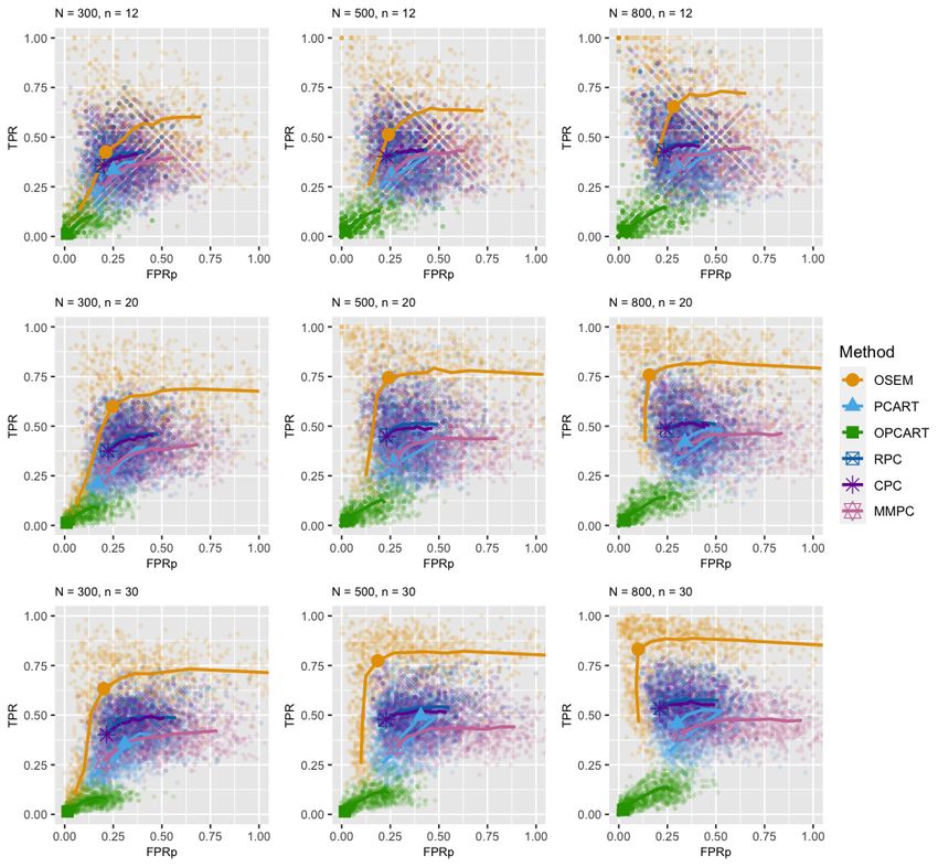
to G as
                                                              n
                                                              Y
                  p(x | θ, G) = p(x1 , . . . , xn | θ, G) =         p(xi | xpa(i) , θi , G),   (1)
                                                              i=1

where x is a realization for X, θ = ∪ni=1 θi , and the subsets {θi }ni=1 are assumed to be
disjoint. We denote the parents of node i by pa(i) such that there is an directed edge from
j to i if j ∈ pa(i). Hence, we can also read the factorization in (1) by saying that a variable
Xi is conditionally independent from its non-descendants given its parents Xpa(i) in G. This
is known as the Markov property (Lauritzen, 1996). We denote a Bayesian network by a
set B = (G, θ). Given a data sample D, learning a Bayesian network, therefore, means
estimating both the network structure G and the parameters θ.

1.1 Structure learning for Bayesian networks
Structure learning for Bayesian networks is an NP-hard problem (Chickering et al., 2004),
mainly because the number of possible DAGs grows super-exponentially with the number
of nodes n. Existing approaches to tackle this problem fall roughly into three categories:

   • Constraint-based methods perform conditional independence tests for each pair of
     nodes given a subset of adjacent nodes in order of increasing complexity. Examples
     are the PC (Spirtes et al., 2000), FCI (Spirtes, 2001), and RFCI algorithms (Colombo
     et al., 2012). These methods are fast but need to assume that the underlying graph
     is sparse (Kalisch and Bühlmann, 2007; Uhler et al., 2013).

   • Score-and-search methods rely on a scoring function and an algorithm that searches
     through the DAG space. One example is the greedy equivalence search (GES), which
     starts with an empty graph and goes through two phases of adding and removing
     edges based on the scores (Chickering, 2002). Recently, score-and-search algorithms
     based on integer linear programming have also been introduced (Cussens et al., 2017).
     More general approaches to score-and-search include sampling based methods, which
     aims to construct the full posterior distribution of DAGs given the data (Madigan
     et al., 1995; Giudici and Castelo, 2003; Friedman and Koller, 2003; Grzegorczyk and
     Husmeier, 2008; Kuipers and Moffa, 2017), as well as strategies relying on dynamic
     programming (Koivisto and Sood, 2004). These methods can be slower than the
     constraint-based ones, but in general, provide better performance when computation-
     ally feasible (Heckerman et al., 1999).

   • Lastly, the hybrid approaches bring together the above two solutions by restricting the
     initial search space using a constraint-based method in order to improve the speed and
     accuracy even further (Tsamardinos et al., 2006; Nandy et al., 2018; Kuipers et al.,
     2018).

For a broader overview on Bayesian networks we refer to the comprehensive review by Daly
et al. (2011) as well as the textbook by Koller and Friedman (2009). A recent comparison
of structure learning approaches can be found in (Constantinou et al., 2021) for example.

                                                   2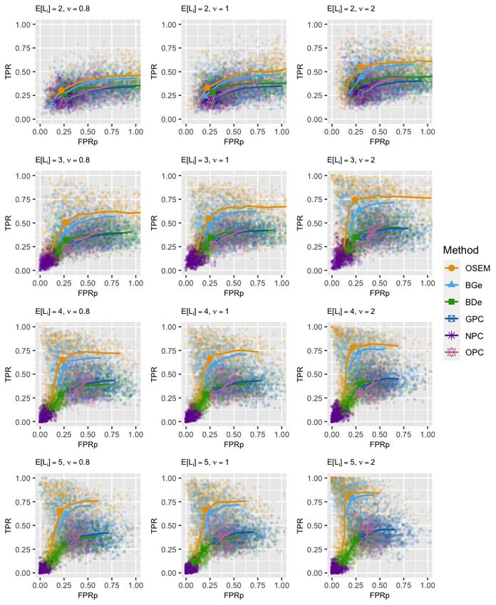
Learning Bayesian Networks from Ordinal Data

1.2 Structure learning with ordinal data
Alongside the search scheme, it is also important to properly account for the type of ran-
dom variables studied and define a suitable scoring function. The focus of this work is on
categorical variables, which can be either nominal or ordinal, depending on whether the
ordering of the levels is relevant. Examples of nominal variables include sex (male, female),
genotype (AA, Aa, aa), and fasting before a blood test (yes, no). They are invariant to any
random permutation of the categories. The listing order of the categories is, by contrast,
an inherent property for ordinal variables. Examples are stages of disease (I, II, III), survey
questions with Likert scales (strongly disagree, disagree, undecided, agree, strongly agree),
as well as discretized continuous data, such as the body mass index (underweight, normal
weight, overweight, obese), age groups (children, youth, adults, seniors) etc. (McDonald,
2009; Agresti, 2010). For discretized data, it is often difficult or impossible to access the
underlying continuous source for practical or confidential reasons. The interactions amongst
the latent variables can only manifest through their ordinal counterparts. From a techni-
cal perspective it is thus natural to think of ordinal variables as generated from a set of
continuous latent variables through discretization.
    Despite the prevalence of ordinal variables in applied research, not much attention has
been paid to the problem of learning Bayesian networks from ordinal data. One solution is
to apply constraint-based methods with a suitable conditional independence test, including
but not limited to the Jonckheere-Terpstra test in the OPC algorithm of Musella (2013),
copula-based tests (Cui et al., 2016), and likelihood-ratio tests (Tsagris et al., 2018). While a
possible extension along this line is to explore more appropriate tests to improve the search,
constraint-based methods, in general, tend to favor sparser graphs and can be dependent on
the testing order (Uhler et al., 2013; Colombo and Maathuis, 2014). In the score-and-search
regime, no scoring functions exist for ordinal variables, so metrics ignoring the ordering and
based on the multinomial distribution are the typical alternatives. An obvious drawback is
the loss of information associated with ignoring the ordering among the categories, resulting
in inaccurate statistical analyses. Another potential issue is the tendency to overparam-
eterization, especially when the number of levels is greater than 3. In this case, neither
statistical nor computational efficiency can be achieved (Talvitie et al., 2019). However, for
very large number of levels a continuous approximation may be adequate.
    In this work, we develop an iterative score-and-search scheme specifically for ordinal
data. Before describing the algorithm in detail, we briefly review the challenges. On the
one hand, we need a scoring function that can preserve the ordinality amongst the cate-
gories. On the other hand, that function should also satisfy three important properties:
decomposability, score equivalence, and consistency (Koller and Friedman, 2009). Decom-
posability of a score is the key to fast searching. Modifying a local structure does not require
recomputing the score of the entire graph, which tremendously reduces the computational
overhead. Score equivalence is less crucial but is necessary for search schemes relying on
Markov equivalent classes, such as GES or hybrid methods that initialize with a PC output.
Here, two DAGs belong to the same Markov equivalent class if and only if they share the
same skeleton and v-structures (Verma and Pearl, 1991). A Markov equivalent class can
be uniquely represented by a completed partially directed acyclic graph (CPDAG). Finally,
a consistent score can identify the true DAG if sufficient data is provided. Examples of

                                               3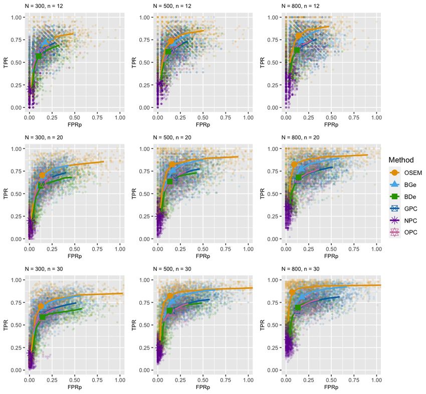
scores that satisfy all three properties are the BDe score (Heckerman and Geiger, 1995) for
(nominal) categorical data and the BGe score (Geiger and Heckerman, 2002; Kuipers et al.,
2014) for continuous data. It is, however, nontrivial to develop such a score for ordinal
data.
    To capture the ordinality, we use a widely accepted parameterization based on the
multivariate probit models (Ashford and Sowden, 1970; Bock and Gibbons, 1996; Chib and
Greenberg, 1998; Daganzo, 2014), with no additional covariates with respect to the variables
whose joint distribution we wish to model and hence focusing on their dependency structure.
As illustrated in Figure 1(a), each ordinal variable is assumed to be obtained by marginally
discretizing a latent Gaussian variable. In this case, the order of the categories is encoded
by the continuous nature of the Gaussian distribution.
    More specifically we can have at least two possible formulations, both with their pros
and cons. The first one (Figure 1(b)) assumes that the latent variables Y jointly follow
a multivariate Gaussian distribution, which factorizes according to a DAG. This approach
resembles the Gaussian DAG model (Heckerman and Geiger, 1995; Geiger and Heckerman,
2002) in the latent space, with additional connections to the ordinal variables X. Unlike in
the continuous case, marginalizing out the latent variables will result in a non-decomposable
observed likelihood. The conditional independence relationships will also disappear. This
is because DAG models are not closed under marginalization and conditioning (Richardson
et al., 2002; Silva and Ghahramani, 2009; Colombo et al., 2012). In Figure 1(b), the
Gaussian variables Y2 and Y3 are conditionally independent given Y1 , whereas the ordinal
variables X2 and X3 are not independent given X1 due to the presence of a common ancestor
Y1 in the latent space. As a result, traditional closed-form scoring functions such as the
BGe metric (Heckerman and Geiger, 1995) cannot be applied, which is generally the case
in the presence of hidden variables.
    Another setup (Figure 1(c)) uses a non-linear structural equation model with the probit
function as the link. In this case it is assumed that a DAG structure describes the relation-
ship between the observed variables, whereas the latent Gaussian variables only facilitate
the flow of information and can be marginalized out. It is equivalent to the probit directed
mixed graph model of Silva and Ghahramani (2009). In this model, the observed likelihood
is decomposable. We can recover the graph X2 ← X1 → X3 after marginalization. However,
the resulting score is not score-equivalent because the joint probability distribution fails to
meet the complete model equivalence assumption as described in (Geiger and Heckerman,
2002).
    Our solution builds on the first formulation, which we call the latent Gaussian DAG
model. The key is to observe that the complete-data likelihood is both decomposable and
score-equivalent. Further adding a BIC-type penalty will still preserve these key properties
of the score, as well as consistency (Schwarz et al., 1978; Rissanen, 1987; Barron et al.,
1998). The Structural EM algorithm of Friedman (1997) addresses the problem of struc-
ture learning in the presence of incomplete data by embedding the search for the optimal
structure into an Expectation-Maximization (EM) algorithm. We apply the Structural EM
to deal with the latent Gaussian variable construction of ordinal data in a procedure which
we call the Ordinal Structural EM (OSEM) algorithm. Note that Webb and Forster (2008)
also used the latent Gaussian DAG model and aimed to determine the network structure
from the ordinal data using a reversible jump MCMC method. Our approach differs in that

                                              4
Learning Bayesian Networks from Ordinal Data

Figure 1: (a) We assume that an ordinal variable is obtained by marginally discretizing a
          latent Gaussian variable. (b) and (c) are examples of three-node graphs for two
          different probit models discussed in Section 1.2. X1 , X2 and X3 are ordinal vari-
          ables, each obtained by discretizing a latent variable Yi with associated Gaussian
          parameters θi , i = 1, 2, 3. Latent nodes are shaded for clarity.

it explicitly exploits score decomposability, allowing for search schemes that are compu-
tationally more efficient, such as order and partition MCMC (Friedman and Koller, 2003;
Kuipers and Moffa, 2017), or hybrid methods.
    The rest of this article is structured as follows. In Section 2, we formally define the
latent Gaussian DAG model and introduce the corresponding identifiability constraints. In
Section 3, we integrate the model into the Structural EM framework. In Section 4, we
use synthetic and real data to illustrate the superior performance of our proposed method
compared to the alternatives in terms of structure recovery and prediction. In Section 5,
we apply our method to a psychological survey dataset. Finally, in Section 6, we discuss
the implications of our results as well as possible directions for future work.

2. The latent Gaussian DAG model
Let X = (X1 , · · · , Xn )> be a collection of n ordinal variables, where Xi takes values in
the set {τ (i, 1), τ (i, 2), . . . , τ (i, Li )} with τ (i, 1) < τ (i, 2) < · · · < τ (i, Li ), i = 1, . . . , n. We
assume that the number of levels Li ≥ 2, so each variable should at least be binary. It is
common to set τ (i, j) = j − 1 for all 1 ≤ j ≤ Li , i.e. τ (i, 1) = 0, τ (i, 2) = 1, and so on.
Further, we assume that each Xi is obtained by discretizing an underlying Gaussian variable
Yi using the thresholds −∞ =: α(i, 0) < α(i, 1) < · · · < α(i, Li − 1) < α(i, Li ) := ∞. Let
αi = (α(i, 0), . . . , α(i, Li ))> and α = {αi }ni=1 . The hidden variables Y = (Y1 , · · · , Yn )>
jointly follow a multivariate Gaussian distribution N (µ, Σ), which factorizes according to
some DAG G. Formally, the latent Gaussian DAG model is given by
                                                 X
          Yi | ypa(i) , ϑi , G ∼ N (µi +              bji (yj − µj ), vi )
                                             j∈pa(i)

           P (Xi = τ (i, l) | Yi = yi , αi ) = 1 yi ∈ [α(i, l − 1), α(i, l)) ,          l = 1, . . . , Li       (2)
                             Yn
           p(x, y | θ, G) =      φ(yi | ypa(i) , ϑi , G)p(xi | yi , αi )
                               i=1

                                                         5
where θ = ∪ni=1 θi with θi = (ϑi , αi ), ϑi = (µi , bi , vi ) and bi = (bji )j∈pa(i) for all i = 1, . . . , n.
Since the discretization is marginal and deterministic, the joint probability distribution
p(x, y | θ, G) remains decomposable and score-equivalent as in the Gaussian DAG model
(Geiger and Heckerman, 2002). Alternatively we can parametrize the complete joint distri-
bution of the hidden and observed variables using a mean vector µ = (µ1 , . . . , µn )> ∈ Rn
and a symmetric positive definite covariance matrix Σ ∈ Rn×n ,

                              p(x, y | θ, G) = φ(y | µ, Σ, G)p(x | y, α).                                 (3)

It follows from Silva and Ghahramani (2009) that we can write the transformation between
{bi , vi }ni=1 and Σ as
                               Σ = (I − B)−1 V(I − B)−> ,                            (4)
where (B)ij = bji and V is an n-by-n diagonal matrix with Vii = vi .

2.1 Identifiability
Different underlying Gaussian variables Y may generate the same contingency table for X,
by simply shifting and scaling the thresholds using the corresponding means and variances.
For example, we can obtain the same ordinal variable X by discretizing either Y1 ∼ N (0, 1)
at {−1, 1} or Y2 ∼ N (−1, 100) at {−11, 9}. In other words, there is not a one-to-one
mapping between the cell probabilities in the table and the parameters θ = (α, µ, Σ).
Thus, we need to impose some constraints to ensure model identifiability.
    Typically, each dimension of X requires two constraints. Webb and Forster (2008)
choose to fix the lowest and the highest thresholds for deriving the ordinal variables. For
binary variables, they restrict the only threshold at zero and set vi = 1. Instead, we find
it computationally more convenient to standardize each latent dimension. More precisely,
we let µi = 0 for all i = 1, . . . , n and constrain the covariance matrix
                                                                    √      to be in correlation
form using a diagonal matrix D := diag(d1 , . . . , dn ) with di = Σii , i.e. we replace Σ by
its transformation D−1 ΣD−1 . Due to its symmetry the correlation matrix is identified by
n(n−1)
   2    off-diagonal parameters Σij = Σji = ρij for all i 6= j. Imposing these constraints
ensures that the thresholds and the correlation matrix will be identifiable, which is sufficient
for deducing the hidden DAG G. The mean vector and the variances remain unidentifiable.

3. The Ordinal Structural EM algorithm
Given a sample DX = {x1 , . . . , xN } of size N for X, our goal is to learn both the parameters
and the structure of the Bayesian network B = (G, θ) which best explains the observed
data. Making inference about Bayesian networks with unknown structure is an intrinsically
challenging problem, and in the case of ordinal variables an additional difficulty originates
from the presence of latent variables. To estimate the parameters θ for a given DAG
G, we can use the Expectation-Maximization (EM) algorithm (Dempster et al., 1977), a
common approach to handle maximum likelihood estimation in the presence of missing
data. Conversely, with fully observed data, we may use one of the methods discussed in
Section 1.1 for structure learning. In the presence of hidden variables, the above strategies
fail, because the marginal density for X no longer decomposes over each node and its
parents. In the sequel, we consider combining the latent Gaussian DAG model with the

                                                      6
Learning Bayesian Networks from Ordinal Data

Structural EM algorithm of Friedman (1997), where the structure learning step is wrapped
inside the EM procedure. The resulting framework is the Ordinal Structural EM (OSEM)
algorithm.

3.1 The EM and the Structural EM algorithms
In the presence of latent variables, computing the maximum likelihood estimates for θ by
maximizing the observed data log-likelihood
                                               Z
                `(θ; DX ) = log p(DX | θ) = log p(DX , DY | θ)dy1 · · · dyN          (5)

can be intractable. The EM algorithm addresses this problem by alternating between two
steps:
   • E-step (Expectation): given the observed data and the current estimate of the pa-
     rameters θ(t) , t ∈ {0, 1, 2, . . . }, compute the expected value of the complete-data (in-
     cluding the hidden variables) likelihood with respect to the distribution of the hidden
     variables conditional on the observed variables,

                      Q(θ, θ(t) ) = EY|x,θ(t) [log p(DX , DY | θ)]
                                      N
                                      X                                                         (6)
                                  =         EYj |xj ,θ(t) [log p(Xj , Yj | θ) | Xj = xj ];
                                      j=1

   • M-step (Maximization): update the parameters by maximising the Q function with
     respect to θ as
                              θ(t+1) = arg max Q(θ, θ(t) ).                     (7)
                                                       θ∈Θ

The EM procedure guarantees convergence of the observed data likelihood `(θ(t) ; DX ) to a
local maximum as t → ∞ (Dempster et al., 1977).
    The Structural EM algorithm is an extension of the original EM for learning Bayesian
networks. The idea is to recursively choose a structure and a set of parameters that improve
the following expected scoring function:

           Q̃(G, θ; G (t) , θ(t) ) = EY|x,G (t) ,θ(t) [log p(DX , DY | G, θ)] −Penalty(G, θ).   (8)
                                     |                    {z                }
                                                Q(G,θ;G (t) ,θ(t) )

Here, we choose a BIC penalty term in order to ensure that the score Eq. (8) remains decom-
posable, score-equivalent, and consistent (Theorem 18.2 of Koller and Friedman (2009)). In
the following sections, we elaborate on the steps in the OSEM algorithm.

3.2 Initialization
The original algorithm of Friedman (1997) used a random initialization for both the struc-
ture G and the parameters θ. However, we can achieve faster convergence if we can cheaply
obtain rough estimates of the parameters which maximise the penalised likelihood function,
and start the EM procedure from such estimates.

                                                      7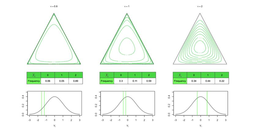
Given the identifiability constraints in Section 2.1, we only need to estimate the thresh-
olds α once at the very beginning. More precisely, given a sample DX , we can estimate the
thresholds α(i, l) for all i = 1, . . . , n and l = 1, . . . , Li − 1 as
                                                  N
                                               1 X
                              α̂(i, l) = Φ−1        1(xji ≤ τ (i, l)) ,                           (9)
                                                N
                                                   j=1

which are the empirical quantiles of the standard normal distribution.
   Next, we assume that the initial DAG G (0) is a full DAG. Conditioned on the thresholds,
we want to find the correlation matrix by maximizing the observed data log-likelihood,
                             Σ(0) | α̂ = arg max log p(DX | 0, Σ, G (0) ),                       (10)
                                             Σ
which can be computationally too expensive. Alternatively, we can use a pairwise likelihood
approach (Kuk and Nott, 2000; Renard et al., 2004; Varin and Czado, 2010), where we
estimate each off-diagonal entry ρij in the correlation matrix as
                                                    " # "        #
                  (0)                                 0    1 ρij       (0)
                 ρij | α̂ = arg max log p DXi ∪Xj |     ,           ,G       .          (11)
                               ρij                    0   ρij 1
                                            (0)
Let θ(0) = {Σ(0) , α̂} with (Σ(0) )ij = ρij for all i 6= j and (Σ(0) )ii = 1 for all i = 1, . . . , n.
This approach is fast and easy to implement at the expense of accuracy. If the resulting
correlation matrix is not positive-definite, one remedy is to smooth the matrix by coercing
the non-positive eigenvalues into slightly positive numbers. As this is only an initialization,
the difference caused by smoothing should not severely impact the following stages.

3.3 Structure update
The algorithm iterates through two steps: the structure update and the parameter update.
Given the current estimate (G (t) , θ(t) ), the structure update searches for the DAG that
maximizes the expected scoring function by computing the expected statistics instead of
the actual ones in the complete-data setting.
     In our case, computing the expected values in Eq. (6) is expensive, so we use the Monte
Carlo EM algorithm of Wei and Tanner (1990) as an approximation. For each observation
xj , we draw a sample of size K from the truncated multivariate normal distribution
                           Yj | xj , Σ(t) , α̂, G (t) ∼ TMN(0, Σ(t) | xj , α̂),                  (12)
where the sampling region of the Gaussian data is restricted to the domain specified by xj
and α̂. Then, we can approximate the expected covariance matrix as
                     N                                        N K
                   1 X                                    1 1 X X j(k) j(k) >
                       EYj |xj ,G (t) ,θ(t) (Yj )(Yj )> ≈

            Σ̂ =                                                  (y )(y ) .                     (13)
                   N                                      NK
                     j=1                                           j=1 k=1

From Eq. (2) and Eq. (3), we decompose the Q function with respect to each node and its
parents,
                        n X N                               j
                      X                                φ(Y{i}∪pa(i) | (0, Σ){i}∪pa(i) , G)
             (t) (t)
    Q(G, θ; G , θ ) =          EYj |xj ,G (t) ,θ(t) log        j
                                                                                             , (14)
                       i=1 j=1                             φ(Ypa(i)  | (0, Σ)pa(i) , G)

                                                    8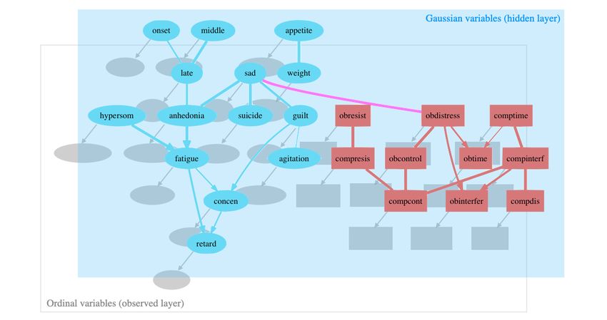
Learning Bayesian Networks from Ordinal Data

where (0, Σ)O are the parameters indexed by the set O for O ⊆ {1, . . . , n}. Let θ̂ = {Σ̂, α̂}.
By substituting Eq. (13) into Eq. (14) and using the standard normal density function, we
rewrite Eq. (8) as

                                                         log N
    Q̃(G, θ̂; G (t) , θ(t) ) = Q(G, θ̂; G (t) , θ(t) ) −         dim(G)
                                                           2
       Xn
                     N
                                                                       log N                                        (15)
                                                     −1
     =          −          log Σ̂i,i − Σ̂i,pa(i) Σ̂pa(i),pa(i) Σ̂pa(i),i −       dim(Yi , Ypa(i) ) ,
                      2                                                      2
        i=1

which is an expected version of the BIC score as in the complete-data case. Therefore, to
update the structure we need to solve the following maximization problem,

                                    G (t+1) =            arg max         Q̃(G, θ̂; G (t) , θ(t) ),                       (16)
                                                     G: DAG over (X,Y)

which we can address by using any of the existing score-based or hybrid schemes, such as
the GES and MCMC samplers.

3.4 Parameter update
Conditioned on the structure estimate G (t+1) , the goal in the parameter update is to find
θ(t+1) such that
                                                                                 log N
                   θ(t+1) = arg max Q(G (t+1) , θ; G (t) , θ(t) ) −                    dim(Yi , Ypa(i) ).                (17)
                                        θ∈Θ                                        2

The Q function can be expressed in terms of the conditional parameters from Eq. (2):
                  n X
                    N                            h                                    i
                             EYj |xj ,G (t) ,θ(t) log φ(Yij | Ypa(i)
                                                               j
                  X
                                                                     , θi , G (t+1) )
                  i=1 j=1
                  n                                          N
                                                                                                                         (18)

                            N                          1 1 X                        h                  2 i
                                                                EYj |xj ,G (t) ,θ(t) Yij − b>    j
                  X
              =         −           log(2πvi ) +                                            i Y  pa(i)       .
                            2                          vi N
                  i=1                                       j=1 |                 h   {z                  }
                                                                         PK           j(k)
                                                                                                  i
                                                                                             j(k) 2
                                                                        1
                                                                       ≈K     k=1     yi    −b>
                                                                                              i ypa(i)

The truncated multivariate normal samples in the previous structure update can be recycled
here, because the parameters θ(t) have not yet been updated. To maximize Q(G (t+1) , θ; G (t) , θ(t) )
we can then effectively use the multi-step conditional maximization (Meng and Rubin, 1993)
                                                                        (t+1)
following the topological order in G (t+1) . Suppose we have estimated θpa(i) and consider now
                            (k)               1(k)         N (k)                               (k)       1(k)    N (k)
updating θi . Let Ypa(i) = (ypa(i) , . . . , ypa(i) )> ∈ RN ×|pa(i)| and yi = (yi , . . . , yi )> ∈
RN represent the sampled design matrix and the sampled response vector respectively. We
first differentiate Q(G (t+1) , θ; G (t) , θ(t) ) with respect to bi and obtain
                                         K
                                        X                 >                K
                                                                       −1  X              >
                         (t+1)                        (k)     (k)                      (k)     (k)
                        bi          =                Ypa(i) Ypa(i)                    Ypa(i) yi              .           (19)
                                          k=1                                  k=1

                                                                   9
(t+1)
Conditioned on bi , the update for vi is then
N K
(t+1) 1 1 X X j(k) (t+1) > j(k) 2
vi = yi − (bi ) ypa(i) . (20)
NK
j=1 k=1
By introducing the BIC penalty, this procedure is equivalent to performing nodewise re-
gression with best subset selection (James et al., 2013) in the latent space. Only minor
(t+1)
modifications in the active components of bi are required.
For the purpose of identifiability and the next structure update, the final step is to
(t+1) (t+1) n
convert θ(t+1) = (bi , vi )i=1 to its corresponding correlation form with Eq. (4) and
rescaling.
3.5 Summary
The latent Gaussian DAG model assumes that the ordinal variables originate from element-
wise discretization of a set of Gaussian variables, which follow a DAG structure. Given
observations from the ordinal data only, we call Ordinal Structural EM (OSEM) algorithm
the process of estimating the hidden DAG structure, and we summarize the procedure in
Algorithm 1, along with more technical details (Supplementary Section A). Theorem 3.1 of
Friedman (1997) states that the penalized observed data log-likelihood can only improve
at each iteration, and therefore, guarantees the convergence of the algorithm to a local
optimum.
4. Experimental results
In this section, we first use simulation studies to assess the performance of our proposed
method in recovering the hidden network structure from observed ordinal data. Then, we
evaluate its predictive performance in terms of average log loss using real datasets.
4.1 Structure recovery
We randomly generate DAGs using the randDAG function from the pcalg package (Kalisch
et al., 2012), followed by generating the corresponding Gaussian data according to the
topological order in the DAGs. Then, we discretize the Gaussian data to obtain an ordinal
dataset, from which we try to learn the original structure describing the relationship between
the latent Gaussian variables. We compare our Ordinal Structural EM algorithm (OSEM)
to five other existing approaches:
1. PC algorithm with the nominal G2 test (NPC);
2. PC algorithm of Musella (2013) with the ordinal Jonckheere–Terpstra test (OPC);
3. PC algorithm with the Gaussian test using Fisher’s z–transformation (GPC);
4. hybrid method with the BDe score and NPC as initial search space (BDe);
5. hybrid method with the BGe score and GPC as initial search space (BGe).
10Learning Bayesian Networks from Ordinal Data
Note that none of these methods assume a latent Gaussian DAG model. Namely, they
all build a network model directly on the observed ordinal variables. OSEM on the other
hand estimates the hidden structure on the latent Gaussian variables. Therefore a direct
comparison of the performance with respect to the network structure needs to be taken with
caution, especially in light of the fact that conditional independence relationships do not
automatically extend from the latent to the observed space (see also Section 1.2). To the
best of our knowledge, however, no generative model for ordinal data currently exists that
provides both decomposability and score equivalence in the observed space. In the absence
of alternative methods which are capable of dealing with the latent variable construction of
ordinal data, it may still be insightful to compare the network accuracy of OSEM to that of
the most popular methods currently in use to learn network models for various data types.
Finally, to compare OSEM to other algorithms in a manner that is agnostic to the data
generating scheme, we will evaluate predictive performance on real datasets in Section 4.2.
Detailed implementations for all methods are summarised in Supplementary Section B.7.
4.1.1 Performance metrics
We assess the performance of the model by comparing the estimated structure with the
true structure. Notice that we can only identify the true DAG up to its Markov equivalence
class, so it is more appropriate to compare the corresponding CPDAGs. However, the
metrics based on CPDAG differences can still be too harsh, because many directed edges
are induced by a few number of v-structures. Therefore, we choose to compare the patterns
of the DAGs in the sense of Meek (1995), where the v-structures are the only directed edges.
In other words, we measure the structural hamming distance (SHD) between two DAGs
using the skeleton differences plus the v-structure differences.
The estimated DAG or CPDAG is first converted into a pattern. If an edge in the
estimated pattern matches exactly the same direction as the corresponding edge in the true
pattern, we count it as 1 true positive (TP). If the direction is wrong but exactly one of this
edge and the corresponding edge is undirected, then we count it as 0.5 TP. We subtract the
number of true positives from the total number of estimated edges to get the number of
false positives (FP). Furthermore, we compute the true positive rate (TPR) and the false
positive rate (FPRp) as
TP FP
TPR = and FPRp = , (21)
P P
where P is the total number of edges in the true pattern. Scaling the false positives by
P instead of the number of real negatives N can lead to a more comparable visualization,
because if the sparsity of the network stays the same, N grows quadratically as n increases.
We illustrate the comparisons mainly through Receiver Operating Characteristics (ROC)
curves. In particular, we plot the TPR against the FPRp with the following penalization
parameters:
• significance level for the conditional independence tests:
α ∈ {0.001, 0.01, 0.025, 0.05, 0.075, 0.1, 0.15, 0.2, 0.25, 0.3}.
• equivalent sample size for the BDe score:
χ ∈ {0.0001, 0.001, 0.01, 0.1, 1, 10, 20, 40, 60, 80};
11• coefficient to be multiplied by the BIC penalty:
λ ∈ {1, 1.5, 2, 2.5, 3, 4, 6, 10, 20, 30};
• coefficient to be multiplied by the precision matrix in the BGe score:
am ∈ {0.0001, 0.001, 0.01, 0.025, 0.05, 0.1, 0.25, 0.5, 1, 1.5}, and the degree of freedom
aw in the Wishart distribution is set to be n + am + 1.
Unlike comparing skeletons, the ROC curves created this way can be non-monotonic. Some
edges in the patterns may jump between being directed and undirected when the penalty
is too small or too large, so the number of TPs may not be monotonically increasing.
Furthermore, one can read the SHDs scaled by P directly from the plots, which are the
Manhattan distances from the curves to the point (0, 1).
4.1.2 Simulation results
We generate random DAGs with 4 expected neighbours per node. The edge weights are
uniformly sampled from the intervals (−1, −0.4) ∪ (0.4, 1). We consider 3 network sizes
n ∈ {12, 20, 30} and 3 sample sizes N ∈ {300, 500, 800}. For each DAG, we generate
the associated Gaussian data and perform element-wise discretization randomly using the
symmetric Dirichlet distribution Dir(Li , ν), where Li is the number of ordinal levels in the
ith dimension and ν is a concentration parameter. More specifically, we first generate the
cell probabilities in the ordinal contingency table of Xi from Dir(Li , ν). According to the
cell probabilities, we can compute reversely the thresholds for cutting the Gaussian variable
Yi using the normal quantile function (Figure S2). Here, we draw Li randomly from the
interval [2, 4] to mimic the typical number of ordinal levels and choose ν to be 2 to avoid
highly skewed contingency tables.
For each configuration, we repeat 100 times the process of randomly generating the data
and estimating the structure using the six approaches, followed by plotting the ROC curves
accordingly. Each point in Figure 2 represents a tuple (TPR, FPRp). The lines are created
by interpolating the average TPR against the average FPRp at each penalization value.
Unlike FPRn, FPRp can be greater than 1, but only points within [0, 1] are shown.
In general, the three PC-based methods alone are too conservative to recover the pat-
terns of the true underlying structures, regardless of how we increase the significance level.
Amongst them, the GPC algorithm performs the best, followed by the OPC and NPC
algorithms.
While the performance of the hybrid method with the BDe score is sometimes much
better than the PC algorithms, the upper bound of the BDe band barely touches the
lower bound of the BGe band. This observation is unanticipated in two ways. On one
hand, ignoring the ordering amongst the categories is not as harmless as one may expect.
If our modeling assumptions are correct, the common practice of using the multinomial
distribution cannot be taken for granted, as the estimated DAG can be far off. On the
other hand, the BGe score is more powerful than we may have anticipated. Even though
treating the ordinal data as continuous is inaccurate, this is still capable of detecting many
true conditional independence relationships in the latent space. Thus, leaving aside our
OSEM algorithm, one should rather use the BGe score instead of the popular BDe score
for Bayesian network learning from ordinal data.
12Learning Bayesian Networks from Ordinal Data
Figure 2: The comparison of the performance in recovering the true pattern between the
OSEM algorithm and five other existing approaches: BGe, BDe, GPC, NPC,
and OPC. The ROC curves are created by plotting the TPR against the FPRp
for sample sizes N ∈ {300, 500, 800}, network sizes n ∈ {12, 20, 30}, 3 expected
number of levels, and a Dirichlet concentration parameter of 2. Both the x-
axis and the y-axis are limited to [0, 1]. For each method, the point on the line
corresponds to the lowest SHD (the highest sum of TPR and (1 − FPRp)).
In all cases, our OSEM algorithm demonstrates a strong improvement. When the sample
size is large enough, the contingency tables are more accurate, so recovering the original
covariance structure through the EM iterations becomes more likely. With fixed sample
size, increasing the network size does not make the performance of our model deteriorate,
as long as the sparsity of the network stays the same. Additional simulation results can
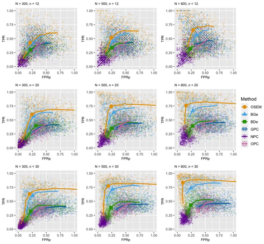
be found in Supplementary Section B, including 1) ROC curves for skeletons, 2) the effect
13of thresholds, 3) the effect of network sparsity, 4) runtimes, and 5) comparison against the
most recent structure learning methods for mixed data.
4.2 Predictive performance
For score-based approaches, we also evaluate the predictive performance using five real
ordinal datasets from McNally et al. (2017) and the UCI machine learning repository (Dua
and Graff, 2017) (Table 1). In addition to OSEM, BGe, and BDe, we have included the
PCART algorithm of Talvitie et al. (2019) for comparison, which is a score-based method
for mixed continuous, nominal and ordinal data. For each dataset and method, we train
the network with 80% of the data points, and conditioned on the structure, we compute the
log loss on the remaining 20% test cases. To ensure that the method with the continuous
BGe score has a comparable log loss, we substitute its maximum a posteriori covariance
matrix based on the estimated DAG into the OSEM log loss function, i.e. the truncated
multivariate normal density. Taking the BDe as the baseline, which is a standard choice
for categorical data, we plot in Figure 3 the relative log loss per instance corresponding
to the optimal tuning parameters over 100 random splits. We can clearly see that OSEM
consistently outperforms the baseline approach and is highly competitive across the board,
while BGe and PCART are much less robust. This further suggests that our assumption
of the ordinal data being generated from a hidden continuous space is often more valid in
practice, and the OSEM algorithm should generally be a better choice for both structure
learning and prediction. Additional details and figures can be found in Supplementary
Section B.6.
Dataset Sample size Number of variables Average levels
OCD and Depression 408 24 4.67
Congressional Voting Records 435 17 2
Contraceptive Method Choice 1473 9 3.3
Primary Tumor 339 17 2.18
SPECT Heart 267 23 2
Table 1: Description of the five real datasets in Section 4.2. Except the OCD and Depression
dataset, all other datasets are obtained from the UCI machine learning repository.
5. Application to psychological data
In this section, we provide an example applying our method to psychological survey data,
where the potential of Bayesian network models to describe complex relationships has re-
cently gained momentum (McNally et al., 2017; Moffa et al., 2017; Kuipers et al., 2019;
Bird et al., 2019). We use a dataset of size 408 from a study of the functional relationships
between the symptoms of obsessive-compulsive disorder (OCD) and depression (McNally
et al., 2017). It consists of 10 five-level ordinal variables representing the OCD symptoms
and 14 four-level ordinal variables representing the depression symptoms, measured with
the Yale-Brown Obsessive-Compulsive Scale (Y-BOCS-SR) (Steketee et al., 1996) and the
Quick Inventory of Depressive Symptomatology (QIDS-SR) (Rush et al., 2003) respectively.
14Learning Bayesian Networks from Ordinal Data
Figure 3: The relative log loss per instance with respect to the BDe baseline (dashed hor-
izontal line at 0) for OSEM, BGe, and PCART over the five datasets and 100
random splits.
Details are summarized in Supplementary Table S2. Note that “decreased vs. increased ap-
petite” and “weight loss vs. gain” in the original questionnaire QIDS-SR de facto address
the same questions from opposite directions. To avoid including two nodes in the network
representing almost identical information, we replace each pair of variables with a one seven-
level variable – appetite and weight respectively. Contradictory answers are merged into
the closest levels. For example, if “decreased appetite” receives a score of 2 and “increased
appetite” receives a score of 1, we assigns −1 to the variable appetite.
In addition to having a suitable number of observations N = 408, variables n = 24,
and an average number of levels greater than 4, we also check that none of the marginal
contingency tables have weights concentrating on one end. Thus, our OSEM algorithm is
particularly well suited in this setting. We choose the Monte Carlo sample size K to be
5 and the penalty coefficient λ to be 6, which corresponds to the highest sum of average
TPR and (1 − FPRp) on the ROC curves for N = 500, n = 20 or 30, E[Li ] = 4 or 5, and
ν = 1 from our simulations studies. The resulting CPDAG is shown in Figure 4. We depict
the nodes related to OCD symptoms with rectangles and the nodes related to depression
symptoms with ellipses. The thickness of the undirected edges reflects the percentage of
time they occur in the skeletons of 500 bootstrapped CPDAGs. If an edge is directed, then
its thickness represents its directional strength.
We reproduce the Bayesian network of McNally et al. (2017) by running the hill-climbing
algorithm with the Gaussian BIC score and retaining the edges that appear in at least 85% of
the 500 Bootstrapped networks. The corresponding CPDAG is depicted in Supplementary
Figure S10. In both graphs, the OCD and depression symptoms form separate clusters,
bridged by the symptoms of sadness and distress caused by obsessions. With the exception
of a few edge discrepancies (e.g. late – anhedonia, guilt → suicide), the two graphs appear
to be mostly similar, which is consistent with our simulation results. When the average
number of ordinal levels is relatively large, violating the hidden Gaussian assumption does
not substantially reduce the performance in recovering the true edges. Nevertheless, the
structure estimated by the OSEM algorithm should still be more reliable.
15Figure 4: CPDAG of the hidden network structure estimated via the OSEM algorithm for
the obsessive-compulsive disorder (OCD) symptoms (rectangles) and depression
symptoms (ellipses) from a dataset provided by McNally et al. (2017). The la-
belled nodes are the latent Gaussian variables, and the shaded nodes are the
corresponding observed ordinal variables. The Monte Carlo sample size K is 5,
and the penalty coefficient λ is 6. The thickness of the undirected edges reflects
the percentage of time they occur in the skeletons of 500 Bootstrapped CPDAGs.
If an edge between two labelled nodes is directed, then its thickness represents its
directional strength. For clarity, we highlight the bridge between the two clusters
of nodes (sad – obdistress).
Moreover, the CPDAG estimated using the hybrid method with the BDe score (Sup-
plementary Figure S11) is also very similar to the OSEM output, with some edges missing
and all edges undirected. The drastic difference in the simulation studies does not recur
here. A potential reason could be that the average number of parents in the true network
is fewer than one. In this case, one can check via simulations that the BDe score can some-
times provide satisfactory results without the problem of overparameterization. However,
the OSEM algorithm can handle networks that are less sparse and hence should be more
robust and preferable in practical applications. Supplementary Figure S12 is the CPDAG
estimated using the hybrid method with the BGe score. Again, since it treats the data as
continuous and uses Gaussian distribution, it looks similar to the first two networks but
slightly denser. Filtering out edges that are less certain may improve the learned structure,
but the outcome is unlikely to outperform the one from the OSEM algorithm.
Finally, we use heatmaps (Supplementary Figure S13) to visualize and compare the ad-
jacency matrices of the four CPDAGs. The shade in the grid represents the percentage of
time a directed edge appears in the 500 Bootstrapped CPDAGs, where an undirected edge
counts half for each direction. The darker the shade, the more frequent the corresponding
16Learning Bayesian Networks from Ordinal Data
directed edge occurs. There are several aspects in common: first, the symptoms of the two
questionnaires form relatively separate clusters in all four networks; second, the symptoms
appetite and weight interact with each other but are isolated from the rest of the symp-
toms; third, the connection between sad and obdistress is present in all four structures.
Nevertheless, there are also small differences between the network structures which may be
important in practice. For example, the link late – anhedonia creates a connection between
a small subset of symptoms and the largest cluster, a connection which we do not observe
in the network estimated by McNally et al. (2017). Since our simulations suggest that the
OSEM achieves better performances in structure learning from ordinal data, discovering
the connections more accurately may be highly relevant in the application domain.
6. Discussion
In this work, we addressed the problem of learning Bayesian networks from ordinal data
by combining the multinomial probit model (Daganzo, 2014) with the Structural EM algo-
rithm of Friedman (1997). The resulting framework is the Ordinal Structural EM (OSEM)
algorithm. By assuming that each ordinal variable is obtained by marginally discretizing
an underlying Gaussian variable, we can capture the ordinality amongst the categories. By
contrast, the commonly used multinomial distribution loses information related to the order
of categories due to its invariance with respect to any random permutation of the levels.
Furthermore, we assumed that the hidden variables jointly follow a DAG structure. In other
words, we have a Gaussian DAG model in the latent space, allowing us to exploit many of
its well-established properties, such as decomposability and score-equivalence.
The location and scale of the original Gaussian distribution are no longer identifiable
after discretization. Hence, we chose to standardize each latent dimension to ensure iden-
tifiability. This is computationally efficient since we only need to estimate the thresholds
once in the process.
Instead of a random initialization, we started with a full DAG and used a pairwise
likelihood approach for estimating the initial correlation matrix. This method reduces the
number of EM iterations required for convergence. We also derived closed-form formulas
for both the structure and parameter updates. In the parameter update, we can perform
regression with subset selection following the topological order of a DAG, which induces little
cost. Since our expected scoring function is decomposable, score-equivalent, and consistent,
we can perform the structure update efficiently by using existing search schemes, such as
the GES, MCMC samplers, and hybrid approaches. Unlike the reversible jump MCMC
method of Webb and Forster (2008), this additional flexibility in choosing search methods
allows us to further reduce the computational burden.
In the simulation studies, we compared the OSEM algorithm to other existing ap-
proaches, including three PC-based methods, two hybrid methods with the BDe and the
BGe scores respectively, and several methods for mixed data. Under all configurations
we tested, our method significantly improved the accuracy in recovering the hidden DAG
structure. Using real ordinal datasets, we also showed the generally superior predictive
performance of the OSEM algorithm over other score-based approaches, highlighting the
usefulness of our modelling assumptions in real applications. In addition, we demonstrated
the practicality of our method by applying it to psychological survey data.
17To our surprise, the performance of the BDe score in structure recovery was much poorer
than our method. Even though it is widely recognized that ignoring the ordering can lead to
loss of information, we are, to the best of our knowledge, the first to quantify and visualize
its impact on structural inference. The resulting deviance from the true structure was
much larger than expected. Therefore, we should in general avoid using nominal methods
to tackle problems involving ordinal data.
The BGe score, on the other hand, performed better than we had thought. The corre-
lation matrix estimated directly from the ordinal data appears to be sufficient for the BGe
score to identify many of the true edges, especially when the number of ordinal levels is
large, so that the continuous approximation improves. However, this method can hardly go
beyond the OSEM algorithm, since it still disregards the discreteness of the data.
The most dominating factor for successful structure learning is the quality of the contin-
gency tables, which is determined by the sample size, the number of levels in each ordinal
variable, as well as the position of the thresholds. First, the sample size is tightly associ-
ated with the accuracy of each cell probability, which decides to what extent the original
correlation matrix can be recovered. Second, the number and position of the thresholds
control the resolution of the contingency tables. In order to obtain a more reliable result,
it is recommended to have more than two levels for each dimension, and the weight should
not concentrate on one end of the tables. Otherwise, one may reconsider the effectiveness
of the data collected, such as whether a survey question is well-designed or whether the
target population selected is appropriate.
The PC algorithms have relatively limited accuracy in estimating the latent structures.
It could be interesting to see if a more suitable test for ordinal data can be developed,
which is in itself a challenging task. A recent method proposed by Liu et al. (2020) may
be a direction to investigate further. Furthermore, a more accurate output by the PC
algorithm can also refine the initial search space for a hybrid search scheme, such as the
method of Kuipers et al. (2018), which should in principle bring further improvements to
our OSEM algorithm.
Because of the EM iterations, the runtime of our method is unavoidably longer than
a pure score-based or hybrid approach, especially when the network size gets larger. The
main bottleneck lies in the sampling from the truncated multivariate normal distribution,
which is required in every iteration of the process. A possible direction for improvement
is a Sequential Monte Carlo sampler (Moffa and Kuipers, 2014), where the samples can be
updated from one iteration to the next instead of resampling from scratch.
Another possible direction is to create a Bayesian version of the model. One can re-
place the BIC penalty with the well-known Wishart prior (Geiger and Heckerman, 2002)
and adapt the Bayesian Structural EM algorithm of Friedman (1998). Moreover, Bayesian
model averaging (Madigan and Raftery, 1994; Friedman and Koller, 2003) may help with
the problem of reaching a local optimum. Specifically, at each iteration, one can sample
a collection of structures instead of checking only the highest-scoring graph. A sequential
Monte Carlo method can also be applied to the structure level to overcome the computa-
tional bottleneck.
Under our current model specification, it is natural to relate to the problem of Bayesian
network learning with mixed data. In particular, one may obtain a dataset with both
continuous and ordinal variables by first generating a Gaussian dataset according to a DAG
18Learning Bayesian Networks from Ordinal Data
structure and then discretizing some of the variables while keeping others continuous. A
similar learning framework may be applicable in this setting. The situation, however, can
become much more sophisticated when one wants to include nominal categorical variables.
It would therefore be interesting to extend OSEM to mixed continuous and categorical data
and compare with other existing approaches (Cui et al., 2016; Tsagris et al., 2018; Talvitie
et al., 2019).
Acknowledgements
The authors would like to thank Niko Beerenwinkel for helpful comments and discussions
and for hosting Xiang Ge Luo during her Master’s Thesis.
19References
A. Agresti. Analysis of ordinal categorical data, volume 656. John Wiley & Sons, 2010.
J. Ashford and R. Sowden. Multi-variate probit analysis. Biometrics, pages 535–546, 1970.
A. Barron, J. Rissanen, and B. Yu. The minimum description length principle in coding
and modeling. IEEE Transactions on Information Theory, 44:2743–2760, 1998.
J. C. Bird, R. Evans, F. Waite, B. S. Loe, and D. Freeman. Adolescent paranoia: prevalence,
structure, and causal mechanisms. Schizophrenia bulletin, 45:1134–1142, 2019.
R. D. Bock and R. D. Gibbons. High-dimensional multivariate probit analysis. Biometrics,
pages 1183–1194, 1996.
S. Chib and E. Greenberg. Analysis of multivariate probit models. Biometrika, 85:347–361,
1998.
D. M. Chickering. Optimal structure identification with greedy search. Journal of machine
learning research, 3:507–554, 2002.
D. M. Chickering, D. Heckerman, and C. Meek. Large-sample learning of Bayesian networks
is NP-hard. Journal of Machine Learning Research, 5:1287–1330, 2004.
D. Colombo and M. H. Maathuis. Order-independent constraint-based causal structure
learning. The Journal of Machine Learning Research, 15:3741–3782, 2014.
D. Colombo, M. H. Maathuis, M. Kalisch, and T. S. Richardson. Learning high-dimensional
directed acyclic graphs with latent and selection variables. The Annals of Statistics, pages
294–321, 2012.
A. C. Constantinou, Y. Liu, K. Chobtham, Z. Guo, and N. K. Kitson. Large-scale empirical
validation of bayesian network structure learning algorithms with noisy data. Interna-
tional Journal of Approximate Reasoning, 131:151–188, 2021.
R. Cui, P. Groot, and T. Heskes. Copula PC algorithm for causal discovery from mixed
data. In Joint European Conference on Machine Learning and Knowledge Discovery in
Databases, pages 377–392. Springer, 2016.
J. Cussens, M. Järvisalo, J. H. Korhonen, and M. Bartlett. Bayesian network structure
learning with integer programming: Polytopes, facets and complexity. Journal of Artifi-
cial Intelligence Research, 58:185–229, 2017.
C. Daganzo. Multinomial probit: the theory and its application to demand forecasting.
Elsevier, 2014.
R. Daly, Q. Shen, and S. Aitken. Learning Bayesian networks: approaches and issues. The
knowledge engineering review, 26:99–157, 2011.
A. P. Dempster, N. M. Laird, and D. B. Rubin. Maximum likelihood from incomplete data
via the EM algorithm. Journal of the Royal Statistical Society: Series B (Methodological),
39:1–22, 1977.
20Learning Bayesian Networks from Ordinal Data
D. Dua and C. Graff. UCI machine learning repository, 2017. URL http://archive.ics.
uci.edu/ml.
N. Friedman. Learning belief networks in the presence of missing values and hidden vari-
ables. In ICML, pages 125–133, 1997.
N. Friedman. The Bayesian Structural EM Algorithm. In Proceedings of the Fourteenth
Conference on Uncertainty in Artificial Intelligence, pages 129–138, 1998.
N. Friedman and D. Koller. Being Bayesian about network structure. A Bayesian approach
to structure discovery in Bayesian networks. Machine learning, 50:95–125, 2003.
D. Geiger and D. Heckerman. Parameter priors for directed acyclic graphical models and
the characterization of several probability distributions. The Annals of Statistics, 30:
1412–1440, 2002.
P. Giudici and R. Castelo. Improving Markov chain Monte Carlo model search for data
mining. Machine learning, 50:127–158, 2003.
M. Grzegorczyk and D. Husmeier. Improving the structure MCMC sampler for Bayesian
networks by introducing a new edge reversal move. Machine Learning, 71:265, 2008.
N. Harris and M. Drton. Pc algorithm for nonparanormal graphical models. Journal of
Machine Learning Research, 14, 2013.
D. Heckerman and D. Geiger. Learning Bayesian networks: a unification for discrete and
Gaussian domains. Eleventh Conference on Uncertainty in Artificial Intelligence, pages
274–285, 1995.
D. Heckerman, C. Meek, and G. Cooper. A Bayesian approach to causal discovery. Com-
putation, causation, and discovery, 19:141–166, 1999.
G. James, D. Witten, T. Hastie, and R. Tibshirani. An introduction to statistical learning,
volume 112. Springer, 2013.
M. Kalisch and P. Bühlmann. Estimating high-dimensional directed acyclic graphs with
the PC-algorithm. Journal of Machine Learning Research, 8:613–636, 2007.
M. Kalisch, M. Mächler, D. Colombo, M. H. Maathuis, and P. Bühlmann. Causal inference
using graphical models with the R package pcalg. Journal of Statistical Software, 47:
1–26, 2012.
M. Koivisto and K. Sood. Exact Bayesian structure discovery in Bayesian networks. Journal
of Machine Learning Research, 5:549–573, 2004.
D. Koller and N. Friedman. Probabilistic graphical models: principles and techniques. MIT
press, 2009.
J. Kuipers and G. Moffa. Partition MCMC for inference on acyclic digraphs. Journal of
the American Statistical Association, 112:282–299, 2017.
21You can also read